2009/69
■
Asymmetric CAPM dependence for large dimensions:
the Canonical Vine Autoregressive Model
Andréas Heinen and Alfonso Valdesogo
Center for Operations Research
and Econometrics
Voie du Roman Pays, 34
B-1348 Louvain-la-Neuve
Belgium
http://www.uclouvain.be/core
D I S C U S S I O N P A P E R
CORE DISCUSSION PAPER 2009/69
Asymmetric CAPM dependence for large dimensions: the Canonical Vine Autoregressive Model
Andréas HEINEN1 and Alfonso VALDESOGO2 November 2009
Abstract
We propose a new dynamic model for volatility and dependence in high dimensions, that allows for departures from the normal distribution, both in the marginals and in the dependence. The dependence is modeled with a dynamic canonical vine copula, which can be decomposed into a cascade of bivariate conditional copulas. Due to this decomposition, the model does not suffer from the curse of dimensionality. The canonical vine autoregressive (CAVA) captures asymmetries in the dependence structure. The model is applied to 95 S&P500 stocks. For the marginal distributions, we use non-Gaussian GARCH models, that are designed to capture skewness and kurtosis. By conditioning on the market index and on sector indexes, the dependence structure is much simplified and the model can be considered as a non-linear version of the CAPM or of a market model with sector effects. The model is shown to deliver good forecasts of Value-at-Risk.
Keywords: asymmetric dependence, high dimension, multivariate copula, multivariate GARCH, Value-at-Risk.
JEL Classification: C32, C53, G10
1Departamento de Estadistica, Universidad Carlos III de Madrid, Spain. E-mail: [email protected] 2CREA, University of Luxembourg, Luxembourg. E-mail: [email protected]
We are grateful for comments and suggestions from Kjersti Aas, Luc Bauwens, Loran Chollete, Roger Cooke, Claudia Czado, Christian Gouriéroux, Christian Hafner, Harry Joe, Dorota Kurowicka, Sébastien Laurent, Hans Manner, Andrew Patton, Michael Rockinger, Kevin Sheppard and Timo Teräsvirta, seminar participants at CORE, Exeter, Groningen, Luxembourg School of Finance, Quantitative Products Laboratory, Technical University Munich, Universidad de las Islas Baleares, Yonsei, as well as the participants of the Econometric Society European Meeting, Barcelona, August 2009, the Far Eastern and South Asian Econometric Society Meeting in Tokyo, August 2009, the Society of Financial Econometrics conference in Geneva, June 2009, the Humboldt-Copenhagen Conference, Berlin, March 2009 and the Second Vine Copula Workshop in Delft, December 2008. Andréas Heinen acknowledges support of the Spanish government grant SEJ2006-03919. Alfonso Valdesogo acknowledges financial support from the contract “Projet d’Actions de Recherche Concertées” no. 07/12-002 of the “Communauté française de Belgique”, granted by the “Académie Universitaire Louvain”. The usual disclaimers apply.
This paper presents research results of the Belgian Program on Interuniversity Poles of Attraction initiated by the Belgian State, Prime Minister's Office, Science Policy Programming. The scientific responsibility is assumed by the authors.
1
Introduction
Taking account of conditional volatilities and dependence is key for solving many financial problems, including optimal portfolios and risk management. A large literature has been devoted to univariate volatility modelling, following Engle (1982). In recent years, attention has shifted to the joint study of large cross-sections of asset returns. The first multivariate models that were proposed in the literature were the Constant Conditional Correlation (CCC) model of Bollerslev (1990), the VEC model of Bollerslev, Engle & Wooldridge (1988) and the BEKK model of Engle & Kroner (1995). For a recent survey of multivariate GARCH models, see Bauwens, Laurent & Rombouts (2006) and Silvennoinen & Tersvirta (2007). Recently, Engle (2002) introduced the Dynamic Conditional Correlation (DCC) model, which has become the benchmark for multivariate volatility models. The approach consists first in using a set of univariate GARCH models for each one of the nassets and then to model the n(n−1)/2 pairs of correlations jointly. These approaches work for moderately sized problems (up to 30 stocks in Cappiello, Engle & Sheppard (2006), who propose and estimate asymmetric DCC models for thirty stock and bond indexes). Another strand of the literature uses copulas in order to bring more flexibility to the modeling of dependence. For instance Patton (2006a) introduces bivariate models of time-varying copulas that allow for departures from normality and symmetry in the dependence, while Jondeau & Rockinger (2006) work with symmetric time-varying copulas for four stock indexes. Lee & Long (2009) use copulas to model non-linear dependence in the innovations of a DCC model for trivariate data, but they mention how to their approach could be extended to higher dimension. One remaining challenge in multivariate GARCH models is to come up with flexible distributions and models that are also feasible for the joint returns of large sets of assets. Andersen, Bollerslev, Christoffersen & Diebold (2006) study volatility and correlation models in the context of risk management and note that “the viability of [copula] methods in very high-dimensional systems remains to be established” (p. 533).
In this paper we introduce the canonical vine autoregressive (CAVA) model, a dynamic model of dependence based on canonical vine copulas, which we demonstrate to be suit-able for large cross-sections of assets (more than 30 assets) with time-varying volatilities and possibly non-Gaussian marginals. The CAVA model is not subject to size limitation, because it does not involve simultaneous estimation over the whole cross-section of assets. Our contribution is threefold. First, to the best of our knowledge, the CAVA is the only model that can be used for high dimensions, while allowing for departures from normality. Second, the model does not suffer from the curse of dimensionality, nor from an incidental parameter problem, inherent to the method of covariance targeting, used for multivariate GARCH models, see Engle, Shephard & Sheppard (2008). Moreover, there is no need to reestimate the model when more assets are taken into consideration. Third, the model can take advantage of an existing factor structure in the cross-section of stock returns in order to capture dependence in a parsimonious way. We now turn to a more detailed discussion of each of these points.
A recent literature tackles the problem of multivariate GARCH models for very large cross-sections of assets. Palandri (2009) estimates dynamic conditional correlations sequen-tially for a cross-section of 69 NASDAQ stocks. Engle & Kelly (2008), with the Dynamic
Equicorrelation (DECO) model, estimate 500 dynamic correlations under the restriction that they are equal across assets or groups of assets. Engle (2009) proposes the MacGyver estimation method which pools the autoregressive DCC parameter estimates from bivari-ate DCC models by taking their median value. Engle et al. (2008) propose an alternative estimation method for the DCC, based on selections of pairwise models, which is fast and leads to consistent estimates of the DCC parameters. While it is well-known that finan-cial returns exhibit significant departures from normality1 like leptokurtosis, skewness and asymmetric dependence,2 all these models are based on conditionally Gaussian distribu-tions. A separate literature tries to extend multivariate volatility models to non-Gaussian situations. Pesaran & Pesaran (2007) use a multivariate Student t distribution for returns, that was introduced earlier by Harvey, Ruiz & Shephard (1992). Bauwens & Laurent (2005) propose an asymmetric Student t distribution and apply it to the innovations of a DCC model for three exchange rates. Menc´ıa & Sentana (2003) use the generalized hyperbolic distribution for five NASDAQ sectorial indexes. These distributions introduce additional parameters and cannot readily be used in large dimensions. To the best of our knowledge, the CAVA model is the first one that allows realistic modelling of the empirical features of the joint distribution of returns for large cross-sections of assets. Our modeling strategy allows for a great deal of flexibility in the conditional distribution as well as the dynamics. In particular we are not restricted to Gaussian GARCH models and we can accommodate fat tails and asymmetry in the marginal distributions. Moreover time-varying canonical vine copulas allow for departures from a Gaussian dependence structure, like asymmetric dependence and tail dependence.
Most existing models of volatility and correlation suffer in one way or another from the curse of dimensionality. This means that when these models are applied to a large cross-section of assets, the number of parameters that need to be estimated jointly becomes prohibitively large, rendering estimation impossible. Another problem with multivariate GARCH models is the need to ensure that the variance covariance matrix of returns is always positive semidefinite. The DCC avoids this problem, but still suffers from the fact that ann-dimensional variance covariance matrix needs to be inverted for each observation in the evaluation of the likelihood. Moreover, models like the BEKK and the DCC must be based on targeting in order to be estimable in large dimensions (n > 30). In the case of the DCC this means that one needs an estimate of the variance covariance matrix of the standardized residuals of the univariate GARCH models and that the DCC parameters are estimated conditionally on these n(n−1)/2 parameters. Engle et al. (2008) show that, due to the incidental parameter problem, this leads to strong downward biases in estimates of the autoregressive parameters of the DCC when the numbernof assets under consideration gets very large. The CAVA model does not suffer from these problems. The basic idea underlying our model is that of conditioning. This is the building principle for canonical vine copulas. Following Sklar (1959), we decompose the joint distribution of all returns into the product of the marginals and the canonical vine copula, which captures all 1Richardson & Smith (1993) find that stock returns and their idiosyncratic risk, as measured by the residuals from the Capital Asset Pricing Model (CAPM) exhibit significant departures from normality, both in the marginal and in the dependence structure.
2For evidence on asymmetry, see Longin & Solnik (1995), Longin & Solnik (2001), Ang & Chen (2002), Ang & Bekaert (2002), Das & Uppal (2004) and Patton (2004), amongst others.
the dependence between the returns. Canonical vine copulas were developed by Bedford & Cooke (2002) and introduced into financial modelling by Aas, Czado, Frigessi & Bakken (2009). Chollete, Heinen & Valdesogo (2009) use canonical vines in a regime-switching framework and show that they are capable of capturing the asymmetric dependence that is present in international financial returns. Canonical vines are multivariate copulas obtained as a product of iteratively conditioned bivariate copulas. Therefore using as building blocks bivariate copulas, one can construct a very flexible multivariate canonical vine copula. The CAVA model consists in making each one of these bivariate copulas potentially time-varying. We propose an autoregressive model of the copula parameter that can be applied to any copula in the same way, which facilitates comparison of the time variation across copulas. This adds a lot of flexibility, as the dynamics is not constrained to be identical across pairs of assets, contrary to the DCC model. Moreover, since the model is formulated in terms of bivariate dependence models, there is no need to estimate all the parameters simultaneously. The decomposition of the joint distribution into the product of the marginals and a product of iteratively conditioned bivariate copulas opens the way for a stepwise estimation method that results in a series of low-dimensional optimizations for bivariate dynamic conditional copulas as in Patton (2006b). This means that while the estimation effort doubles if the cross-sectional dimension doubles, the complexity remains the same and the estimation just takes twice as long, since we have to carry out twice as many elementary estimations. Thus it suffers neither from the curse of dimensionality nor from the incidental parameter problem, since the estimation is stepwise and conditional; and it does not require any multivariate non-linear constraint, like positive definiteness, since it is constructed on the basis of a well-defined multivariate distribution.
Finally, the CAVA model is designed to take advantage of an existing factor structure in the cross-section of stock returns in order to capture dependence in a parsimonious way. In its full generality, a canonical vine copula amongnvariables comprisesn(n−1)/2 bivariate copulas. The CAVA model concentrates attention on the parts of the distribution which are most relevant from a financial point of view, namely the bivariate dependence models of each stock with the market. In building our model we add to the cross-section of stocks the market return and sectorial indexes. We show that once the stock returns are conditioned on the market and the sector returns, most of the dependence has been captured adequately. Our strategy consists in carefully modeling the dependence between each individual stock and the market return as well as the individual stock return and its sector return, conditioned on the market. Thus, in this version, the CAVA model can be viewed as a non-linear and non-Gaussian extension of the Capital Asset Pricing Model (CAPM) model with sectorial effects.
The paper proceeds as follows. Section 2 presents the Canonical Vine autoregressive (CAVA) model. Section 3 presents the stepwise estimation method. Section 4 deals with the model specification. Section 5 presents the empirical results for 95 weekly S&P500 stock returns as well as the results of an evaluation of VaR. Section 6 concludes.
2
The Canonical Vine Autoregressive Model
In this section, we introduce the Canonical Vine Autoregressive model (CAVA). We first provide a brief account of copula theory and canonical vine copulas, which we use to
describe the dependence. Then we show how we introduce dynamics in the model. Finally we explain how we adapt a canonical vine to obtain a very flexible factor model for the cross-section of returns, which can be viewed as a time varying and non-linear extension of the Capital Asset Pricing Model (CAPM).
2.1 Canonical Vine Copula
Traditionally in finance, the question of the dependence between returns has been addressed using Pearson’s correlation. This is due in part to the central role of the normal distribution in statistics and of the CAPM in finance. The CAPM assumes multivariate normality of returns and measures dependence with correlation. A limitation of Pearson’s correlation is that it is implicitly based on the assumption of normality, or more precisely it is only a natural measure of dependence in the elliptical family of distributions. The most prominent members of this family are the multivariate Gaussian and Student t distributions. Another limitation of Pearson correlation is that it only measures linear dependence and therefore misses non-linear relations between variables.3
In empirical finance, there is a vast body of literature suggesting that financial returns are not normally distributed. Thus, financial returns might display more intricate types of dependence than what can be captured by the correlation coefficient. One way of accounting for these more flexible types of dependence is through the use of copulas. Copulas are a very flexible tool to model patterns of dependence between variables separately from their marginal distributions, and may be used to model the observed dependence between financial returns.4 Since we are interested in modeling financial returns, in the remainder we will use a variety of GARCH models with Gaussian, Student and skewed Student t marginal distributions. These models provide the necessary flexibility to capture the main features of returns distributions like heteroscedasticity, leverage, asymmetry and leptokurtosis.
While there exist many bivariate families of copulas, the choice is much more limited for multivariate copulas. Archimedean copulas can be generalized to the multivariate case, but they imply the strong restrictions that the dependence is the same across all pairs of variables. Only the Gaussian and Student t copulas offer the possibility of having differences in the dependence between pairs of variables. Unfortunately the Gaussian copula cannot account for tail dependence, while the Student t copula restricts upper and lower tail dependence to be equal. Actual returns, on the other hand, tend to exhibit more lower than upper tail dependence, which corresponds to the idea that different stocks are more likely to crash together, than to thrive together.
We now describe the family of copulas that we use in this paper. Bedford & Cooke (2002) introduce canonical vine copulas and Aas et al. (2009) and Berg & Aas (2007), whose presentation we follow here, are the first to use them in a financial application. These very flexible multivariate copulas are obtained by a hierarchical construction. The main idea is that a flexible multivariate copula can be decomposed into a cascade of bivariate copulas. 3For instance Embrechts, McNeil & Straumann (2002) demonstrate how Pearson correlation can fail to capture dependence adequately.
4Copula theory goes back to the work of Sklar (1959). A more detailed account of copulas can be found in Joe (1997), Nelsen (1999) and in Cherubini, Luciano & Vecchiato (2004) who provide a more finance-oriented presentation. For work on copulas as a modeling tool for returns, see Embrechts, Kl¨uppelberg & Mikosch (1997), and Dias & Embrechts (2004).
It is well known that the joint probability density function ofnvariables y1, . . . , yn can be decomposed without loss of generality by iterative conditioning, as follows:
f(y1, . . . , yn) =f(y1)·f(y2|y1)·f(y3|y1, y2). . . f(yn|y1, . . . , yn−1).
Each one of the factors in this product can be decomposed further using conditional copulas. For instance the first conditional density can be decomposed as the copula function c12 linkingy1 and y2, multiplied by the density of y2:
f(y2|y1) =c12(F1(y1), F2(y2))f2(y2),
whereFi(.) denotes the cdf of yi. In the same way, one (among several) possible decompo-sition of the second conditional density is:
f(y3|y1, y2) =c23|1(F2|1(y2|y1), F3|1(y3|y1))f(y3|y1),
where c23|1 denotes the conditional copula of y2 and y3, given y1. Further decomposing
f(y3|y1) leads to:
f(y3|y1, y2) =c23|1(F2|1(y2|y1), F3|1(y3|y1))c13(F1(y1), F3(y3))f3(y3).
Finally, combining the last expressions, one obtains the joint density of the first three variables in the system as a function of marginal densities and bivariate conditional copulas:
f(y1, y2, y3) = f1(y1)f2(y2)f3(y3)·c12(F1(y1), F2(y2))·c13(F1(y1), F3(y3))·
c23|1(F2|1(y2|y1), F3|1(y3|y1)). (1) The copula density can be written as:
c(F1(y1), F2(y2), F2(y3)) =c12(F1(y1), F2(y2))c13(F1(y1), F3(y3))c23|1(F2|1(y2|y1), F3|1(y3|y1)). Conditional distribution functions are computed using a formula of Joe (1996):
F(y|v) = ∂Cy,vj|v−j(F(y|v−j), F(vj|v−j)
∂F(vj|v−j)
,
where v−j denotes the vectorv excluding the component vj. This decomposition leads to a canonical vine, in which one variable plays a pivotal role, in our example, y1. In the first stage of the copula we model the bivariate copulas ofy1 with all other variables in the system. Then we condition ony1, and consider all bivariate conditional copulas ofy2 with all other variables in the system etc. For an n-dimensional set of variables, this leads to then-dimensional canonical vine copula density:
c(F1(y1), . . . , Fn(yn)) = n−1 Y j=1 n−j Y i=1 cj,j+i|1,...,j−1(F(yj|y1, . . . , yj−1), F(yj+i|y1, . . . , yj−1)),
where the conditioning set is empty ifj= 1.
The advantages of a canonical vine copula are immediately apparent: whereas there are only very few flexible multivariate copulas, there exists a wide menu of bivariate copulas. When specifying a canonical vine copula, we can therefore choose each one of the building blocks involved from a very long list, which allows for a very large number of possible copulas. In a sense, this reverses the traditional problem of not having enough multivariate copulas to having too many to choose from!
2.2 Dynamic Dependence
In the previous section we define the canonical vine copula that we use in this paper. Combined with GARCH models for the marginal distributions of returns, a canonical vine provides a very flexible tool to model dependence. In recent years, attention of financial econometricians has turned to models of time-varying correlations. Longin & Solnik (1995) were amongst the first to document that correlations between asset returns are not constant over time. Tse (2000) develops a test for constant correlations in a multivariate GARCH model. Engle (2002) and Tse & Tsui (2002) introduce models that are designed to capture time-varying correlations. One limitation of these models is that they are restricted to the Gaussian distribution if one models a large number of returns. It is well-known that financial returns are characterized by leptokurtosis, skewness and asymmetric dependence. Some models have been suggested in the literature, that are designed to take these features into account in multivariate GARCH models. Bauwens & Laurent (2005) introduce the asymmetric Student t distribution and evaluate its performance in terms of value-at-risk (VaR) on three exchange rates, while Menc´ıa & Sentana (2003) use the generalized hyper-bolic distribution with five sectorial indexes of the NASDAQ. Unfortunately these models are often difficult to estimate and therefore not easily applied to a large cross-section of returns.
In this paper we propose to model dependence with a canonical vine copula and we let all the bivariate conditional copulas that compose the canonical vine be potentially time varying. This requires adding time variation to a number of different bivariate conditional copulas. Several approaches have been put forth in the literature for modeling dependence with time varying bivariate copulas. This line of research was started by Patton (2004), Patton (2006a), who proposes autoregressive models of the copula parameter. A non-linear function is used, that maps the real line into the domain of the parameter of the copula. In the real line the conditional copula parameter is modeled as an ARMA(1,1) of an innovation term. The fundamental question with all the dynamic copula models is the same: what should the innovation term on the right hand side of the conditional dependence parameter be? The inputs into the copula are a pair of uniform variables (u1,t, u2,t), that can be mapped into the real line with the inverse CDF of the normal distribution: ǫt= (ǫ1,t, ǫ2,t), whereǫi,t= Φ−1(ui,t). Since the original variables are uniform [0,1], ǫi,t will be univariate standard normals. Patton (2006a) uses the cross-product of past innovations computed over ten periods for the Gaussian and Student t copulas, 101 P10
i=1ǫ1,t−iǫ2,t−i, while he uses the absolute value of the difference between the uniforms for other copulas: 101 P10
i=1|u1,t−i−
u2,t−i|. Such a model has the disadvantage that the current value is a non-linear function of lagged values of conditional dependence. Moreover, the dynamics is not easily comparable across copulas. Of course in the Gaussian world, there are some well-known suggestions in the literature: the DCC of Engle (2002), the model of Tse & Tsui (2002), used by Jondeau & Rockinger (2003) for the Student t copula, and the SCC model of Palandri (2009), who applies a linear ARMA to the Fisher transforms of conditional correlation and of an exponentially smoothed version of the cross-product of past innovations.
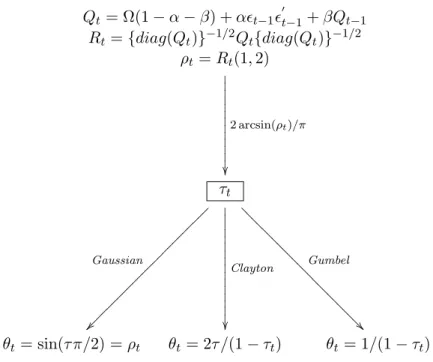
We choose, instead, to specify the time variation in the same way for all bivariate copulas, and base it on the DCC equations, as follows:
Qt= Ω(1−α−β) +αǫt−1ǫ ′
where Ω is a symmetric 2×2 matrix, with ones on the diagonal, that can be interpreted as the unconditional variance covariance matrix ofǫt, and α and β are the autoregressive parameters satisfying the restrictionsα > 0,β >0, andα+β ≤1. We standardize Qt as in the DCC:
Rt={diag(Qt)}−1/2Qt{diag(Qt)}−1/2. (3) Now ρt = Rt[1,2], the off-diagonal element of the matrix Rt, is guaranteed to be in the range [−1,1]. We then transformρtinto a Kendall’s tau:
τt= 2 arcsin(ρt)/π. (4)
The relation between the Kendall’s tau and any copula with parameterθis given by:5
τ = 4
Z
[0,1]2
C(u, v, θ)dC(u, v, θ)−1. (5)
By inverting this relation, the Kendall’s tau can be mapped into the parameter of each one of the copulas. This can be done in closed form for all the copulas we use, except for the Frank copula.6 So at each periodt, we transformτ
t, the Kendall’s tau corresponding toρt by Equation (4), into θt, the coefficient of each one of the copulas that we estimate. The specification of the dynamics is summarized in Figure 1. Equation (4) is the well-known relation between the copula parameter of the Gaussian and Kendall’s tau, see for instance Joe (1997). This implies that for every copula that we estimate, the dynamic Kendall’s tau is such thatρt can be interpreted as the parameter of the Gaussian copula that would prevail, if the copula were indeed Gaussian. The dynamic Gaussian copula obtains if we plug the parameter ρt into the density of the Gaussian copula. The same holds true for the Student t copula, except that the inverse CDF of the Student t distribution with the corresponding degrees of freedom replaces the inverse CDF of the Gaussian in the calculation ofǫt. Equations (2), (3) and (4), imply that ρt, the parameter of the Gaussian copula follows the dynamic equations of the DCC.7 Moreover, if the GARCH innovations are Gaussian and we use the Gaussian copula we recover the model of Palandri (2009), but with DCC dynamics.
There is a potential problem with the approach that we describe above. Some copulas are restricted to have positive dependence, and in that case we replace qt, the off-diagonal element ofQt by max(qt,0). This is a somewhat ad hoc way to guarantee that the model is well-defined in all situations. We do not view this as a problem, since, in general, we do not end up selecting such models. In situations where the dependence is negative during some periods, copulas that also allow for negative dependence fare much better, which translates into higher values of the likelihood. It is important to realize that the non-linear transformations fromρt to the copula parameters are part of the way in which we specify
5See for instance Embrechts et al. (2002).
6In the case of the Gumbel copula or its rotated version the transformation isθ
t = 1/(1−τt), in the
case of the Clayton, the transformation isθt= 2/(1−τt). For the Frank, the parameter obtains by solving
numerically for the solution ofτt= 1−θ4t[1−D1(θt)], whereDk(x) is the Debye function, which is defined for any positive integerkbyDk(x) =xkk
Rx 0
tk exp(t)−1dt.
Qt= Ω(1−α−β) +αǫt−1ǫ ′ t−1+βQt−1 Rt={diag(Qt)}−1/2Qt{diag(Qt)}−1/2 ρt=Rt(1,2) τt θt= sin(τ π/2) =ρt θt= 2τ /(1−τt) θt= 1/(1−τt) 2 arcsin(ρt)/π ? ? ? ? ? ? ? ? ? ? ? ? ? ? ? ? ? ? ? ? ? ? ? ? Gumbel Clayton Gaussian
Figure 1: Dynamics of the copula parameter
This figure shows how we specify the dynamics in the copula parameters. First, the inputs into the copula are a pair of uniform variables (u1,t, u2,t), that can be mapped into the real line with the inverse CDF of
the normal distribution: ǫt = (ǫ1,t, ǫ2,t), whereǫi,t = Φ−1(ui,t). For the case of the Student t copula we
use the inverse CDF of the Student t distribution with the corresponding degrees of freedom to calculate
ǫt. Then we calculate, Qt = Ω(1−α−β) +αǫt−1ǫ
′
t−1+βQt−1. We standardize Qt like in the DCC:
Rt={diag(Qt)}−1/2Qt{diag(Qt)}−1/2. Now, the off-diagonal element of the matrixRt,ρt is transformed
into a Kendall’s tau according toτt = 2 arcsin(ρt)/π. Finally, we use the fact that there is one to one
relationship between Kendall’s tau at timet,τt, and the parameters of the copula at timet, θt, given by
τt= 4R[0,1]2C(u, v, θt)dC(u, v, θt)−1, to transform the corresponding Kendall’s tau,τt into the coefficient
of each one of the copulas that we estimate,θt.
the dynamics. We carry out estimation of the parameters of the model for each copula, but for a given pair of returns, the estimated coefficients Ω, α and β, tend to be quite similar across copulas. This is not surprising and is comparable to what happens to the parameters of a GARCH estimated with different distributional assumptions.
2.3 The Dependence Structure: a Nonlinear CAPM
In the previous section we describe the canonical vine copula that we are using in this paper. In a small dimensional case, one could simply use a full canonical vine and decompose the joint distribution to the fullest level of generality. This is the strategy followed by Aas et al. (2009) in a static non Gaussian case with five series, and by Palandri (2009) in a time varying Gaussian model. This leads to estimatingn(n−1)/2 bivariate copulas for a cross section of nstocks. In the empirical application of this paper, this means we would have to estimate the parameters of (95)(94)/2 = 4465 bivariate copulas! Given the size of
the problem at hand we prefer to follow an alternative strategy and devote more modeling effort to those parts of the model that matter most.
Financial theory has devoted a lot of attention to the cross-section of asset returns, and in particular to factor models. The most prominent model in that vein is the CAPM, which implies that the cross section of returns can be explained by a single factor, the market return. This suggests that the most relevant bivariate dependence models in the cross-section of assets are between each asset and the market. The traditional CAPM assumes joint normality of individual returnsri,t, of the market return rM,t and of the idiosyncratic cross-sectionally and serially independent error termsεi,t. This implies the following linear relation:
ri,t=βirM,t+εi,t.
There has been evidence that the factor loading βi varies over time, see amongst others Ang & Chen (2007) and more recently Kristensen & Ang (2009). Therefore in the simplest version of our model, we estimate potentially time-varying bivariate copula models for the dependence between each asset and the market, and we consider that conditionally on this, the returns can be characterized by a static Gaussian copula.
Our model goes beyond a certain number of limitations of the CAPM, like non-normality and non-linear dependence, that financial economists have long been aware of. For instance Richardson & Smith (1993) show that asset returns and residuals from CAPM exhibit significant departures from normality. We explicitly allow for departures from the normal distribution, both via more general marginal distributions and in the dependence structure via the use of copulas.
In the context of CAPM, alternative measures of risk, like semivariance, which focuses on the variability of returns on the down side was proposed by Hogan & Warren (1974), and Bawa & Lindenberg (1977) propose a downside beta as a measure of risk. Ang, Chen & Xing (2006) show that stocks with high downside risk, as measured by downside beta, tend to have higher returns in a cross-section. Hong, Tu & Zhou (2007) propose a statistic, based on exceedance correlation to test for asymmetric dependence. Ang & Chen (2002) use a regime-switching model to document the existence of asymmetries in the correlation of individual stocks and portfolios with the market. Correlations conditional on positive returns are typically found to be lower than correlations conditional on negative returns. This non-linear dependence between stocks and the market return is captured in our model with asymmetric lower tail dependent copulas. In addition, whereas CAPM assumes that the idiosyncratic error terms are independent, we model the remaining dependence conditionally on the market with a Gaussian copula. In that sense our model can be viewed as an extension of the CAPM to non Gaussian GARCH marginals with non-linear possibly time-varying dependence captured by a copula.
We propose two versions of the model. The first model, which we call the market model is a non-linear equivalent of a CAPM model, where each stock return has some potentially non-linear, dynamic and asymmetric dependence with the market. In order to clarify the structure of the model, we show the joint density implied by this model in the case of four stock returns, taken from two different sectors,S1 andS2. Denote by rM, the market return,rS1
1 andrS21 the returns of assets belonging to sector 1, andr1S2 and r2S2 the returns of assets belonging to sector 2. The market model implies the following joint distribution
for the four stocks and the market returns: f(rM, r1S1, r2S1, r1S2, rS22) = f(rM)·f(rS11)·f(r2S1)·f(rS12)·f(r2S2) M arginals ·cM,rS1 1 F(rM), F(r1S1) ·cM,rS1 2 F(rM), F(rS21) ·cM,rS2 1 F(rM), F(r1S2) ·cM,rS2 2 F(rM), F(rS22) M arket ·crS1 1 ,r S1 2 ,r S2 1 ,r S2 2 |rM F(rS1 1 |rM), F(r2S1|rM), F(rS12|rM), F(r2S2|rM) . Idiosyncratic (6) where c
M,riSj is the copula between the market and the i-th stock belonging to sector j, and crS1 1 ,r S1 2 ,r S2 1 ,r S2
2 |rM is the multivariate Gaussian copula for the dependence between the
stocks conditioning on the market.
A generalization of this model consists in enriching the factor structure with sector-specific indexes. Denote by rS1 and rS2 the returns of sector 1 and sector 2 respectively. In this configuration, each stock is assumed to depend on the market and on its own sector return. Again, the dependence considered here is potentially non-linear or asymmetric and is more general than under a standard CAPM. With respect to a full canonical vine structure, we assume that conditionally on the market, the stocks are independent of sector returns other than their own. Moreover we assume that conditionally on the market, the sectorial returns are independent. This second model, which we call the market sector model implies the following decomposition of the joint density of stock, sector and market returns:
f(rM, rS1, rS2, r S1 1 , r S1 2 , r S2 1 , r S2 2 ) = f(rM)·f(rS1)·f(rS2)·f(r S1 1 )·f(rS21)·f(r1S2)·f(r2S2) M arginals ·cM,rS1(F(rM), F(rS1))·cM,rS2(F(rM), F(rS2)) ·c M,rS1 1 F(rM), F(r1S1) ·c M,rS1 2 F(rM), F(rS21) ·c M,rS2 1 F(rM), F(r1S2) ·c M,rS2 2 F(rM), F(rS22) M arket ·c S1,r1S1|rM F(rS1|rM), F(r S1 1 |rM) ·c S1,r2S1|rM F(rS1|rM), F(r S1 2 |rM) ·c S2,r1S2|rM F(rS2|rM), F(r S2 1 |rM) ·c S2,r2S2|rM F(rS1|rM), F(r S2 2 |rM) Sectors ·crS1 1 ,r S1 2 ,r S2 1 ,r S2 2 |rM,rS1,rS2 (·). Idiosyncratic (7) where cM,rSj is the copula between the market and the sector j, c
Sj,rSji |rM is the
cop-ula between sector j and stock i of the same sector conditioning on the market and
c rS1 1 ,r S1 2 ,r S2 1 ,r S2
2 |rM,rS1,rS2 is the multivariate Gaussian copula that models the dependence
between the stocks conditioning on the market and sectors.
At this point it is important to notice that the market model and the market sector model have some common parts, namely the marginals for the market and the stocks, as well as the bivariate copulas between the market and the stocks. Another possibility, that we leave for further work, is to explore the three classical Fama & French (1992) factors instead of the market sector structure.
3
Stepwise Estimation
In this section we develop the stepwise procedure that we use to estimate the market sector model. We use a 4-step procedure that is a straightforward extension of a two-step procedure that has been studied in a time series copula context by Patton (2006a), but that also underlies the estimation of the DCC model as explained in Engle & Sheppard (2001). Both cases are applications of general theorems of Newey & McFadden (1994). We assume that the marginal distribution functions and the joint distribution function are continuous and sufficiently smooth for all required derivatives to exists.
Equation (7) shows that we can decompose the joint density function into four parts, one for the marginals, one for the dependence with the market, one that reflects the dependence structure of the stocks with the own sector conditioning on the market, and finally, one for the multivariate Gaussian copula that we use to model the dependence between the stocks conditioning on the market and the sectors. This decomposition also applies to the log-likelihood function, and this is important, since it opens the way for a stepwise estimation procedure. Without loss of generality we assume that there areJ sectors and in each sector there areI stocks. We denote byrSj the return of sectorjandr
Sj
i refers to the return of the
i-th stock belonging to sector j. DefineRM ={rM,t}tT=1,RSj ={rSj,t}
T t=1,R Sj i ={r Sj i,t}Tt=1 and R = (RM, RS1, RS2,· · · , RSJ, R S1
1 ,· · · , RSIJ). The log-likelihood L(R,Ω) is obtained as a sum of the log-likelihoods of the four components:
L(R,Ω) =L1(R;α) +L2(R;α,ΘM) +L3(R;α,ΘM,ΘS) +L4(R;α,ΘM,ΘS,ΘG), L1(R, α) = PTt=1 log(f(rM,t;αM)) +PJj=1log(f(rSj,t;αSj)) +PT t=1 PJ j=1 PI i=1log(f(r Sj i,t;α Sj i )), L2(R, α,ΘM) = PTt=1 PJ j=1log(cM,rSj(F(rM,t;αM), F(rSj,t;αSj);θM,Sj)) +PT t=1 PJ j=1 PI i=1log(cM,rSj i (F(rM,t;αM), F(ri,tSj;αSij);θM,iSj )), L3(R, α,ΘM,ΘS) = PT,J,I t,j,i log(cSj,rSj i |rM(F(rSj,t|rM;αM, αSj, θM,Sj), F(r Sj i,t|rM;αM, α Sj i , θ Sj M,i);θSj,i)), L4(R;α,ΘM,ΘS,ΘG) = PTt=1log(cG|rM,rS1,···,rSJ(·;θG)), where α = (αM, αS1,· · · , αSJ, α S1
1 ,· · ·, αSIJ), are the parameters of the marginals models, ΘM = (θM,S1,· · ·, θM,SJ, θ
S1
M,1,· · · , θ SJ
M,I) are the parameters of the bivariate copulas for the dependence with the market, while ΘS = (θS1,1, θS1,2,· · ·, θSJ,I) are the parameters of the
dependence structure of the stocks with the own sector, conditioning on the market, and ΘG is the parameter of the multivariate Gaussian copula of the stocks conditional on the market and the sectors. Finally Ω = (α,ΘM,ΘS, θG), is the collection of all parameters.
The method proceeds sequentially, as follows: ˆ α = argmax α L1(R;α), ˆ ΘM = argmax Θ0 L2(R; ˆα,ΘM), ˆ ΘS = argmax ΘS L3(R; ˆα,ΘˆM,ΘS), ˆ ΘG = argmax ΘG L4(R; ˆα,ΘˆM,ΘˆS,ΘG).
At each step, estimation is carried out conditionally on the parameters estimated in ear-lier steps. The central part of the model is the dependence with the market, and those parameters are only conditioned on the marginals, like the parameters of the DCC. The most conditioning that can occur is in the last step, when estimating the Gaussian copula. This contrasts with the method of Palandri (2009), where the conditioning is done with respect to an ever increasing set of parameters, with as many steps as the dimension of the problem. His SCC model is essentially a full decomposition of the canonical vine under normality. Our method is subject to much less snowballing of estimation error, since we condition on at most three previous steps. The market model without sectors obtains by leaving out the third step in the procedure. This estimation is straightforward and can itself be further separated. When we estimate the parameters of the marginals,α, this can be done individually: ˆ αM = argmax αM L1(R;αM), ˆ αS1 = argmax αSj L1(R;αSj), forj = 1,· · · , J ˆ αSj i = argmax αSji L1(R;αSij), forj = 1,· · · , J and i= 1,· · · , I.
We then collect all the estimates into a single vector ˆα= (ˆαM,αˆS1,· · · ,αˆSJ,· · · ,αˆ
SJ
I ). The same holds when we estimate the dependence structure with the market:
ˆ θM,Sj = argmax θM,Sj L2(R; ˆα, θM,Sj), forj= 1,· · · , J ˆ θSj M,i = argmax θSjM,i
L2(R; ˆα, θM,iSj ), forj= 1,· · ·, J and i= 1,· · · , I.
We collect the estimated parameters into a vector: ˆΘM = (ˆθM,S1,θˆM,S2,· · · ,θˆ SJ
M,I). Given the previous estimates, we can estimate the parameters of the dependence of the stocks with the own sector, as follows:
ˆ
θSj,i = argmax
θSj,i
L3(R; ˆα,Θ0ˆ , θSj,i), forj= 1,· · · , J and i= 1,· · · , I.
marginals and for iteratively conditioned bivariate copulas.8 Each one of these bivariate copula estimations is easy to carry out. This brings about important advantages of the model and of its estimation procedure. First, the complexity of the model does not depend on its size, contrarily to what happens with most MGARCH models. Second, the estimation effort is linear in the number of stocks. Finally, the model does not need to be reestimated as more stocks are added.
4
Model Specification
Our framework allows for a great deal of flexibility in the specification of the model. The building blocks of the model are marginal distributions for every asset we consider and bivariate copulas for the dependence of each asset with the market in the case of the market model, and of each asset with its sector-specific return, conditionally on the market in the case of the market sector version of the model. We choose each one of these blocks from a list of possible models. Although the models that are not nested, we use the Bayesian Information Criterion (BIC) which includes a penalty term for the number of parameters and will lead us to choose more parsimonious models.9 In the remainder of this section we first list the GARCH models that we consider, followed by the bivariate copulas that we use as building blocks for the canonical vine copula. The exact specifications of the GARCH models and bivariate copulas appear in Sections 7.1 and 7.2, respectively.
4.1 GARCH Models for the Marginal Distributions
For the marginal models we follow Cappiello et al. (2006) in selecting the best GARCH model from a list of possible models using Bayesian Information Criterion. We estimate models with Gaussian innovations, but also with the Student-t, as well as the skewed Stu-dent t distribution of Hansen (1994). The volatility specifications we consider are: GARCH [Bollerslev (1986)], GJR-GARCH [Glosten, Jagannathan & Runkle (1993)], ZARCH [Za-koian (1994)], AVGARCH [Taylor (1986)], EGARCH [Nelson (1990) Nelson (1991)], APARCH [Ding, Granger & Engle (1993)] and NARCH [Higgins & Bera (1992)].
4.2 Bivariate Conditional Copulas
The conditional bivariate copulas are the building blocks we use in order to construct a large dimensional canonical vine copula. The bivariate copulas that we consider are: Gaussian, Student t, Frank, Gumbel, rotated Gumbel and Clayton. We also consider some mixture copulas: mixture of Gaussians, Gaussian and rotated Gumbel, Gaussian and Frank, Gumbel and rotated Gumbel and Frank and rotated Gumbel.
8This further reduces the number of parameters that one is conditioning on at each step. For instance, the copula parameter between the market and a stock is estimated conditionally on only the marginal of the market and of that stock.
9Possible alternatives are the Vuong (1989) likelihood ratio test or the Clarke (2007) distribution-free test for non-nested hypotheses. However these tests are designed for pairwise comparison of models, and they can lead to rejecting both models or not ejecting any. This makes them difficult to use in our context, since we are looking to order alternative models and in particular to use a procedure that always delivers an unambiguously preferred model.
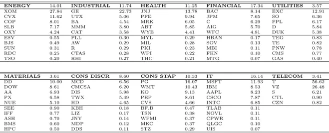
ENERGY 14.01 INDUSTRIAL 11.74 HEALTH 11.25 FINANCIAL 17.34 UTILITIES 3.57 XOM 27.84 GE 22.73 JNJ 13.78 BAC 8.14 EXC 12.91 CVX 11.62 UTX 5.06 PFE 9.94 JPM 7.65 SO 6.36 COP 8.01 BA 4.54 MRK 6.05 C 6.29 FPL 6.17 SLB 7.17 MMM 3.80 ABT 5.85 AIG 5.70 D 5.84 OXY 4.24 CAT 3.58 WYE 4.41 WFC 4.81 DUK 5.38 ESV 0.55 PLL 0.30 MYL 0.29 HBAN 0.17 TEG 0.83 BJS 0.49 AW 0.29 MIL 0.28 SOV 0.13 TE 0.82 SUN 0.31 R 0.29 PKI 0.23 MBI 0.11 PNW 0.78 RDC 0.25 CTAS 0.28 WPI 0.22 FHN 0.10 CMS 0.77 TSO 0.20 RHI 0.27 THC 0.21 MTG 0.07 GAS 0.40
MATERIALS 3.61 CONS DISCR 8.60 CONS STAP 10.33 IT 16.14 TELECOM 3.41
DD 10.00 MCD 6.56 PG 16.07 MSFT 11.93 T 56.62 DOW 8.61 CMCSA 6.20 WMT 10.43 IBM 8.53 VZ 26.48 AA 6.93 DIS 5.98 KO 9.13 AAPL 8.23 S 6.21 PX 6.58 TWX 5.49 PEP 8.61 CSCO 7.87 CTL 0.90 NUE 5.10 HD 4.65 CVS 4.66 INTC 6.85 CZN 0.82 SEE 0.90 KBH 0.18 BF.B 0.47 TLAB 0.11
IFF 0.77 LIZ 0.17 TSN 0.38 NOVL 0.11 ASH 0.70 JNY 0.14 WFMI 0.37 CPWR 0.11 BMS 0.60 MDP 0.12 MKC 0.37 QLGC 0.10 HPC 0.50 DDS 0.11 STZ 0.29 UIS 0.07
Table 1: Sample Composition and Market Capitalization shares
This table lists the S&P500 stocks that we use in the sample. The sample contains 10 stocks from each of the 10 sectorial indexes that compose the S&P500, except for the Telecom sector where only 5 stocks were present during the whole sample period. For each sector we pick the 5 largest and the 5 smallest stocks in the sector, based on market capitalization shares of June 2008.
For each of these copulas we estimate both a static and a dynamic version, except for the mixture copulas where we only consider the static case, and for each pair of returns we use the BIC to choose the best of all static and dynamic copulas.
5
Empirical Results
5.1 Data
We use a data set of returns of 95 stocks from the S&P500 downloaded from Datastream. The stocks are chosen from 10 different sectors, for which Standard and Poor reports returns. The sector indexes areEnergy, Industrials, Health, Financials, Utilities, Materials, Consumer Discretionary, Consumer Staples, Information Technology and Telecom. For each sector we pick the 5 largest and the 5 smallest stocks in terms of market capitalization data of June 2008, except for the Telecom sector, where there are only the 5 stocks that are present during all of our sample period. We use weekly data from January 1, 1995 to June 30, 2008, which gives us 703 returns. In addition to the stocks we use the S&P500 and the 10 sectorial stock indexes. Table 1 lists the tickers of the stocks we include as well as their market capitalization. For sectors the market capitalization is given as a fraction of the S&P500, while the individual stocks are quoted as a fraction of their sector.
GARCH GJR ZARCH AVGARCH EGARCH APARCH/NARCH Total
Gaussian 4 1 0 2 1 0 8
Student t 33 5 12 22 12 0 84
Skew-Student t 3 4 2 2 3 0 14
Total 40 10 14 26 16 0 106
Table 2: Summary results of the GARCH models selected by BIC criterion
This table summarizes the results of the marginal models. It breaks up the results into type of GARCH and distribution selected by the BIC criterion.
5.2 Estimation Results
As in the DCC model, the first stage of the estimation consists in selecting the best marginal model for each of the 106 return series: the S&P500 index return, the 10 sectorial index returns and the 95 stocks. A summary of the result is shown in Table 2, and the detailed result is available in the Supplemental material, in Table 10. The main difference compared to the DCC model is that we are no longer bound to the Gaussian distribution and we can allow for fatter tails with the Student t and additionally for skewness with the skewed Student t. We use a autoregressive moving average model with up to two lags for the conditional mean and select using the BIC criterion. Only 17 out of 106 series exhibit some dynamics, with AR(1) models in all cases but one, where we use an AR(2), and they are mostly sectorial index returns or big stocks. Turning to the GARCH models, we observe that the innovations are distributed as Student-t in 84 cases, where the degrees of freedom go from a minimum of 3.79 forSEE to a maximum of 12.66 for SLB. For the remaining cases the innovations are distributed as skewed Student t for 14 cases and we select a Gaussian innovation in only 8 cases.
The skewness parameters we estimate are negative in all cases except one, which implies that the distributions are negatively skewed, a well-known stylized fact of stock returns. Leaving outM SF T, the values of the skewness parameter range from−0.29 for theS&P500 index return to −0.12 for W P I. This asymmetry can be due to aggregation10 and, not surprisingly, it is found mostly in the indexes: the S&P500 and the Energy, Industrials,
Health and Financials indexes. These results show the limits of using the Gaussian as marginal distribution for the returns. Clearly, the Student t is preferred, but it does not solve all the problems, since for some of the more aggregate series, taking skewness into account is also important. As far as the dynamics of the conditional variance in concerned, we observe that the standard GARCH model is selected in 40 cases, followed by the AV-GARCH model in 26 cases. In 38% cases the selected AV-GARCH model presents some sort of leverage effect: 16 cases for the EGARCH, 14 for ZARCH and 10 for the GJR-GARCH specification. APARCH and NARCH are never selected, but some models we select are special cases of these more general specification. Given that we use the BIC criterion, that is quite conservative, this result is not surprising, as we tend to select parsimonious models. Another remarkable feature of the results is that there is clustering in the leverage effect: most of the stocks in theIndustrials andFinancials sectors present a leverage effect, while 10LetX andY be two random variables with symmetric marginals but with an asymmetric underlying copula. Then the density function ofX+Y is asymmetric.
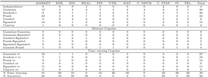
MARKET ENE. IND. HEAL. FIN. UTIL. MAT. C. DISCR C. STAP IT TEL. Total Independence 0 0 0 2 0 0 0 0 2 0 0 4 Gaussian 13 3 2 3 5 5 2 4 0 2 1 40 Student-t 6 0 1 1 3 2 1 1 3 1 1 20 Frank 22 2 3 1 0 0 3 5 1 4 1 42 Gumbel 0 0 2 2 0 0 0 0 2 0 0 6 Rgumbel 14 0 1 0 0 0 0 0 0 0 0 15 Clayton 1 0 0 0 0 0 0 0 0 0 1 2 Mixture Copulas Gaussian-Gaussian 0 0 0 0 0 0 0 0 0 0 0 0 Gaussian-Rgumbel 0 0 0 0 0 0 0 0 0 0 0 0 Gumbel-Rgumbel 0 1 0 1 0 0 0 0 0 0 0 2 Frank-Rgumbel 5 0 0 0 0 0 0 0 0 0 0 5 Rgumbel-Rgumbel 0 0 0 0 0 0 0 0 0 0 0 0 Gaussin-Frank 1 0 0 0 1 1 0 0 0 1 0 4
Time varying Copulas
Gaussian tv 18 1 1 0 0 0 3 0 2 2 0 27 Student-t tv 5 1 0 0 1 2 0 0 0 0 1 10 Frank tv 9 2 0 0 0 0 1 0 0 0 0 12 Gumbel tv 0 0 0 0 0 0 0 0 0 0 0 0 Rgumbel tv 11 0 0 0 0 0 0 0 0 0 0 11 Clayton tv 0 0 0 0 0 0 0 0 0 0 0 0 % Time Varying 41 40 10 0 10 20 40 0 20 20 20 30 % Asymetry 30 10 30 30 0 0 0 0 20 0 20 20
Table 3: Summary results of the bivariate copulas selected by BIC criterion
only two stocks in the Utilities sector have leverage, and almost none of the stocks in the
Health andUtilities sectors present a significant leverage effect.
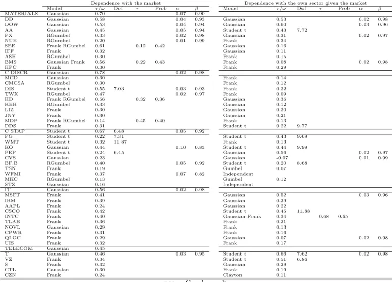
Having selected the marginal models for all series, we move to selecting all the bivariate copulas that we use as components of the canonical vine copula. Tables 3 and 4 show the results of the dependence structure of the data. The left panel of Table 4 contains the copulas for the dependence of each sector or stock with the S&P500 index return, while the right panel contains the copulas that capture the dependence between every stock and its sectorial return, conditional on the S&P500 index return. The Gaussian copula is not always selected, which is an indication that the Gaussian dependence which is underlying the traditional DCC is not appropriate. The same applies with the Student t copula. A multivariate Student t copula implies that all the dependence models with the market are Student t copulas with the same degrees of freedom for each stock or sectorial index. This is clearly not the case, again indicating that the results do not support the DCC with a multivariate Student t distribution. Moreover, in 20% of all cases the copula that we select presents some kind of asymmetry. Most of this asymmetry can be found in the dependence of stocks and sectors with the S&P500 index return. In 30% of the cases, the copulas for the dependence of the individual stocks or sectors with the market are asymmetric as can be seen in the left panel of Table 4, and the proportion is much lower in the case of sectorial dependence, conditional on the market. Not all sectors present the same kind of asymmetry in the dependence, though, and we can break up sectors into roughly three groups depending on the number of asymmetric copulas that we select for the stocks in each sector. The low asymmetry group containsFinancials (1/0)11,IT (0/0) andTelecom
(0/1), since there are almost no stocks in these sectors that present asymmetry. The second group contain sectors with low to average asymmetry. This group contains sectors where the percentage of asymmetric copulas is equal to or lower than 20%, and its members
11(x/y): x is the number of asymmetric copulas selected between the stocks of the specific sector and the S&P500 index return. y is the number of asymmetric copulas in the case of sectorial dependence, conditional on the market.
Dependence with the market Dependence with the own sector given the market
Model τ /ω Dof τ Prob α β Model τ /ω Dof τ Prob α β
ENERGY RGumbel 0.31
XOM RGumbel 0.44 0.04 0.93 Gaussian 0.63
CVX Gaussian 0.27 Gumbel RGumbel 0.54 0.61 0.50
COP Gaussian 0.24 Student t 0.80 7.40 0.02 0.97
SLB RGumbel 0.25 Frank 0.51
OXY Gaussian 0.25 Gaussian 0.44 0.03 0.97
ESV RGumbel 0.18 Gaussian 0.44
BJS Student t 0.20 7.86 Gaussian 0.42
SUN RGumbel 0.23 Frank 0.51 0.04 0.95
RDC RGumbel 0.22 Frank 0.48
TSO Clayton 0.17 Frank 0.24 0.05 0.94
INDUST RGumbel 0.86 0.05 0.93
GE Student t 0.49 6.77 Gaussian 0.61 0.04 0.91
UTX Student t 0.40 12.54 Student t 0.26 8.77
BA Gaussian 0.51 0.04 0.93 Gaussian 0.24
MMM Frank 0.34 Gumbel 0.23
CAT Frank 0.61 0.05 0.92 Gaussian 0.25
PLL RGumbel 0.44 0.05 0.91 Frank 0.11
AW Frank 0.13 0.02 0.98 RGumbel 0.05
R RGumbel 0.32 Gumbel 0.15
CTAS Student t 0.33 7.51 0.02 0.98 Frank 0.12
RHI Frank 0.59 0.05 0.91 Frank 0.07
HEALTH RGumbel 0.66 0.08 0.88
JNJ RGumbel 0.37 0.05 0.88 Gaussian 0.40
PFE Frank 0.51 0.07 0.85 Gumbel RGumbel 0.42 0.56 0.69
MRK Frank 0.52 0.07 0.87 Student t 0.42 11.56
ABT RGumbel 0.37 0.05 0.89 Gaussian 0.36
WYE Frank RGumbel 0.18 0.57 0.73 Gaussian 0.35
MYL RGumbel 0.15 Gumbel 0.09
MIL Frank 0.31 Independent
PKI Frank 0.31 Independent
WPI RGumbel 0.20 Gumbel 0.08
THC RGumbel 0.18 Frank 0.15
FINAN Student t 0.87 11.40 0.06 0.90
BAC Gaussian 0.45 Gaussian Frank 0.59 0.32 0.50
JPM Frank RGumbel 0.57 0.45 0.41 Student t 0.40 8.07
C Gaussian 0.52 Student t 0.37 13.20
AIG Student t 0.64 9.08 0.05 0.87 Gaussian 0.34
WFC Gaussian 0.42 Student t 0.39 11.11
HBAN Gaussian 0.54 0.05 0.92 Student t 0.19 8.54 0.02 0.98
SOV Gaussian 0.33 Gaussian 0.14
MBI Frank 0.57 0.06 0.88 Gaussian 0.24
FHN Frank 0.35 Gaussian 0.31
MTG Frank 0.55 0.04 0.93 Gaussian 0.24
UTIL Gaussian 0.49 0.02 0.97
EXC Gaussian 0.30 0.03 0.96 Student t 0.77 5.34 0.02 0.97
SO RGumbel 0.01 0.02 0.98 Student t 0.51 6.72
FPL Gaussian 0.34 0.03 0.96 Student t 0.71 7.69 0.04 0.86
D Gaussian 0.34 0.02 0.96 Gaussian Frank 0.59 0.35 0.68
DUK Gaussian 0.38 0.03 0.96 Gaussian 0.52
TEG RGumbel 0.21 Gaussian 0.41
Dependence with the market Dependence with the own sector given the market
Model τ /ω Dof τ Prob α β Model τ /ω Dof τ Prob α β
MATERIALS Gaussian 0.70 0.07 0.90
DD Gaussian 0.58 0.04 0.93 Gaussian 0.53 0.02 0.98
DOW Gaussian 0.53 0.04 0.94 Gaussian 0.60 0.03 0.96
AA Gaussian 0.45 0.05 0.94 Student t 0.43 7.72
PX RGumbel 0.33 0.02 0.98 Gaussian 0.31 0.02 0.97
NUE RGumbel 0.20 0.01 0.99 Frank 0.34
SEE Frank RGumbel 0.61 0.12 0.42 Gaussian 0.16
IFF Frank 0.32 Gaussian 0.11
ASH RGumbel 0.30 Frank 0.15
BMS Gaussian Frank 0.56 0.22 0.43 Frank 0.08 0.02 0.98
HPC Frank 0.30 Frank 0.29
C DISCR Gaussian 0.78 0.02 0.98
MCD Gaussian 0.30 Frank 0.14
CMCSA RGumbel 0.30 Frank 0.12
DIS Student t 0.55 7.03 0.03 0.93 Frank 0.22
TWX RGumbel 0.47 0.02 0.97 Frank 0.09
HD Frank RGumbel 0.56 0.32 0.36 Gaussian 0.36
KBH RGumbel 0.33 Gaussian 0.12
LIZ Frank 0.30 Gaussian 0.20
JNY Frank 0.30 Gaussian 0.21
MDP Frank RGumbel 0.14 0.45 0.40 Frank 0.13
DDS Frank 0.31 Student t 0.22 9.77
C STAP Student t 0.67 6.48 0.05 0.92
PG Student t 0.22 7.31 Student t 0.43 9.69
WMT Student t 0.32 11.87 Frank 0.13
KO Gaussian 0.44 0.10 0.83 Student t 0.44 9.99
PEP Student t 0.24 6.45 Gaussian 0.56 0.02 0.97
CVS Gaussian 0.23 Gaussian -0.07 0.01 0.99
BF.B RGumbel 0.40 0.05 0.92 Student t 0.20 8.68
TSN Frank 0.19 Gumbel 0.07
WFMI Frank 0.37 0.07 0.82 Independent
MKC RGumbel 0.13 Gumbel 0.12
STZ Gaussian 0.16 Independent
IT Gaussian 0.56 0.02 0.98
MSFT Frank 0.41 Gaussian 0.52 0.03 0.96
IBM Frank 0.39 Gaussian 0.29
AAPL Frank 0.24 Gaussian 0.22
CSCO Frank 0.42 Student t 0.45 11.88
INTC Frank 0.40 Gaussian Frank 0.34 0.68 0.65
TLAB Frank 0.36 Frank 0.21
NOVL Gaussian 0.29 Frank 0.13
CPWR Frank 0.31 Frank 0.16
QLGC Frank 0.29 Gaussian 0.07 0.02 0.98
UIS Frank 0.32 Frank 0.17
TELECOM Gaussian 0.45 T Gaussian 0.46 0.03 0.95 Student t 0.66 7.62 0.02 0.98 VZ Frank 0.34 Student t 0.51 6.86 S Frank 0.32 Gaussian 0.29 CTL Gaussian 0.30 Frank 0.19 CZN Frank 0.24 Clayton 0.11
Table 4:Copula results
The half left part contain the results of the dependence models of each individual stock and sector with the S&P500 market return. The half right part of the table contains the results of the
dependence between individual stock returns and the sectors given the market. ”Dof” contains the degrees of freedom for the Student t copula. ”τ /ω” refers to the Kendall’s tau in the case
Jan95 Jun99 Dec03 Jun08 0 0.1 0.2 0.3 0.4 0.5 XOM
Jan95 Jun99 Dec03 Jun08
0 0.1 0.2 0.3 0.4 0.5 PX
Figure 2: Time varying Kendall’s tau for two stocks with the market
This figure shows the time-varying Kendall’s tau implied by the estimated rotated Gumbel copulas of XOM (Energy) and PX (Materials) with the market.
areUtilities (2/0), Materials (4/0) and Consumer Staples (2/2). The last group contains sectors with more prevalent asymmetry and containsEnergy(6/1),Industrials(2/3),Health
(6/2) andConsumer Discretionary (5/0). In the case of theEnergy,Industrials andHealth
sectors, in addition to the asymmetry between the stocks and the market return, there is also asymmetry between the sectorial returns and the market. If we focus on the type of dynamics, it is striking that most of the copulas that are selected with the BIC are constant, and we select time-varying copulas only in 30% of all cases.
As far as time varying dependence is concerned, most of the selected time varying copulas are found for the dependence of stocks and sectors with theS&P500 index return. Forty-three (out of 105) of the copulas for the dependence of the individual stocks or sectors with the market are time varying. Moreover these 43 cases represent 72% of all selected time varying copulas. Another important feature is that the estimated autoregressive parameters are not equal across stocks in the same sector, nor across stocks with the same type of copula. However, there is a tendency for stocks in the same sector with time varying copula to present similar autoregressive parameters. Moreover, we find that in 13 cases the sum of the autoregressive parameters are very close to 1. This can be due to structural breaks in the dependence parameter, but plotting the time-varying dependence parameter over the sample period reveals that in most cases the dependence is smoothly trending upwards. Figure 2 plots the dynamic Kendall’s tau implied by the estimated rotated Gumbel copulas of XOM (Energy) and PX (Materials) with the market. While XOM (left panel) shows mean-reverting dependence, PX (right panel) is close to being integrated and shows an upward trend. The dynamic structure we find seems incompatible with the DCC, which implies that the autoregressive parameters are the same across all stocks.
−0.5 0 0.5 1 0
500 1000
Spearman ρ of stock returns
−0.5 0 0.5 1
0 500 1000
Spearman ρ of stock returns conditional on the market
−0.5 0 0.5 1
0 500 1000
Spearman ρ of stock returns conditional on market and sectors
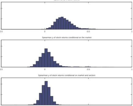
Figure 3: Histogram of Spearman rank correlation of the 95 S&P500 stock returns The three plots show the histograms of the Spearman rank correlation for all pair of assets returns. The top graph is computed on the returns after the marginal models have been estimated. The middle graph shows the Spearman correlation after the dependence with the market has been taken into account. Finally the bottom graph shows the rank correlations after the effect of the dependence with the market and the sectors have been taken out.
Figure 3 and Table 5 show how the overall level of dependence between all pairs of stocks is modified by conditioning on the S&P500 and the sectorial returns. Figure 3 shows histograms of the empirical Spearman rank correlation for all pair of assets returns. From top to bottom, it shows the Spearman rank correlation of the returns, after the marginal models have been estimated (top panel), after the dependence with the market has been taken into account (middle panel), and after the effect of the dependence with the market and the sectors have been taken out (bottom panel).12 Table 5 contains some descriptive statistics for the distributions that we plot in Figure 3. The histograms show how the Spearman rank correlations get more and more concentrated around zero after conditioning on the market (S&P500). The average Spearman rank correlation is reduced from 0.22 to 0.03, while there is no change in the standard deviation. With absolute values, the average dependence is still reduced very significantly from 0.22 to 0.07 and there is also a decrease in the standard deviation, from 0.10 to 0.08. After conditioning on the market and the sectors, the average Spearman rank correlation gets even closer to zero, from 0.03 to 0.01
12The top graph shows the empirical Spearman rank correlation of F(rS1
1 ), F(r
S1
2 ),· · ·F(r
SJ
I ), where
F(·) is the marginal model for each return. The middle graph shows the empirical Spearman rank correlation of F(rS1
1 |rM), F(r2S1|rM),· · ·, F(rSIJ|rM), where F(·|rM) is the marginal model for each
re-turn given the market. Finally the bottom graph shows the empirical Spearman rank correlation of
F(rS1 1 |rM, rS1,· · ·, rSJ), F(r S1 2 |rM, rS1,· · ·, rSJ),· · ·, F(r SJ I |rM, rS1,· · ·, rSJ), whereF(·|rM, rS1,· · ·, rSJ) is the marginal model for each return given the market and all sectors.
Mean Std dev Max Min Mean Std dev abs. value abs. value
ρS 0.22 0.10 0.81 -0.04 0.22 0.10
ρS condtional on market 0.03 0.10 0.79 -0.20 0.07 0.08
ρS cond. on market and sector 0.01 0.06 0.60 -0.35 0.04 0.04 Table 5: Descriptive statistics of Spearman rank correlation of stock returns The first line is computed with Spearman rank correlations after GARCH effects have been taken out. The second line is the same, but after the dependence with the market has also been taken out. Finally, the third line is computed after GARCH effects and dependence with market and sectors have been taken into account.
but the main change is the sharp reduction in standard deviation, from 0.10 to 0.06. The same behavior is present in the case of the absolute value of the Spearman rank correlation: the average is reduced from 0.07 to 0.04, and the standard deviation decreases from 0.08 to 0.04. These results mean that most of the dependence between stocks can be captured by theS&P500 and the sectorial returns, since, after conditioning on the market and sectors, only 33% of all possible pairs have an absolute Spearman rank correlation higher than 0.05 and this percentage is reduced to 6% when we consider an absolute Spearman rank correlation of 0.10. If the CAPM model holds, then even after controlling only linearly for the market, the idiosyncratic error terms should all be independent. However, we want to account for the fact that even though the remaining dependence is generally small, it is not exactly zero. In order to be sure that we capture the remaining dependence we estimate a multivariate Gaussian copula for the dependence between stock returns conditional on market and sector returns. A likelihood ratio test strongly rejects the null hypothesis of independence for the Gaussian copula parameter with a test statistic of 8744.2 for a 5% critical value ofχ2[95.94/2]= 4621.3, which implies a p-value of 0.00.
To summarize, our results confirm that many of the restrictions imposed on the data by the DCC can be very limiting. First, it appears clearly that the marginal distributions of the returns are not Gaussian and moreover the dependence with the market is not Gaussian, as is implied by the DCC. In 30% of the cases we select an asymmetric copula for the dependence with the market. Also, the DCC imposes that the persistence in the dependence between all pairs of assets is the same. Again our results demonstrate that this is not the case. For many assets, we find that the dependence between the market and the stocks does not vary over time. For some stocks, we find on the contrary that the sum of the autoregressive parameters is one, implying that the dynamics of the rank correlation is integrated. This shows the difficulties that arise if one restricts the dynamics to be the same for all pairs of asset, as is done in the DCC. Finally, we are able to capture nearly all the dependence present in the data, just by conditioning on the market and the sector with a dynamic and flexible copula model. For the remaining dependence we use a multivariate Gaussian copula.
5.3 Evaluation of VaR
We evaluate the performance of our model13 in terms of its ability to generate good esti-mates of Value at Risk. We use two criteria to judge performance. The first one is the likelihood ratio test of correct unconditional coverage of Kupiec (1995), based on the bi-nomial distribution. The comparison of the VaR forecast and the realized returns of the portfolio defines a sequence of binary variables, It, called hits. A hit occurs whenever the observed return is lower than the predicted VaR, resulting in a violation of the threshold. A successful VaR model at a thresholdα should have close to a fraction α of violations in sample. Kupiec (1995) proposes to testH0:f =α againstH1 :f 6=α, wheref is the fail-ure rate (estimated by ˆf, the empirical failure rate). Under the null hypothesis, the Kupiec likelihood ratio statistic LR= 2ln[ ˆfN(1−fˆ)T−N]−2ln[αN(1−α)T−N] is asymptotically distributed as aχ2(1), whereN is the number of VaR violations, T is the total number of observations (703 in our case) and α is the failure rate of the null hypothesis. The second criterion is the likelihood ratio test of conditional coverage of Christoffersen (1998). This test is a combination of the unconditional coverage and the independence tests. For the independence test, Christoffersen (1998) considers a binary first-order Markov chain for the hits, with transition probability matrix Π1
Π1 = 1−π01 π01 1−π11 π11 ,
where πi,j = P r(It = j|It−1 = i). Under the null hypothesis, H0 : π01 = π11 = α the likelihood ratio test of conditional coverage,
LR= 2ln[(1−πˆ01)n00πˆ01n01(1−πˆ11)n10πˆ11n11]−2ln[αN(1−α)T−N],
is asymptotically distributed as aχ2(2), wherenij is the number of hits with valueifollowed by j, ˆπ01=n01/(n00+n01) and ˆπ11=n11/(n10+n11).
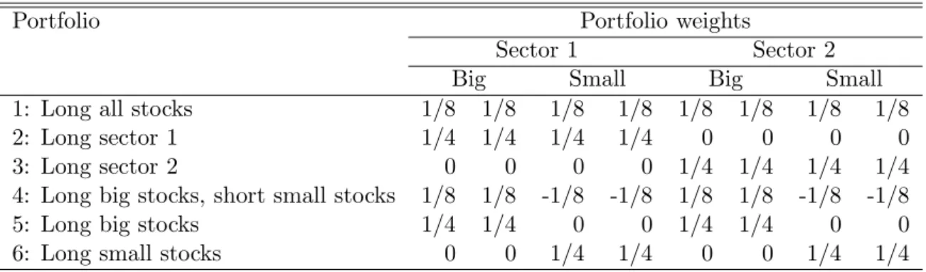
We use the DCC model as a benchmark for the evaluation of our model. The problem with the DCC in large dimensions is that it requires inversion of a large correlation matrix at each period and that its parameters suffer from a downward bias, as explained in Engle et al. (2008). Instead of attempting a direct estimation of the DCC model for the whole vector of returns, we rely on the profile likelihood approach of Engle et al. (2008) and estimate the parameters that maximize the sum of likelihoods of bivariate DCC models of 50 pairs, chosen randomly from the whole cross-section of the data. Even though our model is suitable for very large dimensional problems, we concentrate on portfolios of eight stocks, four big and four small, taken from two sectors, Health and Consumer Staples. They are, in decreasing order of market capitalization, JNJ, PFE, WPI, THC for the Health sector and PG, WMT, MKC and STZ for theConsumer Staples sector. We consider six different portfolios whose weights are shown in Table 6. We compute the upper and lower tail percentiles of these portfolios, which corresponds to analyzing the risk of, respectively, long and short positions in the portfolios of Table 6. All models are tested with a VaR14 level 13We consider only the market sector model, based on the structure of Equation (7) which, for the rest of this section we refer to as the CAVA model.
14The VaR for the CAVA model has been calculated by simulating 50.000 observations, following the algorithm of Section 7.4.
Portfolio Portfolio weights
Sector 1 Sector 2
Big Small Big Small
1: Long all stocks 1/8 1/8 1/8 1/8 1/8 1/8 1/8 1/8
2: Long sector 1 1/4 1/4 1/4 1/4 0 0 0 0
3: Long sector 2 0 0 0 0 1/4 1/4 1/4 1/4
4: Long big stocks, short small stocks 1/8 1/8 -1/8 -1/8 1/8 1/8 -1/8 -1/8
5: Long big stocks 1/4 1/4 0 0 1/4 1/4 0 0
6: Long small stocks 0 0 1/4 1/4 0 0 1/4 1/4
Table 6: Portfolios for Value at Risk computation This table shows the weights of the 6 portfolios we use to evaluate Value at Risk.
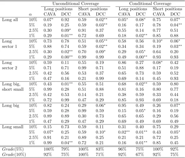
α of 10%, 5%, 2.5% and 1%, and their performance is assessed by likelihood ratio tests of correct unconditional and conditional coverage, shown in Table 7.
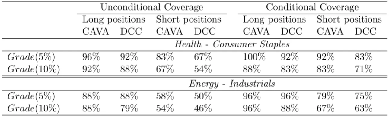
To compare the results of the models, we use a summary performance measure, Grade(β), which is the percentage of p-values above theβ critical value for long and short positions. The level of the testβ should not be confused with the level α at which VaR is evaluated. For instance, for the correct unconditional coverage test, in Table 7, when we consider long positions at the critical value β = 5%, we have 5 rejections out of 24 portfolios for the DCC, which implies that itsGrade(5%) is 79%, compared to 100% for the CAVA model. If instead we consider a critical value ofβ= 10%, we have 6 rejections for the DCC and 1 for the CAVA model, which impliesGrade(10%) of 75% for the DCC and 92% for the CAVA. Overall the CAVA model performs better than the DCC model for both the conditional and the unconditional coverage tests. We repeat this analysis with another set of stocks: XOM, OXY, ESV, TSO for the Energy sector and GE, CAT, PLL and RHI for the Industrials
sector, given in decreasing order of market capitalization. We consider the same portfolios as in the previous exercise and a summary of the results is shown in Table 8. Overall the results in terms of Grade(5%) and Grade(10%) are quite similar to the ones in Table 7. The CAVA performs better than the DCC and the main differences are in short trading positions.
So far we have evaluated VaR in-sample and this exercise can be viewed as providing diagnostics for the model. Given that the CAVA is more heavily parameterized than the DCC, it is of interest to check that its good in-sample performance carries over to an out-of-sample setting. In order to do this, we split the sample into an estimation period of 500 observations and leave 203 observations for the out-of-sample evaluation. We specify and estimate the models15 on the first 500 observations and perform a series of 203 one-step ahead VaR forecasts. Keeping the structure constant, we reestimate the parameters of each 15This includes the type of GARCH models for both the DCC and the CAVA, as well as the bivariate copulas for the CAVA model.