Computer-based simulation and validation of robot accuracy improvement method and its verification in robot calibration procedure

(1)

See discussions, stats, and author profiles for this publication at: https://www.researchgate.net/publication/334291477

Computer-based simulation and validation of robot accuracy improvement

method and its veriﬁcation in robot calibration procedure

Conference Paper · July 2019 CITATIONS

0

READS

44

6 authors, including:

Some of the authors of this publication are also working on these related projects:

Computer Aided (Filament Winding) Tape Placement for Elbows. Practically Orientated Algorithm View project

Parametric robot calibration View project Igor Dimovski

Institute for Advanced Composites and Robotics 15PUBLICATIONS 6CITATIONS

SEE PROFILE

Mirjana Trompeska

SEE PROFILE

Filip Kochoski

SEE PROFILE

Vladimir Dukovski

Ss. Cyril and Methodius University 34PUBLICATIONS 58CITATIONS

SEE PROFILE

All content following this page was uploaded by Igor Dimovski on 08 July 2019.

(2)

Computer-based simulation and validation of

robot accuracy improvement method and its

verification in robot calibration procedure

Samoil Samak, Igor Dimovski, Mirjana Trompeska,

Martin Hristoski, Filip Kochoski

Institute for Advanced Composites and Robotics Prilep, Macedonia

[email protected],[email protected],

[email protected]

Vladimir Dukovski

Faculty of Mechanical Engineering Ss. Cyril and Methodius University

Skopje, Macedonia [email protected]

Abstract—Algorithm for improving accuracy of six-axes robot

is developed and validation method based on computer simulation is implemented. Optimization is used to minimize the distances between nominal and actual positions of the tool. That way, the parameters of the robot are calibrated and using such calibrated parameters, accuracy of the robot is significantly enhanced.

Measurement is done using API Radian laser tracker and experimental data is collected on KUKA 480 R3330. For the set of 75 points used for calibration, simulation predicted reduction of the mean of the total displacement error from 1.619 mm to 0.174 mm. After that, the same points were used for verification procedure. Another measurement is performed, using the calibrated parameters and numerically calculated compensation of the machine coordinates of the robot. The mean of total displacement error was 0.293 mm and that way the correctness of described method is verified.

Keywords—robot calibration, robot accuracy, robot precision, parametric calibration, optimization

I. INTRODUCTION

The latest implementations of an industrial robots in aerospace industry, automobile industry, medicine etc, require a robot with high accuracy and repeatability. The issues related to the robot’s repeatability are less interesting for the researchers, because mostly all industrial robots satisfied the declared repeatability by the manufacturer, which is satisfactory value for the mentioned implementations. However, the declared value for robot’s accuracy isn’t satisfactory for the mentioned robot’s implementations and many researchers tend to improve the robot’s accuracy.

Robot accuracy can be affected by errors which can be categorized as geometric and geometric. The term non-geometric errors is a common name for the dynamic errors like internal loading, structural resonance, joint and link deflections caused by gravity and payload, thermal errors caused by the

expansive property of the materials and system errors like joint friction and backlash. Xi in [1] reviews the effect of the non-geometric errors on the manipulator internal calibration. During the past years there have been developed few techniques for identification and calibration of non-geometrical errors, and almost all of them identified and compensate the non-geometric errors together with the geometric errors. Zhou and Kang developed an algorithm for simultaneously identification of geometric errors and joint compliance of industrial robot based on least-square genetic algorithm [2]. Also, Tao et al. [3] using the product of exponential developed a method for calibration of the geometric errors of the robot that take into account the joint compliance. Jang et al. [4] besides the geometrical errors also identified joint compliance and gear transmission errors as non-geometric parameters of the developed model. Kamali, et al. identify joint stiffness and geometric errors using laser tracker for measuring several positions of the robots’ end-effector when the robot is subjected under wide range of external forces and torques [5]. Renders et al. [6] in their model for identification and calibration of the non-geometrical errors based on neural networks, assumed that the geometrical errors are already identified and compensated, so the residual error only contain the non-geometrical effects.

Geometric errors can cause deviations in the commanded position and orientation of the robot’s tool and are present due to imprecise manufacturing of the manipulator links and joints. Geometric errors is a common name for position dependent geometric errors (PDGE) like translational errors and rotational errors and position independent geometric (PIGE) errors like orthogonality errors and parallelism errors. More details about the PDGE and PIGE can be found in [7].

Most of the developed techniques for robot calibration identify and calibrate the geometric errors and the calibration method is based on adaptive kinematics procedure. The nominal values of the robot’s links and joints or the nominal parameters of the robot defined by the manufacturer are taken

(3)

into account in the kinematic equations. Because of the geometrical errors the actual values of the robot’s links and joints differ from the nominal parameters. The kinematic which include the actual values of the robot’s links and joints or the actual parameters is adaptive kinematics.

In order to identify the actual parameters of the robot there have been developed many techniques which basically differ in the measuring method and calibration model. The calibration procedure consists of modeling, measurement, parameter identification and compensation, [8]. Measurement techniques can be categorized as techniques with relative measuring method and absolute measuring method. The first ones identify the actual values of the robot’s links and joints by comparing the measured value with some previously known value, or by comparing two consecutive measured values. Lu and Hayes in [9] propose a relative measurement method for identification of the actual parameters by comparing two sequential images of end-effector pose obtained with camera mounted on the robot. English et al. proposed relative measurement technique where the only required measurements are the differences between the position of rulings in adjacent images and the differences in height above the flat standard [10]. In their measurement system, while the robot is moving linearly, camera mounted on a robot captures an image of a thermal-dimensionally stable ruled standard and a laser distance sensor determine the height above parallel flat standard.

Measurement techniques with absolute measuring method determine the measured value like position and/or orientation of the robot’s end-effector in absolute measuring unity. Švaco et al. determined the errors on the absolute positioning of the robot’s end-effector using a stereo vision system composed of two CCD cameras [11]. In their system the measured points are represented as spheres which are projected into circles in two different planes and captured by the cameras. The spatial coordinates of the centers of the circles are used to identify the actual position of robot’s end-effector. Joubair and Bonev used a high precision probe attached on the robot’s end-effector that touch about sixty times three equidistant spheres placed on artefact for three different orientations of the artefact [12]. The distance between each sphere is precisely determined on Coordinate Measuring Machine (CMM). The collected data are then fitted in order to obtain the actual parameters of the robot. Lui et al. determined the actual robot pose using a multiple-sensor measuring system composed of visual multiple-sensor that measures the position and angle sensor that measures the orientation of the manipulator [13]. Kihlman et al. determine the actual pose of the robot’s end-effector using a metrology system composed of laser tracker that measures a distance to a prism and camera that trough a photogrammetry measures the orientation of camera reflector [14]. The laser prism and camera reflector form a 6D reflector mounted on the robot’s end-effector. Nguyen et al. also determine the actual robot pose only with laser tracker by measuring discrete points on circular trajectory [15]. Santolaria et al. determined the actual parameters of the robot using a screw theory as a kinematic model and only laser tracker as a measuring device [16].

This paper presents an algorithm for improving accuracy of a six-axis robot KUKA 480 R3330. Screw theory is used as a mathematical model for the kinematics of the robot and

optimization method is used for calibration procedure of the robot. API Radian laser tracker is used as a measuring device in the measuring procedure where 75 points are measured for the calibration phase in order to identify the actual or calibrated parameters of the robot and 73 points are measured for the validation phase in order to estimate the correctness of the algorithm. In order to verify the estimated correctness of the proposed algorithm the same 75 points used in calibration phase are measured again, after the determination of the calibrated robot’ parameters in the verification phase.

The rest of the paper is organized as follows. Section II describes the mathematical model of the calibration procedure and kinematics of the robot based on the screw theory. In this section is also given a description of the calibration system composed of robot and laser tracker, the nominal parameters of KUKA 480 R3330 robot and the transformation needed to calculate the actual position of the robot’s tool with respect to absolute coordinate system, instead with respect to measurement frame. In section III are given details about the calibration phase of the calibration procedure i.e. determination of the robot accuracy and calibrated parameters of the robot. Section IV gives a description of the computer simulation used to estimate the correctness of the calibration algorithm and in section V are given the results obtained after the verification phase is done. The final section is reserved for the conclusions.

II. MATHEMATICAL MODEL–MINIMIZING THE TOTAL DISPLACEMENT ERROR

For N chosen points in the robot’s workspace, only the position of the tool is considered. If nominal position of ith point has coordinates with respect to Absolute Coordinate System (ACS):

Pi,nom= [Xi,nom,Yi,nom,Zi,nom]T  and respectively, the actual position is measured to be:

Pi,act= [Xi,act,Yi,act,Zi,act]T  Expressed with respect to ACS, so the ith estimated error is:

Ei=Pi,actPi,nom 

The nominal position (1) is determined by joint coordinates, but as well depends on the robot parameters. Optimization technique is applied according to parameters vectorV. The aim is to minimize the Total Displacement Error (TDE), hence the objective function is defined as:

 





 n_i norm

f(V) ₁ Ei 

A. Calibration procedure

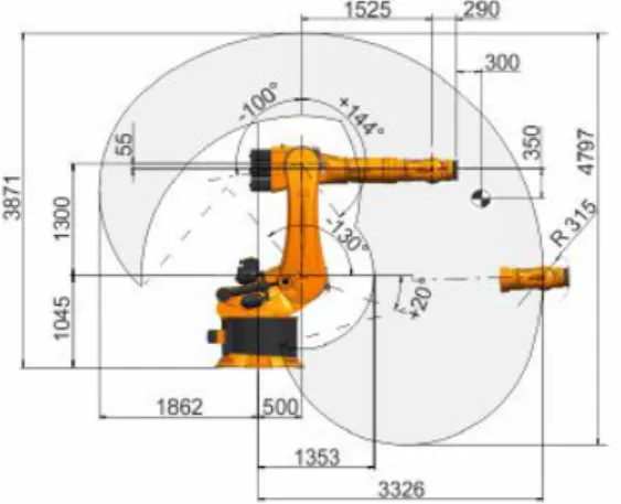
Calibration procedure is applied to 6 Degrees of Freedom (DOF) robot of type KUKA 480 R3330 (Fig. 1). This industrial robot has all 6 rotational axes. The joints of the robot are expressed in Machine Space (MC) with theta-vector of machine coordinates:

(4)





1,



2,



3,



4,



5,



6,





θ 

Developed kinematic model is used for forward kinematics transformation from Tool Frame (TF) to Base Frame (BF), based on screw theory:

 

6 6

 

0 ^ 5 5 ^ 4 4 ^ 3 3 ^ 2 2 ^ 1 1 ^ bt bt e e e e e e g g θ              

The equation (6) allows to calculate the coordinates in Pose Space (PS) if machine coordinates are known. Only last column of the matrix, as position portion of the pose is used in the calibration procedure. This procedure is used in ideal case, using the nominal robot parameters, and after calculation of the calibrated robot parameters, the same forward kinematics procedure is used in the numerical algorithm for inverse kinematics procedure for calculating the compensated coordinates in MS.

Details for forward kinematics transformation, and as well the inverse kinematics procedure could be found in [17].

In total, Nc = 75 points are randomly chosen in MS – machine coordinates are randomly generating, checking the tool positions to be distributed in entire robot’s workspace. These 75 points are used for the calibration procedure, in order to calculate the calibrated robot parameters. Also, anotherNv= 73 points in MS are randomly chosen for the validation procedure, explained in details in the section 4. Using equation (6), positions with respect to ACS are calculated as nominal positions for all, in total 148 points.

Fig. 1. Industrial robot KUKA 480 R3330

B. Nominal robot’s parameters

There are in total 36 robot’s parameters used in this mathematical model. First 24 parameters are described in sense of usually used Denavit-Hartenberg (DH) convention [18], 4 parameters for each of 6 joints. Since screw theory approach is used in the kinematic model, only 2 references are used – BF and TF. Additionally, six parameters for each reference is used, in total 12 for the references.

The column B in the Table 1 determines relative position and orientation of the BF with respect to ACS. For simplicity, as screw theory approach allows, nominally the BF is taken to

coincide with ACS. After the calibration, corrections of position (B1, B2, B3, expressed in millimeters) and corrections

of orientation as Euler angles (B4, B5, B6, expressed in degrees)

will describe calibrated relative position and orientation of the BF with respect to ACS.

TABLE I. NOMINAL PARAMETERS OF THE ROBOT

i αi(deg) di(mm) ai(mm) ϕi(deg) B T 1 0 1045 0 0 0 0 2 -90 0 500 0 0 0 3 0 0 1300 -90 0 0 4 -90 1525 -55 0 0 0 5 90 0 0 0 0 0 6 -90 290 0 180 0 0

Initially, the TF is set with respect to the robot’s flange as vector:

T0= [42.4163, -70.9065, 239.5558, -0.038, 0.237, 0.054]T 

First 3 coordinates of T0 describes the position in

millimeters of TF with respect to flange. Last 3 coordinates of

T0 describes the orientation as Euler angles in degrees, with

respect to flange.

The last column of the Table 1 contains the corrections needed to be made to the position and orientation of the TF with respect to the flange. Initially, all of them are zeros, so after the calibration these 6 parameters will describe the tool corrections.

C. Transformation from measurement frame to base frame There is one more frame that has to be taken into account. Namely, the raw data collected during the measurement are expressed with respect to Measurement Frame (MF). To transform the measured positions with respect to ACS, transformation matrix is determined using optimization technic similar to the one described in the section A.

For all measured points, the nominal position is calculated using forward kinematic procedure with nominal robot’s parameters (equation (1), for i=1,2,…, 148). The unknown transformation matrixTrcontains 12 unknown parameters t1–

t12.            1 0 0 03 6 9 12 11 8 5 2 10 7 4 1 t t t t t t t tt t t t Tr 

If measured positions with respect to MF are collected and stored as:

Mi= [Xi,m,Yi,m,Zi,m]T 

then the ith estimated error is:

(5)

The objective function is taken to be:

 





n_

 

i norm f 1 Ei,m Tr 

Initially, transformation matrix Tr is set measuring 3 points on the plane parallel to the base plane of the robot.

III. CALIBRATION PHASE

A. Measurement before calibration - results

The measurement is performed using Laser Tracker – interferometer produced by company API (Automated precision). The data is collected for 151 positions – 75 points for calibration phase, 73 points for validation phase and 3 points for determination of the initial values of transformation matrixTr.

Once the matrixTris determined, estimated errors for the set of 75 points for the calibration phase is calculated using (3), as a norm of the displacement error. The vector of estimated errors for the set of 73 points for the validation process are calculated as well. The mean, standard deviation and maximum of these estimated errors for both sets of points are shown in Table 2.

TABLE II. MEASURED ERROR BEFORE CALIBRATION

Calibration phase

points Validation phasepoints

Mean (mm) 1.619 1.603

St. dev. 0.269 0.272

Max. (mm) 2.268 2.173

B. Calibrated robot’s parameters

Optimization procedure described in section 2 is performed to determine the calibrated robot’s parameters in order to minimize the objective function (4).

For the calibration phase, only the first set of 75 points is used in parameters determination. Described optimization method is implemented in Matlab. As a result, the new values of robot’s parameters are obtained and they are called calibrated robot’s parameters. They are shown in the Table 3.

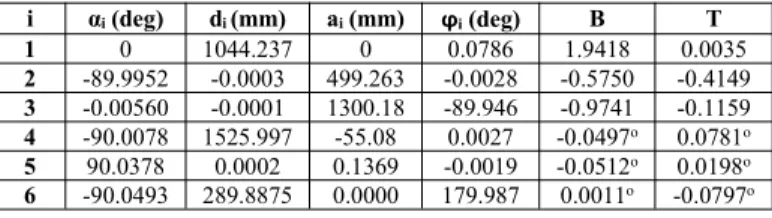
TABLE III. CALIBRATED PARAMETERS OF THE ROBOT

i αi(deg) di(mm) ai(mm) ϕi(deg) B T 1 0 1044.237 0 0.0786 1.9418 0.0035 2 -89.9952 -0.0003 499.263 -0.0028 -0.5750 -0.4149 3 -0.00560 -0.0001 1300.18 -89.946 -0.9741 -0.1159 4 -90.0078 1525.997 -55.08 0.0027 -0.0497o _0.0781o 5 90.0378 0.0002 0.1369 -0.0019 -0.0512o _0.0198o 6 -90.0493 289.8875 0.0000 179.987 0.0011o _-0.0797o

IV. VALIDATION PHASE

The second set of measured points is not used in the calibration phase. Since the new, calibrated robot’s parameters are obtained, they can be used to estimate the error for the both set of points – points for calibration phase and points for

validation phase. If they are similar, calibrated robot’s parameters could be used to predict the total displacement error for any point in the robot’s workspace, and compensate these errors.

It is expected to obtain smaller error for the set of points for calibration phase compared to estimated error for the set of points for validation phase, since the first set of points is used in the optimization procedure. It is important, that difference to be insignificant.

Computer-based simulation is performed such that the same machine coordinates are used in the forward kinematics procedure to calculate the tool position, but this time using the calibrated robot’s parameter. That way, the new nominal positions (1) are obtained and estimated error (3) is recalculated using the same measured positions (2).

The results of the simulation are given in Table 4.

TABLE IV. ESTIMATED ERROR USING SIMULATION

Calibration phase

points Validation phasepoints

Mean (mm) 0.174 0.242

St. dev. 0.070 0.150

Max. (mm) 0.370 0.921

V. ALGORITHM VERIFICATION

A. Compensation procedure

For 75 points chosen and used in calibration phase, the following procedure is performed.

Machine coordinates of appropriate point are taken, as they were used in the calibration phase:



des des des des des des



des



1, ,



2, ,



3, ,



4, ,



5, ,



6,

θ 

These values are used as initial values in the numerical algorithm for obtaining the commanded machine coordinates. This numerical algorithm is iteratively calling the forward kinematic procedure, but using calibrated, instead of nominal robot’s parameters used in ideal case. If the tool position in ideal case is:

Pi,des= [Xi,des,Yi,des,Zi,des]T  the iterative procedure is performed until the new tool position is close to Pi,desunder some predefined tolerance. Such, desired coordinates (12) are changed and new, compensated machine coordinates are stored as commanded coordinates:



com com com com com com



com 



1, ,



2, ,



3, ,



4, ,



5, ,



6,

θ 

These commanded coordinates for all 75 points previously used in the calibration phase are used in the last phase – verification phase and the new, second measurement is performed in order to compare predicted and measured total displacement error for these positions.

(6)

B. Measurement after calibration - results ans comparison Under the same conditions, the second measurement is performed, but using the commanded coordinates (14). In the same manner, the collected data are transformed to be expressed with respect to ACS, using the same transformation matrixTrexplained in details in the section C.

Finally, estimated errors for the set of 75 points used in the calibration phase is calculated using (3), as a norm of the displacement error. The mean, standard deviation and maximum of these estimated errors is shown in Table 2.

TABLE V. ESTIMATED ERROR AFTER CALIBRATION

Verification phase points Mean (mm) _0.293 St. dev. _0.168 Max. (mm) _1.511

As a result, the mean of total displacement error is reduced from 1.619mm before calibration to 0.293mm after calibration. That is significant difference, so with the second measurement, the correctness of the explained robot calibration procedure is verified.

In the validation phase, the mean of the displacement error was predicted by computer-based simulation as 0.174 mm for the first set of points, and as 0.242 for the second set of points. Since obtained error is 0.293 mm in the verification phase, one can conclude there is no significant difference between the error predicted by simulation and measured one, so in order to save production time, the second measurement should not be performed and only computer-based simulation could be used for error prediction after calibration.

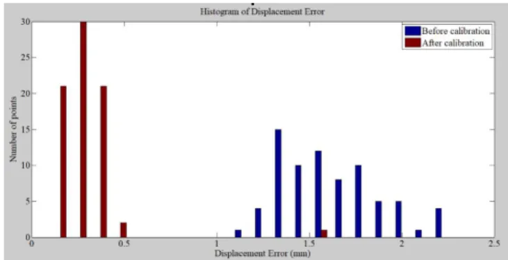
The histogram shown on Figure 2, shows the distribution of the displacement error before and after performing the calibration procedure.

Fig. 2. Histogram of displacement error before and after calibration

VI. CONCLUSION

This paper presented an algorithm for improving the accuracy of 6DOF industrial robot based on screw theory. This algorithm intended to improve the accuracy of the robot only by controlling the position of the robot’s end-effector.

Approximately 150 positions of the robot’s end-effector were measured using API laser tracker. Half of them were used to determine the calibrated parameters of the robot using an optimization process as a calibration method. The other half of the measured positions were used to estimate the correctness of the proposed calibration method.

Another measurement of the first set of 75 positions was performed in order to verify the correctness of the described calibration method and to checked if the value for the correctness of the calibration method determined in the validation phase is well estimated. From the results presented in this paper it can be seen that the proposed method improve the robot accuracy for more than 80% and that the validation phase gives good estimation for robot accuracy improvements with this calibration method, so the verification phase is not needed to be performed.

REFERENCES

[1] Xi F 1995 Effect of Non-Geometric Errors on Manipulator Inertial Calibration, IEEE International Conference on Robotics and Automation, Nagoya, Aichi, Japan, May 21-27, pp. 1808-1813

[2] Zhou J, Kang H-J 2015 A hybrid least-squares genetic algorithm-based algorithm for simultaneous identification of geometric errors in industrial robots, Advances in Mechanical Engineering7(6) 1-12, doi: 10.1177/1687814015590289

[3] Tao P Y, Yang G, Sun Y C, Tomizuka M, Lai C Y 2012 Product-Of-Exponential (POE) Model for Kinematic Calibration of Robots with Joint Compliance, IEEE/ASME International Conference on Advanced Intelligent Mechatronics, Kaohsiung, Taiwan, Jul. 11-14, pp. 496-501 [4] Jang J H, Kim S H, Kwak Y K 2001 Calibration of geometric and

non-geometric errors of an industrial robot, Robotica 19(3) 311-321, doi: 10.1017/S0263574700002976

[5] Kamali K, Joubair A, Bonev I A, Bigras P 2016 Elasto-geometrical calibration of an industrial robot under multidirectional external loads using a laser tracker, Robotics and Automation (ICRA), IEEE International Conference, Stockholm, Sweden, May 16-21, pp. 4320-4327

[6] Renders J M, Millan J R, Becquet M 1992 Non-Geometrical Parameters Identification for Robot Kinematic Calibration by use of Neural Network Techniques, In book: Tzafestas S G (eds) Robotic Systems. Microprocessor-Based and Intelligent Systems Engineering, 10 37-44, Springer, Dordrecht, doi: 10.1007/978-94-011-2526-0_5

[7] Samak S, Dimovski I, Dukovski V, Trompeska M 2016 Volumetric calibration for improving accuracy of AFP/ATL machines, 7th

International Scientific Conference on Defensive Technologies OTEH 2016, Belgrade, Serbia. Oct. 6-7, pp. 727-732

[8] Abderrahim M, Khamis A, Garrido S, Moreno L 2007 Accuracy and calibration issues of industrial manipulators, In book: Low K-H, (eds) Industrial Robotics–Programming, Simulation and Applications, pro literatur Verlag Robert Mayer-Scholz, Mammendorf, Germany, 131-146 [9] Lu D C-C, Hayes M J D 2013 Kinematic calibration of 6R serial

manipulators using relative measurements, CCToMM Mechanisms, Machines, and Mechatronics (M3_{) Symposium, Montréal, Québec, May}

30-31, pp. 151-162

[10] English K, Hayes M J D, Leitner M, Sallinger C 2002, Kinematic Calibration of Six-Axis Robots, CSME Forum, Kingston, Canada, May 21-24

[11] Švaco M, Šekoranja B, Šuligoj F, Jerebić B 2014 Calibration of an Industrial Robot using Stereo Vision System, Procedia Engineeding 69(2014) 459-463 (24th _{DAAAM International Symposium on}

Intelligent Manufacturing and Automation, 2013)

[12] Joubair A, Bonev I A 2015 Kinematic calibration of a six-axis serial robot using distance and sphere constraints,The International Journal of

(7)

Advanced Manufacturing Technology, 77(1-4) 515-523, doi: 10.1007/s00170-014-6448-5

[13] Liu B, Zhang F, Qu X 2015 A Method for Improving the Pose Accuracy of a Robot Manipulator Based on Multi-Sensor Combined Measurement and Data Fusion,Sensors,157933-7952, doi: 10.3390/s150407933 [14] Kihlman H, Loser R, von Arb K, Cooke A 2004Metrology-integrated

Industrial Robots – Clibration, Implementation and Testing, 35th

International Symposium on Robotics, Paris-Nord Villepinte, France, March 23-26

[15] Nguyen H-N, Zhou J, Kang H-L 2013 A New Full Pose Measurement Method for Robot Calibration, Sensors, 13 9132-9147, doi: 10.3390/s130709132

[16] Santolaria J, Conte J, Ginés M 2013 Laser-tracker-based kinematic parameter calibration of industrial robots by improved CPA method and active retroreflector, The International Journal of Advanced Manufacturing Technology, 66, 9-12 (2013) 2087-2106, doi: 10.1007/s00170-012-4484-6

[17] Dimovski I, Trompeska M, Samak S, Dukovski V, Cvetkoska D 2018 Algorithmic approach to geometric solution of generalized Paden– Kahan subproblem and its extension,International Journal of Advanced Robotic Systems,15(1) I-II, doi: 10.1177/1729881418755157

[18] Denavit J, Hartenberg R S 1955 A kinematic notation for lower-pair mechanisms based on matrices,J Appl Mech, 22, 215–221

View publication stats View publication stats