Washington University in St. Louis
Washington University Open Scholarship
Arts & Sciences Electronic Theses and Dissertations Arts & Sciences
Spring 5-18-2018
Variable selection via Lasso with high-dimensional
proteomic data
Hongxuan Zhai
Washington University in St. Louis
Follow this and additional works at:https://openscholarship.wustl.edu/art_sci_etds
Part of theStatistical Models Commons
This Thesis is brought to you for free and open access by the Arts & Sciences at Washington University Open Scholarship. It has been accepted for inclusion in Arts & Sciences Electronic Theses and Dissertations by an authorized administrator of Washington University Open Scholarship. For more
information, please [email protected].
Recommended Citation
Zhai, Hongxuan, "Variable selection via Lasso with high-dimensional proteomic data" (2018).Arts & Sciences Electronic Theses and
Dissertations. 1295.
WASHINGTON UNIVERSITY IN ST. LOUIS Department of Mathematics
Variable Selection via Lasso with High-dimensional Proteomic Data
by Hongxuan Zhai
A thesis presented to The Graduate School of Washington University in
partial fulfillment of the requirements for the degree
of Master of Art
May 2018 St. Louis, Missouri
Table of Contents
Page
List of Figures . . . iii
List of Tables . . . iv
Acknowledgments . . . v
ABSTRACT . . . vi
1 Introduction . . . 1
2 Statistical Models and Regulation Methods . . . 5
2.1 The Multinomial Logistic Model . . . 5
2.2 The Multinomial Logistic Model with Lasso and Elastic-Net Regulation . 6 2.3 The Uniqueness of Lasso Solutions and Optimization via Coordinate De-scent Algorithm . . . 7
2.4 Sparse Group Lasso . . . 12
2.5 Random Forest Classifier . . . 14
2.6 Support Vector Machine Classifier . . . 14
3 Data Analysis and Model Selection . . . 16
3.1 Check for Model Assumption . . . 16
3.2 Data Analysis Using Regularized Multinomial Logistic Regression with Lasso 17 3.3 Data Analysis using Sparse Group Lasso . . . 21
3.4 Bootstrapping for the tuning parameter . . . 22
3.5 Prediction accuracy and model comparison . . . 28
4 Conclusion . . . 30
A Some R code . . . 32
List of Figures
Figure Page
1.1 Overlay density plot for 10 samples . . . 3
3.1 Cross-validation plots for λopt . . . 18
3.2 Shrinkage effect of Lasso. . . 19
3.3 Coefficient Plot via Lasso. . . 20
3.4 Truncated version of grid search plot . . . 21
3.5 Shrinkage effect of elastic net. . . 22
3.6 Coefficient plot via elastic net. . . 24
3.8 Boostrapping for lambda in Lasso. . . 27
List of Tables
Table Page
1.1 Some features of the data. . . 4
3.1 Description of fitted models. . . 23
3.2 Confidence interval obtained by bootstrap. . . 26
Acknowledgments
I would like first to thank to my families. They supported me to finish my degree and they encouraged me while I studying abroad. I also want to thank my adviser, professor Kuffner, and he provided me with detailed guidance and resources. Thanks to all the professors who have taught me. From their teaching, I obtained knowledge and knew how to solve problems in scientific ways.
Hongxuan Zhai
Washington University in St. Louis May 2018
ABSTRACT
Variable Selection via Lasso with High-dimensional Proteomic Data by
Hongxuan Zhai A.M. in Statistics,
Washington University in St. Louis, 2018. Professor Todd Kuffner, Chair
Multiclass classification with high-dimensional data is an applied topic both in statis-tics and machine learning. The classification procedure could be done in various ways. In this thesis, we review the theory of the Lasso procedure which provides a parameter estimator while simultaneously achieving dimension reduction due to a property of the
`1 norm. Lasso with elastic net penalty and sparse group lasso are also reviewed. Our
data is high-dimensional proteomic data (iTRAQ ratios) of breast cancer patients with four subtypes of breast cancer. We use the multinomial logistic regression to train our classifier and use the false classification rates obtained from cross validation to compare models.
1. Introduction
The multinomial logistic model is frequently used in analysis of nominal multi-category response variables. The model can be regarded as a generalized linear model (GLM) with a logit link function. To estimate parameters in the multinomial logistic model, the maximum likelihood estimator (MLE) is typically used. However, MLE has the limitation that it will not provide a robust result when there are more parameters to be estimated than observations, or when some of the predictors are highly correlated. In both cases, MLEs’ tend to deteriorate rapidly. This has a negative effect on model interpretability. As a result, a variable selection procedure or dimension reduction procedure is needed to
obtain a more robust estimation result when the number of predictors,p, is much greater
than that of observations,n.
The Lasso, proposed by [1], is an acronym for Least Absolute Shrinkage and Selec-tion Operator, and it has become one of most popular methods for dealing with high-dimensional estimation problems. The data for our application study contains isobaric tags for relative and absolute quantitation (iTRAQ) proteome profiling of 77 breast can-cer samples and 3 duplicate breast cancan-cer samples generated by the Clinical Proteomic Tumor Analysis Consortium (NCI/NIH). The iTRAQ reporter ion intensity ratio is used to determine relative abundance of proteins within each sample. Data set contains expres-sion values for 12546 proteins for each sample, with missing values present when a given protein could not be quantified in a given sample. Relating to the proteomic data, the
response variable is sub-type of breast cancer given a certain sample. The proteomic data analyses is a "ratio-based" procedure, and the type of predictor variables are continuous while the type of response variable is categorical.
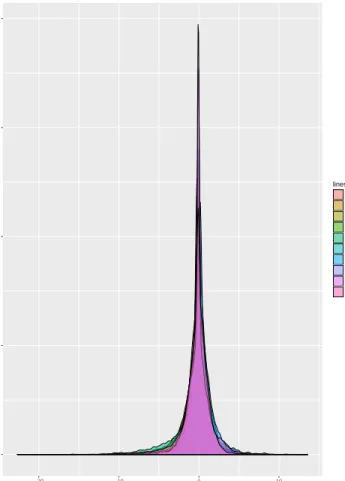
The data set is generated by an isobaric labeling method used in quantitative pro-teomics by Mass Spectrometry (MS) method, because proteomic analyses are performed on tumor fragments that are different from those used in genomic analysis, a pre-specified sample QC metrics are implemented. All the samples that do not exhibit a unimodal normal distribution are excluded from the study. The original experiment selected sam-ples for proteomic analyses from the subset annotated as having at least 130 mg wet weight residual material, the target amount for proteomics processing between collabo-rating research teams. After using this criterion, 131 sub-type samples were requisitioned from TCGA, including 28 basal, 20 HER2-enriched, 39 luminal A, and 39 Luminal B. 126 samples were obtained, of which 105 yielded at least the pre-specified minimum of 0.7 mg of total protein after extraction of proteins with 8M urea buffner. Among the 105 samples, there are 28 of tumor samples exhibiting highly skewed protein distribution. Finally, researchers obtain 77 tumor samples as well as 3 replicates that exhibited the expected gaussian unimodal distribution of a log iTRAQ ratio. It was assumed that for proteomic analyses tumor samples should be normalized samples with a log iTRAQ ratio centered at zero. As a result, a normalization scheme was employed that attempted to identify the unregulated proteins and centered the distribution of these log-ratios around zero in order to nullify the effect of systematic MS variation. There exist missing values in 77 samples, so an imputation is needed. In order to diminish the effect of outliers, we use the sample median to impute the missing values. Table (1.1) is the table describing
some features of the data and Figure (1.1) is the overlay density plot for 10 of the 80 samples to visualize the centered unimodal density.
0.00 0.25 0.50 0.75 1.00 −20 −10 0 10 dens density lines 1 10 2 3 4 5 6 7 8 9
Figure 1.1. Overlay density plot for 10 samples.
There are various well-established methods for variable selection. In the classical linear regression setup, forward/backward strategies have been utilized [2]. However, these methods are unstable and computationally costly [3]. For high-dimensional data,
wherepn, the ordinary least squares estimator (OLSE) is not unique and will heavily
overfit the data. Thus, regularized estimation of the regression coefficients is necessary.
When we focus on the regulation with`1 penalty, the parameters in linear regression are
Table 1.1
Some features of the data.
Variable predictor variables X response variables Y
number of observations 12546 77
variable type log-based continuous numeric ratio multi-categorical
models will be a convex optimization problem, which at the same time achieves variable
selection, because of the `1-geometry [1]. An alternative regularized regression method
is elastic net method that employs a combination of an `1 penalty and `2 penalty, which
is also a convex optimization [4]. Since both methods perform variable selection, we want to compare the performance of both methods for our proteomic data. The penalty parameter will greatly affect the model complexity. A large penalty parameter means that you will have zero or few variables in the model (a very sparse solution), while a small penalty parameter gets you closer to the least-squares solution (with as many predictors as can be estimated from n observations). We also need to do grid searches for the tuning parameters for the two selected methods under certain criterion. Therefore, we search for optimal values of the tuning parameters over a grid of candidate values, where optimality is defined in terms of mean square prediction error (MSPE). We will
2. Statistical Models and Regulation Methods
2.1 The Multinomial Logistic Model
The multinomial logistic regression model is a particular type of GLM [7] which allows for multi-category response variables, i.e. there are more than two categories for the response variable. Similar to the logistic model with binary response, the multinomial logistic model utilizes the logit link function to model the logarithm of the odds ratio as
the linear combination of predictor variables X = (X1, X2, ...Xp).Supposep is a random
variable taking values between 0 and 1; The logit link function is defined as
logit(p) = log( p
1−p);
Since the link function could be regarded as a transformation of the conditional mean
E(Y|X =x), it would naturally give rise to the context of regression. The linear logistic
regression model with multicategory response can be regarded as a generalization of the binary response linear logistic regression that extends one logit to multiple logits. Suppose
Y is a multicategory response withKlevels; A multinomial logistic model with predictors
X = (X1, X2, ...Xp) is defined as
log P r(Y =`|x)
P r(Y =K|x) =β0`+x
Tβ
`, ` = 1,2, ..., K−1,
where β`T = (βl1, ..., βlp) are the regression coefficients.
An equivalent but more symmetric parametrization [4]
P r(Y =`|x) = exp(β0`+x
Tβ `)
PK
Notice that this equivalent parametrization is not estimable since for parameters (β0`, β`),
a shifted version (β0`−a0, β`−a) will generate the same probability measure. The
non-estimable property will also make the log-likelihood insensitive to the shifting constant
(a0, a) when we do maximum likelihood estimation [8].
2.2 The Multinomial Logistic Model with Lasso and Elastic-Net Regulation
In the classical linear model context, given a collection of N samples (xi, yi)Ni=1, the
Lasso method finds the solution (βˆ
0,βˆ) of the optimization problem defined by
minimize β0,β 1 2N N X i=1 (yi−β0− p X j=1 xijβj)2 subject to p X j=1 |βj| ≤t;
Notice that the constraint could also be written as ||β||1 ≤ t, where k · k denotes the
`1 norm. Due to Lagrangian duality, the minimization procedure could also be in a
Lagrangian form, defined by
minimize β0,β 1 2N N X i=1 (yi−β0− p X j=1 xijβj)2+λ||β||1,
for someλ≥0. There exists a one-to-one mapping between the solutions for the two
con-strained problems. In a multinomial logistic regression setup, the negative log-likelihood
with `1 penalization is given by
−1 N N X i=1 log(P r(Y =yi|xi; (β0, βk)Kk=1) +λ K X k=1 ||βk||1,
where βk is a vector with components β1k, . . . , βpk, and that the different βk correspond
to the vectors of coefficients for the K different classes for the response. Since the
with respect to a constant shift of K coefficients, the penalty function is not invariant
with respect to a constant shift coefficients [9]. Penalty term could resolve the choice of
cj when{βkj+cj} and {βkj} generate same probability from the likelihood function. As
a result, the optimal choice cj for each candidate set {βkj}Kk=1 could be generated by
argmin c∈R K X k=1 |βkj−c|
and it can be shown that the solution of the objective is the median of {βˆ1j, ...,βˆKj} for
eachj = 1, ..., p.
Estimation of the multinomial logistic model via elastic net corresponds to a penalized estimation problem of the form
minimize β0,β −1 N log(P r(Y =yi|xi; (β0, βk) K k=1) +λ p X j=1 ρj(1−α)βj2+ρjα|βj|.
This penalty could be regarded as a compromise between `1 and `2 penalty (also known
as ridge penalty) and this penalty is particularly useful in the p N situation [4]. The
parameter αis a real number between 0 and 1 serving as the weighting parameter of the
Lasso penalty and ρj is non-negative quantity serving as a penalty modifier. Notice that
elastic net penalty is convex, and hence we can employ convex optimization methods.
2.3 The Uniqueness of Lasso Solutions and Optimization via Coordinate Descent Algorithm
The Lasso estimator is the solution of the optimization problem
minimize β0,β 1 2N N X i=1 (yi−β0− p X j=1 xijβj)2
subject to
p
X
j=1
|βj| ≤t;
It is known that the solution is unique when the rank of the X matrix is equal to the
number of columns. Notice that in high-dimensional data analysis, we have data sets where the number of variables exceeds the number of observations. As a result, the Lasso
criterion is not strictly convex and there are infinitely many solutions, βˆ, that yield a
perfect fit with zero training error. This leads to instability in the estimates, even though
the fitted values of Xβˆare unique. For illustration, consider one simple example where
x1 and x2 are predictor variables and y is the response variable, and suppose the Lasso
solution βˆ at a certain λ is ( ˆβ1,βˆ2). If there is an additional predictor x3 = x2 in the
model, any vector satisfying βˆ(α) = ( ˆβ
1, αβˆ2,(1−α) ˆβ2) for α∈[0,1] produces the same
model fit and has the same`1norm. Obviously, in this example, there are infinitely many
solutions.
The columns of the matrix X are said to be in general position if for {xj}pj=1, any
affine subspace L in RN of dimension k < N contains at most k+ 1elements of the set
{±x1,±x2, ...,±x3}, excluding antipodal pairs of points. An affine space is a geometric
structure that generalizes the properties of Euclidean spaces in such a way that these are independent of the concepts of distance and measure of angles, keeping only the properties related to parallelism and ratio of lengths for parallel line segments. In a high-dimensional data setting, one can show that if the predictor variables are drawn from a
continuous probability distribution, then with probability one, the columns of X are in
For a general differentiable convex function f with convex constraint set C ∈ Rp ,
consider the constrained optimization problem defined by
minimize
β∈Rp f(β) such that β ∈C;
A necessary and sufficient condition for a vector β∗ ∈Cto be a global optimum is that
<5f(β∗), β−β∗ >≥ 0;
When the constraint set Ccan be described as sublevel sets of certain convex constraint
functions g : Rp →
R, the convex optimization problem can be written in the form of
minimize β∈Rp
f(β) such that gj(β) ≥ 0 f or j= 1, ..., m;
The Lagrangian associated with this problem is
L(β, λ) =f(β) +
m
X
j=1
λjgj(β),
where the weights λ ≥ 0 are Lagrange multipliers. Under technical conditions on f
and gi, Lagrangian duality guarantees the existence of an optimal choice of λ∗. The
necessary and sufficient conditions for finding the global optimum β∗ related to λ∗ are
the Karush-Kuhn-Tucker (KKT) conditions.
The Lasso problem involves the `1 norm, and hence the objective function fails to be
differentiable when any of the coordinates βj is exactly equal to zero. In this situation,
the KKT conditions are not directly applicable but there is a generalized notion of the gradient called the subgradient. Based on the property that for a differentiable convex function the first-order tangent approximation always provides a lower bound, the notion
of a subgradient of function f atβ is defined as a vector z ∈Rp such that
The set of all subgradients off atβ is called the sub-differential, denoted by∂f(β). For
absolute value functionf(β) =|β|, we define
∂f(β) = 1, if β is greater than 0 −1, if β is less than 0 [−1,1], if β is 0
We will use the notation that z ∈sign(β) to express the idea thatz belongs to the
sub-differential of the absolute value function at β.As a result, the first-order condition, i.e.
the requirement that the gradient is zero for an optimal solution, can be generalized to a condition involving the sub-differential,
0∈∂f(β∗) + m
X
j=1
λ∗j∂gj(β∗);
Applying this to the Lasso problem, we have the constraint functiong specified asg(β) =
Pp
j=1|βj| −R for some positive R. Numerical methods are needed to solve such an
optimization problem. Newton’s method as a second-order method that using knowledge of Hessian, not just first derivative, has a quadratic rate of convergence; However Newton’s method has lower computation efficiency. Especially in the multinomial regression setup, newton’s method can be tedious. Coordinate descent method is an iterative algorithm
that updates parameter β by choosing a single coordinate, and then doing a univariate
minimization over the chosen coordinate using first-order method [9]. To be more specific,
suppose coordinate k is chosen at iteration t; The update for the chosen coordinate is
given by βkt+1 = argmin βk f(β1t, β2t, β3t, ..., βk, βkt+1, ..., β t p),
and βjt+1 = βt
j for j 6= k. This algorithm solves the optimization problem by cycling
through the coordinates in a particular fixed order. One sufficient condition for
conver-gence to the global minimum is that functionf is continuously differentiable and strictly
convex with respect to each coordinate. It is obvious that when using the`1norm penalty,
this restrictive condition is not satisfied. In such cases, a separability condition will en-sure that coordinate-wise minimization algorithms do not get stuck at sub-optimal values.
The separability condition for a cost function f is defined as an additive decomposition
f(β1, ..., βp) = g(β1, ..., βp) +
p
X
j=1
hj(βj),
where function g : Rp → R is differentiable and convex, while any of the univariate
functions hj : R → R are convex. [11] shows that for any convex cost function f with
separable structure, the coordinate descent algorithm is guaranteed to converge to the global minimizer.
The coordinate descent method is implemented in regularized multinomial regression to get the estimate of coefficients. Followed by [8], the optimization procedure utilizes both partial Newton steps by forming a partial quadratic approximation and the coor-dinate descent method. As a generalization for regularized logistic regression of binary response, we model the multinomial case by
P r(Y =`|x) = exp(β0`+x
Tβ `)
PK
k=1exp(β0k+xTβk)
suggested by [4]. Here the corresponding likelihood function becomes regularized
max-imum multinomial likelihood. We suppose the categorical response variables to be G,
be the indicator response matrix with yi`=I(gi =`), the explicit form of unregularized log-likelihood is given by `({β0`, β`} K 1 ) = 1 N N X i=1 [ K X `=1 yi`(β0`+xiTβ`−log( K X `=1 eβ0`+xiTβ`)].
First, we utilize partial Newton steps by performing a partial quadratic approximation to the unregularized log-likelihood and get
`Q`(β0`, β`) =− 1 2N N X i=1 wi`(zi`−β0`−xiTβ`) 2 +C({β0k, βk}K1 ) where zi`= ˜β0`+xiTβ˜`+ yi`−p˜`(xi) ˜ p`(xi)(1−p˜`(xi)) wi`= ˜p`(xi)(1−p˜`(xi))
Second, we utilize the current parameter estimates( ˜β0,β˜) and coordinate descent
algo-rithm to solve the problem with penalization, which allows only one element in (β0`, β`)
to vary at a time. The problem is described as
minimize β0`,β`
{−`Q`(β0`, β`) +λPα(β`)}.
2.4 Sparse Group Lasso
The sparse group lasso method is a combination between the lasso [1] and the group lasso [12]. The sparse group lasso also utilizes a gradient descent method to find the solution to the optimization problem. In the multiclass classification setting, the sparse group lasso method based on a multinomial regression model takes the structured feature of parameters into consideration and generally improves the performance of the classifier in the high-dimensional setting [13]. Compared to the Lasso or group Lasso, the sparse group Lasso also substantially reduces the number of selected variables.
Consider we have p features and we decompose the search space in to m blocks
Rp =Rp1 ×...×Rpm
wherepi is the dimension of the group i, with p=p1+p2+..+pm. For coefficient vector
β we have β = (β(1), ..., β(m))where β(1) ∈Rp1, ..., β(m) ∈Rpm. The subvectorβ(J) is the
Jth block of β for J = 1, ..., m, and we denoteβJ
i as the ith coordinate of the Jth block
of coefficients.
The sparse group lasso penalty is defined as
Φ(β) = (1−α) m X J=1 γJ||β(J)||2+α p X i=1 ξi|βi|,
where α ∈ [0,1], γ ∈ [0,∞)m are the group weights, and parameter weights ξ =
(ξ(1), ..., ξ(m)) ∈ [0,∞)p for ξ(1) ∈ [0,∞)p1
, ..., ξ(m) ∈ [0,∞)pm. As with the elastic net
method, the tuning parameter α could lead to two different methods by taking α = 1
(lasso penalty) or α= 0 (group lasso penalty).
The multinomial sparse group lasso classifier problem with K classes,N samples and
p features has the N × p design matrix X = (x1, ..., xN)T and yi ∈ {1, ..., K} is the
categorical response. A symmetric parametrization is used in sparse group lasso with
loss function h(l, η) = exp(η1)
PK
k=1exp(ηk)
; Together with this penalty function, the sparse
group lasso problem is expressed as a penalized likelihood criterion, − N X i=1 log(h(yi, β(0)+βxi)) +λ((1−α) p X J=1 γJ||β(J)||2+α Kp X i=1 ξi|βi|);
For computational aspect, the R package msglcitepmsgl uses a decreasing sequence of λ
2.5 Random Forest Classifier
Decision trees are a non-parametric supervised learning algorithm used for regression and classification. The goal is to create a model that predicts the value of a target variable by learning simple decision rules inferred from the data features. Given an input which is usually represented by a feature vector, decision trees make prediction according to function in hypothesis space. Decision trees’ performance can be evaluated based on mean square error and mean square prediction error. Given a data, one could use bootstrap scheme to establish multiple decision trees, which is called a random forest. The random forest classifier is defined by {h(x,Θk), k = 1, ...} where Θk are independent identically
distributed random vectors and each tree casts a unit vote for the most "popular" class
at each input x [14]. Random forests are composite methods that consist of decision
trees generated by bootstrapping training data. The variables at each node are random subsets of the full set of predictor variables, and also each node and the number of nodes in the decision tree are generated randomly. All the decision trees can be grown to the
desired size. A large number of trees are generated based onB bootstrap samples fromn
samples and vote for the most popular class, and such procedure is called random forest.
2.6 Support Vector Machine Classifier
Support vector machines (SVMs) are supervised classification methods which utilize separating hyperplanes. Given a training dataset with pre-specified labels, SVMs give classification outputs based on an optimal hyperplane computed by categorizing new data points. Classical SVMs achieve separation between two classes by making use of a
hyperplane is equivalent to solving the following optimization problem in Lagrangian form: L(w, b, α) = 1 2||w|| 2 − n X i=1 αi[yi(wTxi+b)−1];
Based on the optimumw∗, b∗, α∗, we can obtain the optimal hyperplane, which is defined
by w∗Tx+b∗ = 0. With each input vector x, outputs are calculated by the function
sign(w∗Tx +b∗); Multiclass SVMs are a multiclass generalization of SVMs for binary
classification. Multiclass SVM builds and combines several binary class SVMs classifiers, and hence is more computational expensive than binary class SVMs. This method is
called the one-against-one method. The procedure buildsk(k−1)/2classifiers, with each
classifier trained on data obtained from any two classes. The classification problem is
defined by minimizing over w, b, ξ
1 2(w ij)Twij +CX t ξijt , subject to (wij)Tφ(xt) +bij ≥1−ξtij, if yt =i (wij)Tφ(xt) +bij ≤ −1 +ξtij, if yt=j ξtij ≥0, where CP tξ ij
t is the penalty term, and training data is from ith and jth classes. The
3. Data Analysis and Model Selection
3.1 Check for Model Assumption
One main feature of Lasso regression is that Lasso regression will do variable selection and model fitting at the same time; However, Lasso regression is also notoriously known as its instability. As a result, we need to further investigate the credibility of our selection algorithm and how stable are our findings so that we could have a more efficient and reasonable statistical procedure. First, we describe the variable selection procedure for Lasso to be
ˆ
S(λ) = {j; ˆβj(λ)6= 0}
f or S0 ={j;βj0 6= 0},
where Sˆ(λ) could be regarded as the selected non-zero coefficient set and S0 could be
regarded as the true non-zero coefficient set. If a variable selection procedure performs well, we expect that there is high probability that the two sets are essentially equal. In order to get a stable solution in Lasso regression, some conditions and problems are worth considering.
• Neighborhood stability condition is restrictive
• Choice of λ will affect the selection of variables
Among these conditions and problems, the neighborhood stability condition is restric-tive, and it is also a sufficient and necessary condition for consistent model selection with
Lasso. For a matrix X, the neighborhood stability condition is that ,in terms of
sub-matrices, there is no strong linear dependence. Since in Lasso regression, the regression
coefficients are function of the chosen λ, Empirically, λ is chosen to be λopt defined as
λopt = argmin λ E (Y − p X j=1 ˆ βj(λ)X(j))2;
It can be shown that for prediction optimalλopt
ˆ
S(λopt)⊇S0,
which means that the true active set is contained in the estimated active set including the selected variables. This is the screening feature of Lasso regression. Considering our
data, the design matrixX has some correlated columns but not strongly correlated since
the number of correlated columns is much smaller than the total number of columns. The motivating data satisfy the neighborhood stability condition.
3.2 Data Analysis Using Regularized Multinomial Logistic Regression with Lasso
We label the four breast cancer sub-types (Luminal A, Luminal B, Basal-like, and HER2-enriched) with categorical variables 1 to 4 and treat them as the response variable
with respect to each sample. We first choose the tuning parameterλin the Lasso penalty
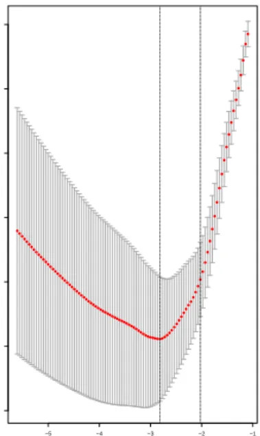
using cross-validation procedure and chooseλoptto be the one that minimize the deviance
with respect to multinomial logistic regression. The cross-validation plot is generated
prediction oracle. We could also see the obvious shrinkage effect of Lasso regression −5 −4 −3 −2 −1 1.6 1.8 2.0 2.2 2.4 2.6 2.8 log(Lambda) Multinomial De viance 272625262524242321191816151412865310
Figure 3.1. Cross-validation plots for λopt.
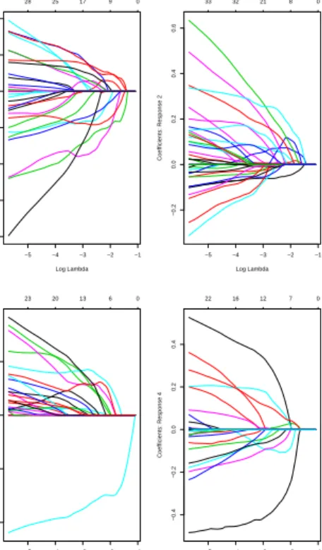
with increment of λ in figure (3.2). Larger value of λ will eliminate more variables in
the model. Utilizing theλopt via cross-validation to fit the multinomial logistic model by
coordinate descent algorithm, we will do both variable selection and model fitting in one
statistical procedure. Notice thatglmnetpackage uses the "redundant" parameterization
of multinomial logistic regression. As a result, we will get 4 groups of selected variables
and their corresponding coefficients. It is obvious that under λopt, the dimension of the
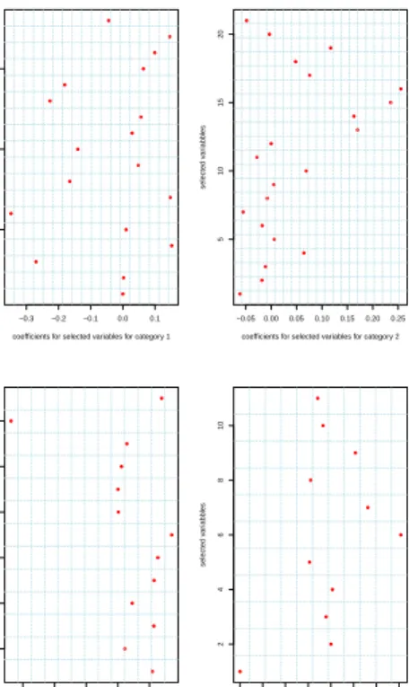
regression problem is greatly reduced. From each category, Lasso regression select 18, 21, 13, 11 variables respectively. As suggested by [8], the intercept coefficients are always not penalized. So that in each model for a certain category, there is always an intercept term. Figure (3.3) displays the coefficient plot for Lasso.
It is worth mentioning that Lasso method is insensitive to the highly correlated data
−5 −4 −3 −2 −1 −0.8 −0.6 −0.4 −0.2 0.0 0.2 0.4 Log Lambda Coefficients: Response 1 28 25 17 9 0 −5 −4 −3 −2 −1 −0.2 0.0 0.2 0.4 0.6 Log Lambda Coefficients: Response 2 33 32 21 8 0 −5 −4 −3 −2 −1 −0.4 −0.2 0.0 0.2 Log Lambda Coefficients: Response 3 23 20 13 6 0 −5 −4 −3 −2 −1 −0.4 −0.2 0.0 0.2 0.4 Log Lambda Coefficients: Response 4 22 16 12 7 0
Figure 3.2. Shrinkage effect of Lasso and coefficient path.
variables from correlated variables, which leads us to do a multinomial regression pro-cedure using a different penalty function-elastic net method. In order to get the best tuning parameters in elasticnet model, we need to do a grid search over both the elastic
net mixing parameter α and the penalized parameterλ. Since the elastic net mixing
pa-rameter α ∈[0,1], we only need to have an reasonable interval from which we can have
an efficient search over penalized parameterλ.A theorem related to the variable selection
with Lasso suggests that under some conditions, some choices of λ will lead to a good
variable selection procedure. These conditions are described as:
• the design matrix satisfy the neighborhood stability condition [15] • data has high-dimensionality
−0.3 −0.2 −0.1 0.0 0.1
5
10
15
coefficients for selected variables for category 1
selected v ar iab b les −0.050.00 0.05 0.10 0.15 0.20 0.25 5 10 15 20
coefficients for selected variables for category 2
selected v ar iab b les −0.3 −0.2 −0.1 0.0 0.1 2 4 6 8 10 12
coefficients for selected variables for category 3
selected v ar iab b les −0.4−0.3−0.2−0.1 0.0 0.1 0.2 0.3 2 4 6 8 10
coefficients for selected variables for category 4
selected v
ar
iab
b
les
Figure 3.3. Coefficient Plot via Lasso.
• the estimated active set has sparsity Then if λ =λn∼n− 1 2− δ 2(0< δ < 1 2)
P[ ˆS(λ) =S0]1 even f or relatively small n;
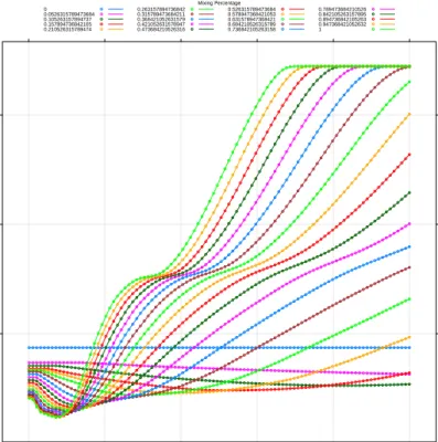
This gives us a tentative guide for the search interval. Figure (3.4) shows the truncated
graph of the grid search with respect to penalized parameterλ under different elasticnet
mixing parameter α. After the grid search using the repeated cross-validation criterion,
we get the tuning parameters to be α = 0.24242 and λ = 0.08636 respectively. The
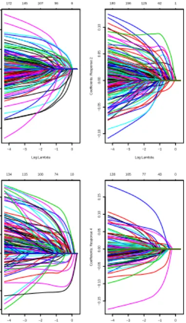
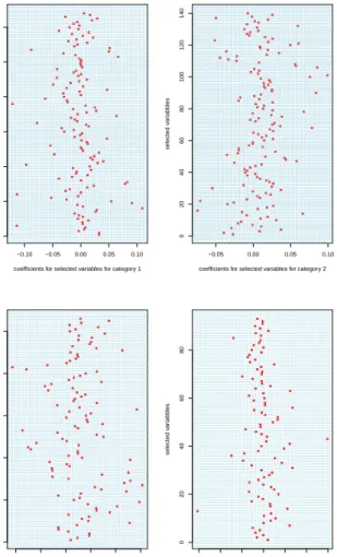
regression with elasticnet selects 128, 140, 106, 93 variables (include the unpenalized intercept term) respectively for each category. Figure (3.5) illustrate the relative shrinkage
effect of elasticnet, from which we conclude that elasticnet method tend to select more variables into the model. Figure (3.6) displays the coefficient plot for elasticnet.
Regularization Parameter
RMSE (Repeated Cross−V
alidation) 0.8 0.9 1.0 0.0 0.2 0.4 0.6 0.8 1.0 Mixing Percentage 0 0.0526315789473684 0.105263157894737 0.157894736842105 0.210526315789474 0.263157894736842 0.315789473684211 0.368421052631579 0.421052631578947 0.473684210526316 0.526315789473684 0.578947368421053 0.631578947368421 0.684210526315789 0.736842105263158 0.789473684210526 0.842105263157895 0.894736842105263 0.947368421052632 1
Figure 3.4. Truncated version of grid search plot.
3.3 Data Analysis using Sparse Group Lasso
R package msgl allows users to fit a multinomial logistic regression with sparse group
lasso penalty with a sequence of tuning parameters λ. With this setting, users need to
prespecify a minimum value of sequence of λ. In this thesis, we set the minimum of
sequence of λ to be 0.05, hence msgl fit the model with whole data with a λ sequence
ranging from 0.22 to 0.05. The fitted models description is shown in the table. Through-out the table, one can clearly see the sparsity of coefficients of sparse group lasso method based on the number of selected features and the number of estimated parameters. To get
−4 −3 −2 −1 0 −0.15 −0.10 −0.05 0.00 0.05 0.10 0.15 Log Lambda Coefficients: Response 1 172 145 107 56 6 −4 −3 −2 −1 0 −0.10 −0.05 0.00 0.05 0.10 Log Lambda Coefficients: Response 2 180 156 125 62 1 −4 −3 −2 −1 0 −0.06 −0.04 −0.02 0.00 0.02 0.04 0.06 Log Lambda Coefficients: Response 3 134 115 100 74 10 −4 −3 −2 −1 0 −0.15 −0.10 −0.05 0.00 0.05 0.10 0.15 Log Lambda Coefficients: Response 4 128 105 77 43 0
Figure 3.5. Shrinkage effect of elastic net and coefficient path.
the best tuning parameter λ, like the previous method, we do a 10-fold cross validation
to select the best tuning parameter. Also for the mean square prediction error of this method, 10-fold cross validation is used and an average is taken among the mean square prediction error.
3.4 Bootstrapping for the tuning parameter
The bootstrap method can provide us with some statistical inference about the es-timated parameters when there is little prior information about the distribution of the parameters. The nonparametric resampling method is based on resampling the observed data with replacement. The vector resampling is one method of nonparametric bootstrap that generates the new data as a sample from a certain bivariate distribution. Consid-ering acquiring the distribution of tuning parameters, we have the bootstrap procedure designed as the follow,
Table 3.1
Description of fitted models.
Index lambda features Parameters
1 1.00 1 4 20 0.75 6 17 40 0.55 22 55 60 0.41 31 75 80 0.30 50 117 100 0.22 57 135
−0.10 −0.05 0.00 0.05 0.10 0 20 40 60 80 100 120
coefficients for selected variables for category 1
selected v ar iab b les −0.05 0.00 0.05 0.10 0 20 40 60 80 100 120 140
coefficients for selected variables for category 2
selected v ar iab b les −0.04 −0.02 0.00 0.02 0.04 0.06 0 20 40 60 80 100
coefficients for selected variables for category 3
selected v ar iab b les −0.15 −0.10−0.05 0.00 0.05 0.10 0.15 0 20 40 60 80
coefficients for selected variables for category 4
selected v
ar
iab
b
les
Figure 3.6. Coefficient plot via elastic net.
• Sampling with replacement from the original data set of (X,Y), and generate
boot-strapped pairs and combine them as the bootboot-strapped sample
• Based on the bootstrapped sample, get the best estimate for the tuning parameters • Repeat step one and step two
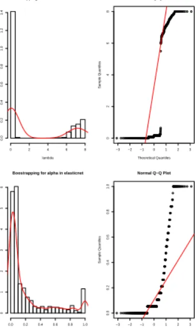
Based on this statistical procedure, we obtain the sample distribution for the tuning parameters under both "Lasso" model and "elastic net" model that are displayed as fig-ure(3.7) and figure(3.8). Through the Q-Q plots of the estimates for tuning parameters,
0 2000 4000 6000 8000 10000 12000 −1 0 1 2 3 variable number Impor tance
Variable Importance for 4 Levels of Response
type= 1 type= 2 type= 3 type= 4
we can conclude that in "Lasso" model the sample distributions for both λmin and λ1se
are asymptotic normal. However, the sample distributions for tuning parameters α and
λ in elastic net model are highly skewed and do not display normal distribution
charac-teristics. As a results the bootstrap confidence interval for those tuning parameters are constructed under different assumptions. For the tuning parameters of "Lasso" model, we construct such interval based on the asymptotic normal-distributed feature of the sample distribution while for the tuning parameters in "elastic net" model we use the percentile method. The confidence intervals are described as table (3.2)
It is worth mentioning that based on the bootstrap method, λopt obtained by cross
validation does not lie in the confidence interval ofλopt obtained by bootstrap resampling
but it does lies in the confidence interval ofλ−1se. And for "elastic net" model, bootstrap
Table 3.2
Confidence interval obtained by bootstrap.
Lasso:λopt Lasso:λ1se Elsticnet:λ Elsticnet:α
the confidence interval obtained by bootstrap method. It may be conclude that the basic bootstrap method under the brute-force searching algorithm does not yield relatively satisfying results in the context of statistics for high-dimensional data.
Boostrapping for lambdamin in Lasso
lambdamin Density 0.00 0.01 0.02 0.03 0.04 0.05 0 10 20 30 40 50 −3 −2 −1 0 1 2 3 0.01 0.02 0.03 0.04 Normal Q−Q Plot Theoretical Quantiles Sample Quantiles
Boostrapping for lambda1se in Lasso
lambda1se Density 0.020.040.060.080.100.120.14 0 5 10 15 −3 −2 −1 0 1 2 3 0.02 0.04 0.06 0.08 0.10 0.12 0.14 Normal Q−Q Plot Theoretical Quantiles Sample Quantiles
Figure 3.8. Boostrapping for lambda in Lasso.
Boostrapping for lambda in elasticnet
lambda Density 0 2 4 6 8 0.0 0.2 0.4 0.6 0.8 1.0 1.2 1.4 −3 −2 −1 0 1 2 3 0 2 4 6 8 Normal Q−Q Plot Theoretical Quantiles Sample Quantiles
Boostrapping for alpha in elasticnet
alpha Density 0.0 0.2 0.4 0.6 0.8 1.0 0 1 2 3 4 5 6 −3 −2 −1 0 1 2 3 0.0 0.2 0.4 0.6 0.8 1.0 Normal Q−Q Plot Theoretical Quantiles Sample Quantiles
3.5 Prediction accuracy and model comparison
Since both regressions with Lasso or elastic net are optimization problems, we have relative fewer criterion to test that whether the fitted model is good. One criterion that we can use is the false classification rate of the fitted model. Table (3.3) shows the false classification rate for 5 methods of classification in high dimensional data setup. In terms of prediction accuracy, we use 10 fold cross validation to get the false classification rate. Under our motivated data, the multinomial logistic regression model with sparse group lasso has the best prediction accuracy, and multinomial logistic regression models with lasso and elastic net are less powerful in prediction compared with the previous model. Based on these corresponding results, multinomial logistic regression model with Lasso provide us with a better fit and a more parsimonious model since Lasso method selects less variables into the model compared to elastic net method. Due to the fundamental
difference between `1 geometry and `2 geometry, under certain choice of λ, the Lasso
method could guarantee that the coefficients of some groups of variables are exactly zero. But there are also some issues regarding the criterion and procedure for model selec-tion and model predicselec-tion. First, the false classificaselec-tion rate could be sensitive to the sample size. In our motivated data, since there are 77 different samples that is relatively small, the false classification rate might not be representative enough. Second, since in general the problem of Lasso could be regarded as optimization problem that yield little statistical test like confidence interval and p-value, we have relatively less information to combine Lasso with classic statistical test. As a result, we have less information about the uncertainty of our selected model and hypothesis testing, and the most direct message we can utilize is the prediction power of our model. Third, since the prediction error is
Table 3.3
False classification rate.
Lasso:λopt Elsticnet:λopt Sparse group lasso random forest SVMs 25.3% 27.5% 24.5% 29.2% 30.2%
almost zero with Lasso method, we can not rule out the possibility of overfitting phe-nomenon. Also, in the aspect of optimization algorithm, there exists no test regarding the convergence.
glmnetpointed out that the code provided inglmnetpackage does not implement any checks for divergence, since this check would slow down the computing for the solution, where the fast speed of computation with coordinate descent is the main advantage against other optimization algorithm. The coordinate descent algorithm have a closed form of expression for the starting solutions and subsequent solutions are warm-started from the previous close-by solutions that generally make the quadratic approximations very accurate. There is no documented example of divergence problem so far.
4. Conclusion
In this thesis, we review basic theory of lasso (least absolute shrinkage and selection oper-ator) regression method and its generalization method that is elastic net. We utilize such methods to analyze our motivated data that is really a high-dimensional data with the number of predictors is much greater than the number of samples. Both methods per-form an obvious dimension-reduction effect and overcome some drawbacks that ordinary least square method and maximum likelihood estimator intrinsically have. In theory, the
property of `1 geometry guarantee that the Lasso method could do the variable
selec-tion and model fitting at the same time, and the elastic net method as an compromise between Lasso and ridge regression method could also serve as a variable selection pro-cedure. Under Lasso and elastic net regression method, the fitted models based on our motivated data display different complexity. The model fitted by Lasso tends to select fewer variables compared to the model fitted by elastic net, in which Lasso provides us with a more parsimonious model. Considering the model selection criterion based on pre-diction accuracy, Lasso outperforms elastic net method in the analysis of our motivated data. The best model with smallest false classification rate is multiclass logistic regres-sion with sparse group lasso penalty that allows sparsity within each selected feature. Our motivated data has very few samples but huge number of features, and it is highly possible that among those features exist large amounts of noises. Since all the penalized regression methods have relatively high false classification rate, we also utilized machine
learning algorithms to compare models. It turns out that machine learning methods pro-vides us with an even worse classification power. Thus, the penalized regression methods (Lasso, elastic net, and sparse group lasso) achieve performance and results as good as possible. Also the basic bootstrap method for getting the confidence interval for tuning parameter does not yield good results and in the future I want to investigate more about the construction of confidence interval for statistical model based on high-dimensional data and do more post inference in statistics for high-dimensional data.
A. Some R code
Lasso: Fold = f u n c t i o n ( Z =10 , w , D , seed = 7 7 7 7 ) { n = nrow ( w ) d =1: n ; dd = list () e = l e v e l s ( w [ , D ])T = l e n g t h ( e ); set . seed ( seed ) for ( i in 1: T ){ d0 = d [ w [ , D ]== e [ i ]]; j = l e n g t h ( d0 ) ZT = rep (1: Z , c e i l i n g ( j / Z ) ) [ 1 : j ] id = c b i n d ( s a m p l e ( ZT , l e n g t h ( ZT )) , d0 ); dd [[ i ]]= id } mm = list (); for ( i in 1: Z ) { u = NULL ; for ( j in 1: T ) u = c ( u , dd [[ j ]][ dd [[ j ]][ ,1]== i ,2]) mm [[ i ]]= u } r e t u r n ( mm )} # g e n e r a t e c r o s s v a l i d a t i o n set w = read . csv ( file = " / U s e r s / t e k i n o s e i / D o w n l o a d s / d a t a 1 ␣ (1). csv " , h e a d e r = TRUE , sep = " , " ) w = w [ , -1] con <- as . f a c t o r ( w [ , 1 2 5 4 7 ] ) w = w [ , -12547]
w = c b i n d ( w , con ) # load data # 10 - fold CV l i b r a r y ( g l m n e t ) D = 1 2 5 4 7 ; Z =10; n = nrow ( w ); mm = Fold ( Z , w , D , 1 2 0 2 ) Z =10 E = rep (0 , Z ) for ( i in 1: Z ){ m = mm [[ i ]] n1 = l e n g t h ( m ) w1 <- as . m a t r i x ( w [ , -12547]) c v l a m b d a <- cv . g l m n e t ( w1 [ - m ,] , w [ - m , D ] , f a m i l y = " m u l t i n o m i a l " )
a = p r e d i c t ( cvlambda , newx = w1 [ m ,] , s = c v l a m b d a $ l a m b d a . min , type = " c l a s s " ) E [ i ]= sum ( w [ m , D ] ! = a ) / n1 show ( i )} mean ( E ) Elastic-net: l i b r a r y ( g l m n e t ) Fold = f u n c t i o n ( Z =10 , w , D , seed = 7 7 7 7 ) { n = nrow ( w ) d =1: n ; dd = list () e = l e v e l s ( w [ , D ])
T = l e n g t h ( e ); set . seed ( seed ) for ( i in 1: T ){
d0 = d [ w [ , D ]== e [ i ]]; j = l e n g t h ( d0 ) ZT = rep (1: Z , c e i l i n g ( j / Z ) ) [ 1 : j ]
id = c b i n d ( s a m p l e ( ZT , l e n g t h ( ZT )) , d0 ); dd [[ i ]]= id } mm = list (); for ( i in 1: Z ){ u = NULL ; for ( j in 1: T )
u = c ( u , dd [[ j ]][ dd [[ j ]][ ,1]== i ,2]) mm [[ i ]]= u } r e t u r n ( mm )} # g e n e r a t e c r o s s v a l i d a t i o n set w = read . csv ( file = " / U s e r s / t e k i n o s e i / D o w n l o a d s / d a t a 1 ␣ (1). csv " , h e a d e r = TRUE , sep = " , " ) w = w [ , -1] con <- as . f a c t o r ( w [ , 1 2 5 4 7 ] ) w = w [ , -12547]
w = c b i n d ( w , con ) # load data
D = 1 2 5 4 7 ; Z =10; n = nrow ( w ); mm = Fold ( Z , w , D , 1 2 0 2 ) Z =10 E = rep (0 , Z ) for ( i in 1: Z ){ m = mm [[ i ]] n1 = l e n g t h ( m ) w1 <- as . m a t r i x ( w [ , -12547]) g l m l a m b d a <- g l m n e t ( w1 [ - m ,] , w [ - m , D ] , f a m i l y = " m u l t i n o m i a l " , a l p h a = 0 . 2 4 2 4 2 4 2 , l a m b d a = 0 . 0 8 6 3 6 3 6 4 ) a = p r e d i c t ( g l m l a m b d a , newx = w1 [ m ,] , s = 0 . 0 8 6 3 6 3 6 4 , type = " c l a s s " ) E [ i ]= sum ( w [ m , D ] ! = a ) / n1
show ( i )} mean ( E )
Sparse group lasso: l i b r a r y ( msgl ) w = read . csv ( file = " / U s e r s / t e k i n o s e i / D o w n l o a d s / d a t a 1 ␣ (1). csv " , h e a d e r = TRUE , sep = " , " ) w = w [ , -1] con <- as . f a c t o r ( w [ , 1 2 5 4 7 ] ) w = w [ , -12547]
w = c b i n d ( w , con ) # load data
D = 1 2 5 4 7 ; Z =10; n = nrow ( w ); mm = Fold ( Z , w , D , 1 2 0 2 ) Z =10 E = rep (0 , Z ) for ( i in 1: Z ){ m = mm [[ i ]] n1 = l e n g t h ( m ) w1 <- as . m a t r i x ( w [ , -12547]) lseq <- l a m b d a ( w1 [ - m ,] , w [ - m , D ] , l a m b d a . min = 0 . 0 5 ) a = fit ( w1 [ - m ,] , w [ - m , D ] , l a m b d a = lseq )
E [ i ]= sum ( min ( Err ( a , w1 [ m ,] , w [ m , D ]))) show ( i )}
mean ( E ) Random forest:
D = 1 2 5 4 7 ; Z =10; n = nrow ( w ); mm = Fold ( Z , w , D , 1 2 0 2 ) l i b r a r y ( r a n d o m F o r e s t ) set . seed ( 1 2 0 2 ) Z =10 E = rep (0 , Z ) for ( i in 1: Z ){ m = mm [[ i ]] n1 = l e n g t h ( m ) a = r a n d o m F o r e s t ( con ~ . , w [ - m ,]) E [ i ]= sum ( w [ m , D ] ! = p r e d i c t ( a , w [ m ,])) / n1 show ( i )} mean ( E )
Support vector machine: l i b r a r y ( e 1 0 7 1 ) D = 1 2 5 4 7 ; Z =10; n = nrow ( w ); mm = Fold ( Z , w , D , 1 2 0 2 ) Z =10 E = rep (0 , Z ) for ( i in 1: Z ){ m = mm [[ i ]] n1 = l e n g t h ( m ) a = svm ( con ~ . , data = w [ - m ,] , k e r n a l = " s i g m o i d " ) E [ i ]= sum ( w [ m , D ] ! = p r e d i c t ( a , w [ m ,])) / n1 show ( i )} mean ( E ) # F a l s e c l a s s i f i c a t i o n rate
REFERENCES
[1] Robert Tibshirani. Regression shrinkage and selection via the lasso. Journal of the
Royal Statistical Society, Series B, 58:267–288, 1994.
[2] I. Guyon and A. Elisseeff. An introduction to variable and feature selection., 2003.
[3] Trevor Hastie, Robert Tibshirani, and Jerome Friedman. The Elements of Statistical
Learning. Springer, 2001.
[4] Hui Zou and Trevor Hastie. Regularization and variable selection via the elastic net.
Journal of the Royal Statistical Society, Series B, 67:301–320, 2005.
[5] Noah Simon, Jerome Friedman, Trevor Hastie, and Rob Tibshirani.
Regulariza-tion paths for cox’s proporRegulariza-tional hazards model via coordinate descent. Journal of
Statistical Software, 39(5):1–13, 2011.
[6] Max Kuhn. The caret package, 2009.
[7] P. McCullagh and J.A. Nelder.Generalized Linear Models, Second Edition. Chapman
& Hall/CRC Monographs on Statistics & Applied Probability. Taylor & Francis, 1989.
[8] Jerome Friedman, Trevor Hastie, and Rob Tibshirani. Regularization paths for generalized linear models via coordinate descent, 2009.
[9] Trevor Hastie, Robert Tibshirani, and Martin Wainwright. Statistical Learning with Sparsity: The Lasso and Generalizations. Chapman & Hall/CRC, 2015.
[10] Ryan J. Tibshirani. The lasso problem and uniqueness. Electron. J. Statist., 7:1456–
1490, 2013.
[11] P. Tseng. Convergence of a block coordinate descent method for nondifferentiable
minimization. J. Optim. Theory Appl., 109(3):475–494, June 2001.
[12] Lukas Meier, Sara van de Geer, and Peter Bühlmann. The group lasso for logistic
regression. Journal of the Royal Statistical Society. Series B, 70(1):53–71, 2008.
[13] Vincent, M., Hansen, and N. R. Sparse group lasso and high dimensional multinomial
classification. Computational Statistics Data Analysis, 71:771–786, 2014.
[14] Leo Breiman. Random forests. Mach. Learn., 45(1):5–32, October 2001.
[15] Peng Zhao and Bin Yu. On model selection consistency of lasso. J. Mach. Learn.