Object-based Morphological Profiles for Classification of Remote Sensing Imagery

(1)

1

Object-Based Morphological Profiles for Classification of Remote

Sensing Imagery

Christian Geiß, Member, IEEE, Martin Klotz, Andreas Schmitt, Hannes Taubenböck German Aerospace Center (DLR), German Remote Sensing Data Center (DFD), Münchner

Straße 20, 82234 Oberpfaffenhofen-Weßling, Germany tel.: +49 8153 28 1255, fax: +49 8153 28 1445

e-mail: [email protected]; [email protected]; [email protected]; [email protected]

ABSTRACT - Morphological operators (MOs) and their enhancements such as

morphological profiles (MPs) are subject to a lively scientific contemplation since they are found to be beneficial for e.g., classification of very high spatial resolution panchromatic, multi- and hyperspectral imagery. They account for spatial structures with differing magnitudes and, thus, provide a comprehensive multi-level description of an image. In this paper, we introduce the concept of object-based morphological profiles (OMPs) to also encode shape-related, topological, and hierarchical properties of image objects in an exhaustive way. Thereby, we seek to benefit from the so-called object-based image analysis framework by partitioning the original image into objects with a segmentation algorithm on multiple scales. The obtained spatial entities (i.e., objects) are used to aggregate multiple sequences obtained with MOs according to statistical measures of central tendency. This strategy is followed to simultaneously preserve and characterize shape properties of objects and enable both the topological and hierarchical decomposition of an image with respect to the progressive application of MOs. Subsequently, supervised classification models are learned considering this additionally encoded information. Experimental results are obtained with a random forest classifier with heuristically tuned hyperparameters and a wrapper-based feature selection scheme. We evaluated the results for two test sites of panchromatic WorldView-II imagery, which was acquired over an urban environment. In this setting, the proposed OMPs allow for significant improvements with respect to classification accuracy compared to standard MPs (i.e., obtained by paired sequences of erosion, dilation, opening, closing, opening by top-hat, and closing by top-hat operations).

INDEX TERMS: Very High Resolution Imagery, Supervised Classification, LULC Classification, Mathematical Morphology, Morphological Profiles, Object-based Image Analysis

(2)

2

I. INTRODUCTION

The development of methods for the derivation of thematic information such as land use / land cover (LULC) classes from remote sensing imagery has been a major research subject of the remote sensing community in the past decades. Thereby, varying ground sampling distances of individual sensors induced the development of diverse methodological approaches. In this paper, we focus on situations where the ground sampling distance is much smaller than the objects of interest of a scene. This situation can occur in various remote sensing data, depending on the relation of ground sampling distance and corresponding size of the objects of interest [1]. Nowadays, especially data from sensors with a very high spatial resolution such as WorldView I-III, or GeoEye, among others, allow for detailed LULC mapping. At the same time, the high spatial resolution can induce high intra-class and low inter-class variability in particular in heterogeneous environments such as urban areas. This can decrease accuracy of the classification model and induce the well-known salt and pepper effect [1]. One of the most prominent ways to cope with this problem and impose coherent spatial regularization is to compute features which account for the neighborhood of an

individual pixel. Among them, features that can be attributed to the family of mathematical

morphology [2] allowed for a significant increase of classification accuracy compared to results obtained with the exclusive use of spectral signatures of individual pixels [3].

Nowadays, the application of mathematical morphology [4] is still under a vivid scientific contemplation. From the early 2000s, numerous variations and extension of morphological operators (MOs) were postulated for remote sensing data processing. Pesaresi and Benediktsson [5] introduced an approach based on differential morphological profiles (DMPs) for segmentation of very high resolution imagery. In subsequent works, Benediktsson

et al., [6], [7] deployed DMPs for classification of panchromatic and hyperspectral imagery,

respectively. Generally, morphological profiles (MPs) allow to compile a comprehensive feature set, which is constituted by a sequential application of geodesic opening and closing (i.e., obtained with opening and closing by reconstruction operators) with varying sizes of the structuring element (SE) to model multi-level structural information of an image. Fauvel et

al., [8] complemented this approach by considering the full spectral information for

classification. Additionally, in Fauvel et al. [9], [10] a so-called morphological neighborhood system (implemented as a set of connected pixels with an identical gray value), was designed by using morphological area filtering to consider the spectral information surrounding an individual image element (i.e., a pixel). There, also a tailored classification approach was deployed by relying on a Support Vector Machines classifier with individually learned spatial and spectral kernels. Besides, a number of problems related to the sequential application of MOs were addressed. In this sense, Huang et al., [11] investigate several strategies for establishing the base images for further morphological processing. Moreover, Daamouche et

al., [12] propose an optimization approach to automatically tailor both the shape and size of

the SE with respect to the classification task, and Lv et al., [13] consider differently shaped structuring elements for classification.

However, recently, Dalla Mura et al., [14] introduced a generalization of MPs to the remote sensing community termed morphological attribute profile (AP). Concordant with the aforementioned formulations, APs build upon operators of geodesic reconstruction and provide a multi-level characterization based on sequences of morphological attribute filters

(3)

3

(AFs) [15]. AFs are morphologically connected filters that allow for processing an image by merging existing flat regions. Thereby, an image is decomposed by iteratively thresholding the connected components. This enables computation of additional features, which characterize the obtained discrete regions such as shape-related measures. Those features were shown to be able to enhance classification accuracy [14]. Yet, APs are very popular and were already applied for classification of hyperspectral images [16], [17] and change detection [18]. Also the concept of sparsity was deployed within this framework for segmentation [19] and classification [20] purposes. A recent review devoted to the application of APs for remote sensing data processing is provided by Ghamisi et al., [21].

In parallel, since the classic paper from Kettig and Landgrebe [22], a huge body of scientific literature arose that deals with the processing of aggregated image elements (i.e., objects) for classification. This subject is referred to as object-based image analysis (OBIA) [23]. One of the primal constituting aspects of such techniques is to model meaningful real-world objects before further processing. Those allow for a diversified characterization of spectral values (i.e., the use of e.g., mean, median, minimum, or maximum spectral values of objects compared to the singular spectral values of pixels), consideration of geometry-related properties of objects, and also encoding of additional spatial information such as relationships of (topological) neighborhood and spatial hierarchy [23]. In this sense, comprehensive multi-level classification approaches, which rely on core OBIA techniques can be found in e.g., [24]-[26]. The past and current popularity of the affiliated conceptual and methodological canon inspired researchers already to categorize it as a paradigm in the context of remote sensing and geographic information science [1] according to Kuhn’s theory on the structure of scientific revolutions [27].

In this paper, we seek to combine MOs and OBIA techniques and internalize both processing principles. Therefore, we introduce the concept of object-based morphological profiles (OMPs). In parallel to the sequential application of MOs with varying size of the SE, the non-transformed image is subject to segmentation at multiple levels (i.e., scales). Subsequently, the transformed image information (i.e., obtained by the sequential application of MOs) is aggregated with respect to the generated image objects. For this purpose, we evaluate the applicability of different statistical measures of central tendency (i.e., mean,

mode, median). This procedure is designed to avoid shape-related noise frequently induced by

the SE. Moreover, it is not limited to the use of openings and closings by reconstruction regarding the underlying MOs to preserve the shapes of objects in the image. In addition, one can obtain information related to the gray-level characteristics and assemblage of discrete regions (i.e., the actual image objects). Overall, it is intended to allow for the computation of

discriminative features in a very flexible way: Features can be derived, which describe the

shape characteristics of the modelled objects on multiple spatial levels. Simultaneously, hyperparameters of the segmentation method allow controlling preferred shape properties. Moreover, in contrast to previous approaches described above, we consider gray-level characteristics of transformed image information of adjacent discrete regions (beyond the gray-level information surrounding an individual image element (pixel)). To demonstrate the relevance of OMPs, we compare them to classification results obtained with conventional sequentially applied MOs (i.e., sequences of erosion, dilation, opening, closing, opening by top-hat, and closing by top-hat operations) on panchromatic (i.e., single band) imagery.

(4)

4

The remainder of the paper is organized as follows. We reveal important morphological operators and the concept of MPs in section II. In section III, we introduce the concept of OMPs and provide a formal definition. Experimental data and setup is presented in section IV and actual results of experiments are reported in section V. Concluding remarks are given in section VI.

II. MORPHOLOGICAL OPERATORS AND PROFILES

MOs are a family of filters based on set theory [2], [28]. They are based on the execution of minimum and maximum filters with a SE , e.g., a square window of size × , on an image . In the terminology of mathematical morphology, minimum filtering represents an

erosion operation extended to grayscale images. It is defined as the minimum of the

translations of by vectors −b of [2, p. 66ff.]: ( ) =

∈

. (1)

Analogously, maximum filtering, which represents a dilation operation is defined as follows:

( ) =

∈

. (2)

An opening is obtained by the sequential application of a dilation operation to the result of an erosion operation:

( ) = ○ ( ). (3)

Consequently, a closing is obtained by the sequential application of an erosion to the result of an dilation operation:

( ) = ○ ( ). (4)

It can be noted that although opening and closing are combinations of dilation and erosion, they are idempotent. That is, ( ) and ( ) are not affected by reapplying the opening and closing operator, respectively [29]. To complement these operators, so-called top-hat transforms can be considered. They represent the residuals of an opening or closing, respectively, when compared to the original image. A white top-hat transform shows the bright peaks of and is obtained with respect to an opening:

( ) = − ( ). (5)

Analogously, a black top-hat transform shows the dark peaks (valleys) of and is obtained with respect to a closing:

( ) = ( ) − . (6)

Generally, the sequential application of MOs with varying size of allows for the computation of MPs. In literature, one can find some ambiguous definitions with respect to a MP. Authors such as Benediktsson et al., [6], [7] Fauvel et al., [8], or Dalla Mura et al., [14], only refer to an MP, when geodesic opening and closing operations (i.e., opening and closing by reconstruction) are considered. In contrast, Daamouche et al., [12] or Hou et al., [30] follow a less restrictive definition and use the term MP also when simple opening and closing

(5)

operations completing MOs transform

. They are denoted with follows:

where

part of the MP is defined as follows:

where

by collation of both sequences:

This way, ( ) III.

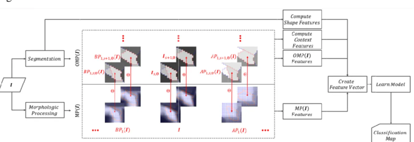
An overview of the approach for computation of OMPs and subsequent processing is given in Fig. 1.

Fig. 1. Overview of the OMP approach. morphological profiles

procedure. The obtained image objects are used to aggregate corresponding features

describing the individual image objects learning a supervised classification model.

In parallel to the computation of conventional MPs to model image objects. Since it may often be necessary with various sizes, a multi

is partitioned with an arbitrary segmentation algorithm at a generic segmentation level objects

unambiguous hierarchy of levels can be established by implementing the following constraint: operations are considered.

completing MOs, transform and black top

They are denoted with follows:

where is the first operation with a SE of size part of the MP is defined as follows:

is the second operation with a SE of size by collation of both sequences:

( ) = [

This way, a feature vector with a dimensionality of ( ) correspond to

AGGREGATED

An overview of the approach for computation of OMPs and subsequent processing is given in

Overview of the OMP approach. morphological profiles

procedure. The obtained image objects are used to aggregate corresponding features

describing the individual image objects learning a supervised classification model.

In parallel to the computation of conventional MPs to model image objects. Since it may often be necessary with various sizes, a multi

is partitioned with an arbitrary segmentation algorithm at a generic segmentation level objects ( = 1,2

unambiguous hierarchy of levels can be established by implementing the following constraint: considered. However, here, we use the term to describe the

, such as erosion and dilation, opening and closing, or black top-hat transform

They are denoted with

is the first operation with a SE of size part of the MP is defined as follows:

[ ( ),

a feature vector with a dimensionality of

correspond to , which is located in the center of the profile

GGREGATED MORPHOLOGICAL

Overview of the OMP approach.

morphological profiles ( ) are obtained from

procedure. The obtained image objects are used to aggregate

corresponding features ( ( )) can be employed in conjunction with spatial context and shape describing the individual image objects

learning a supervised classification model.

In parallel to the computation of conventional MPs to model image objects. Since it may often be necessary

with various sizes, a multi-level, hierarchical segmentation procedure can be

is partitioned with an arbitrary segmentation algorithm at a generic segmentation level

2, … , ). If more than a single segmentation level is considered, an unambiguous hierarchy of levels can be established by implementing the following constraint:

However, here, we use the term to describe the erosion and dilation, opening and closing, or transform applied in a sequential manner to

( ) and

( ) =

is the first operation with a SE of size part of the MP is defined as follows:

( ) =

( ), … ,

a feature vector with a dimensionality of

which is located in the center of the profile

ORPHOLOGICAL

Overview of the OMP approach. The original image are obtained from

procedure. The obtained image objects are used to aggregate

) can be employed in conjunction with spatial context and shape describing the individual image objects and their

learning a supervised classification model.

In parallel to the computation of conventional MPs to model image objects. Since it may often be necessary

level, hierarchical segmentation procedure can be

) If more than a single segmentation level is considered, an unambiguous hierarchy of levels can be established by implementing the following constraint:

However, here, we use the term to describe the erosion and dilation, opening and closing, or

applied in a sequential manner to ( ). As such,

( ), ∀ ∈ is the first operation with a SE of size

( ), ∀ ∈ is the second operation with a SE of size

( ), , a feature vector with a dimensionality of

which is located in the center of the profile

ORPHOLOGICAL OPERATORS AND

The original image are obtained from . In addition, procedure. The obtained image objects are used to aggregate

can be employed in conjunction with spatial context and shape and their spatial context

In parallel to the computation of conventional MPs, to model image objects. Since it may often be necessary

If more than a single segmentation level is considered, an unambiguous hierarchy of levels can be established by implementing the following constraint:

applied in a sequential manner to As such, the first part of the

∈ [0, ] is the first operation with a SE of size from 0 to

[0, ] is the second operation with a SE of size from 0 to

( ), … ,

a feature vector with a dimensionality of 2 + 1 is created. Naturally, which is located in the center of the profile

PERATORS AND OBJECT

The original image is processed in two ways. First, conventional In addition, is subject to a multi

procedure. The obtained image objects are used to aggregate ( ) with an aggr

can be employed in conjunction with spatial context and shape

spatial context. Finally, the created feature vector is used for

, is subject to a segmentation procedure to model image objects. Since it may often be necessary to account

applied in a sequential manner to with varying size of the first part of the

from 0 to . Consequently, the

from 0 to . The actual

( ),

is created. Naturally, which is located in the center of the profile.

BJECT-BASED

is processed in two ways. First, conventional is subject to a multi

) with an aggregation function can be employed in conjunction with spatial context and shape

. Finally, the created feature vector is used for

is subject to a segmentation procedure to account for objects in the image level, hierarchical segmentation procedure can be

If more than a single segmentation level is considered, an unambiguous hierarchy of levels can be established by implementing the following constraint: However, here, we use the term to describe the concatenation of

erosion and dilation, opening and closing, or white top with varying size of the first part of the MP is defined as

Consequently, the

actual MP is obtained

( )]. is created. Naturally,

ASED PROFILES

is processed in two ways. First, conventional is subject to a multi-level segmentation

egation function

can be employed in conjunction with spatial context and shape-related features . Finally, the created feature vector is used for

is subject to a segmentation procedure for objects in the image level, hierarchical segmentation procedure can be adopted

5

concatenation of white top-hat with varying size of is defined as

(7) Consequently, the second

(8) MP is obtained

(9) ( ) and

ROFILES

is processed in two ways. First, conventional level segmentation egation function . The related features . Finally, the created feature vector is used for

is subject to a segmentation procedure for objects in the image adopted [22]. is partitioned with an arbitrary segmentation algorithm at a generic segmentation level in

(6)

6

= .

⊆ +1

(10)

This relation ensures that an object at segmentation level must be included in only one object at level + 1 [24] and thus allows building a consistent profile. Thereby, a defined number of consecutive segmentations can be carried out to establish an exhaustive set of hierarchical image levels Ψ ∈ [ , s + 1, … , ], < . Then, a new grey-level value is assigned to an object based on the grey-level value of corresponding pixels using an arbitrary aggregation function, which is denoted with Θ. In this paper, we deploy three statistical measures of central tendency, namely, mean ( ̅), mode ( ), and median ( ). It can be noted that e.g., statistical measures of spread (variance, or standard deviation) can be considered less relevant in this context since morphological operators impose prior homogeneity constrains on the transformed image.

In concordance with the definition of a MP, we consider the first part of an OMP as follows:

, , ( ) = ( ) ( ), ∀ ∈ [0, ] (11)

where is the first operation with a SE of size from 0 to , ( ) represents the set of hierarchical segmentations obtained from the non-transformed image , and is the aggregation function. Analogously, the second part of the OMP is defined as follows:

, , ( ) = ( ) ( ), ∀ ∈ [0, ] (12)

where is the second operation with a SE of size from 0 to . The actual OMP is obtained by collation of both sequences:

( )

= _{, ,} ( ), _{, ,} ( ), … , _{, ,} ( ), _, , _{, ,} ( ), … , _{, ,} ( ), _{, ,} ( )

(13)

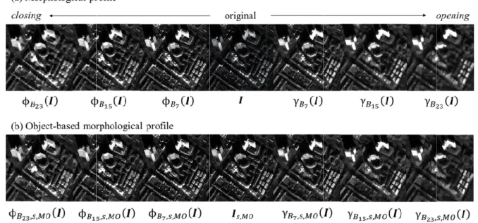
Consequently, the feature vector of an OMP corresponds to a dimensionality of (2 + 1) ∗ . An OMP based on a single segmentation level is exemplified in Appendix A [Fig. 6]. In this example ( ) represents a closing and ( ) an opening.

A favorable property of OMPs and their inherent processing techniques is the ability to derive further features based on generated discrete image regions (i.e., objects). In this paper, we consider two groups of features. The first group comprises shape-related features, whereas the second group contains contextual features describing (topological) neighborhood relationships. The shape-related features are retrieved to account for distinctively diverse geometric properties of LULC objects. For instance, in urban environments natural objects such as vegetation feature frequently a non-rectangular shape, whereas man-made objects such as buildings feature rectangular shapes, which can be employed for learning a discriminative classification model. A comprehensive number of measures can be found in literature to encode such relations. In this manuscript, we characterize the extent of modelled objects by computing area and perimeter. In addition, widely deployed measures that provide an approximate comparison of an object’s shape with 2-D geometrical forms such as rectangle, circle or ellipse are included. Here, five complement measures are used, namely

(7)

rectangular fit explanations and context with respect to an objects values as follows: where

between two objects, which serves as weight. Thereby, the range of feature values correspond

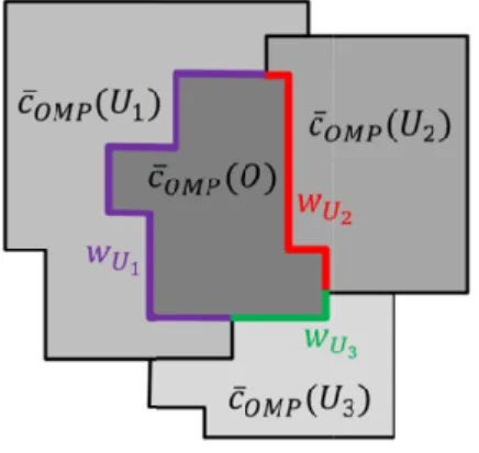
Fig. 2. Exemplified scheme for the computation of contextual features. The individual grey

̅ ( )

common border

It can be noted that brighter or darker ad difference with respect to

motivated by the circumstance that

other such as elevated objects and corresponding shadow areas. can be

classification model. IV.

The experimental analysis was carried out by classifying two panchromatic image

WorldView

rectangular fit, roundness

explanations and formulae can be found in context the objects are embedded in,

with respect to an (Fig. 2). We as follows:

is an adjacent neighbor object of

between two objects, which serves as weight. Thereby, the range of feature values corresponds to

= max

̅

Exemplified scheme for the computation of contextual features. The individual grey of an object is compared to the grey

common border serves as weight for calculating the weighted mean difference of grey

It can be noted that brighter or darker ad difference with respect to

motivated by the circumstance that

other such as elevated objects and corresponding shadow areas. stacked to a

classification model.

DATA SETS AND EXPERIM

The experimental analysis was carried out by classifying two panchromatic image

WorldView-II satellite

roundness,

formulae can be found in the objects are embedded in,

OMP is compared to the affiliated We compute the

̅ _{( ) =}

between two objects, which serves as weight. Thereby, the range of feature values

max |( ̅

̅ _{( ) ∈ {ℝ}

Exemplified scheme for the computation of contextual features. The individual grey of an object is compared to the grey

serves as weight for calculating the weighted mean difference of grey

It can be noted that this scheme allows also considering e.g., only the grey brighter or darker adjacent neighbor object

difference with respect to . Overall, motivated by the circumstance that

other such as elevated objects and corresponding shadow areas. to a joint

classification model.

ATA SETS AND EXPERIM

The experimental analysis was carried out by classifying two panchromatic image. This image

satellite sensor on

, elliptic fit formulae can be found in the objects are embedded in, an individual

is compared to the affiliated compute the weighted

) = 1

∈

|( ̅ ( ) − ̅ {ℝ|−

Exemplified scheme for the computation of contextual features. The individual grey of an object is compared to the

grey-serves as weight for calculating the weighted mean difference of grey

this scheme allows also considering e.g., only the grey jacent neighbor object

. Overall, a

motivated by the circumstance that thematic classes can occur in other such as elevated objects and corresponding shadow areas.

feature vector, which is subsequently fed to a supervised

ATA SETS AND EXPERIMENTAL SETUP

The experimental analysis was carried out by classifying two image was acquired

sensor on 31st January

elliptic fit, compactness

formulae can be found in e.g., [ an individual is compared to the affiliated

weighted mean difference

̅ ( )

is an adjacent neighbor object of , and

̅ ( ) − ̅

̅ ( )|, |

≤ ̅ (

Exemplified scheme for the computation of contextual features. The individual grey -level values

serves as weight for calculating the weighted mean difference of grey

this scheme allows also considering e.g., only the grey jacent neighbor objects of and quantify the affiliated

a quantification of contextual relations is thematic classes can occur in

other such as elevated objects and corresponding shadow areas.

ENTAL SETUP

The experimental analysis was carried out by classifying two

acquired over the city of Cologne, Germany, January 2014 with a geometric resolution of 0.5 m.

compactness, and

e.g., [31]-[33]). gray-level value is compared to the affiliated grey-level value

mean difference

( ) − ̅ ( )

, and is the length of the common border between two objects, which serves as weight. Thereby, the range of feature values

̅ ( )|, …

) |( ̅ ( ) −

( ) ≤

Exemplified scheme for the computation of contextual features. The individual grey

level values ̅ ( ) of neighbor objects. The length of a serves as weight for calculating the weighted mean difference of grey

this scheme allows also considering e.g., only the grey and quantify the affiliated quantification of contextual relations is thematic classes can occur in

other such as elevated objects and corresponding shadow areas.

The experimental analysis was carried out by classifying two

over the city of Cologne, Germany, with a geometric resolution of 0.5 m.

, and shape index

To characterize the level value ̅

level value ̅ mean difference ̅ between

( ) ,

is the length of the common border between two objects, which serves as weight. Thereby, the range of feature values

… ,

( ) − ̅ ( )

}.

Exemplified scheme for the computation of contextual features. The individual grey

of neighbor objects. The length of a serves as weight for calculating the weighted mean difference of grey

this scheme allows also considering e.g., only the grey and quantify the affiliated quantification of contextual relations is

thematic classes can occur in (spatial) dependence of each other such as elevated objects and corresponding shadow areas. Finally, individual features feature vector, which is subsequently fed to a supervised

The experimental analysis was carried out by classifying two test areas

over the city of Cologne, Germany, with a geometric resolution of 0.5 m.

shape index (corresponding

To characterize the ( ) of an object ̅ ( ) of neighbor between the grey

( )| ,

Exemplified scheme for the computation of contextual features. The individual grey-level value of neighbor objects. The length of a serves as weight for calculating the weighted mean difference of grey-level values.

this scheme allows also considering e.g., only the grey-level values of and quantify the affiliated mean grey quantification of contextual relations is primarily

dependence of each , individual features feature vector, which is subsequently fed to a supervised

taken from a VHR over the city of Cologne, Germany,

with a geometric resolution of 0.5 m.

7

(corresponding To characterize the (spatial) object neighbor he grey-level

(14)

(15)

level value of neighbor objects. The length of a

level values of grey-level primarily dependence of each , individual features feature vector, which is subsequently fed to a supervised

taken from a VHR over the city of Cologne, Germany, by the with a geometric resolution of 0.5 m. The

(8)

8

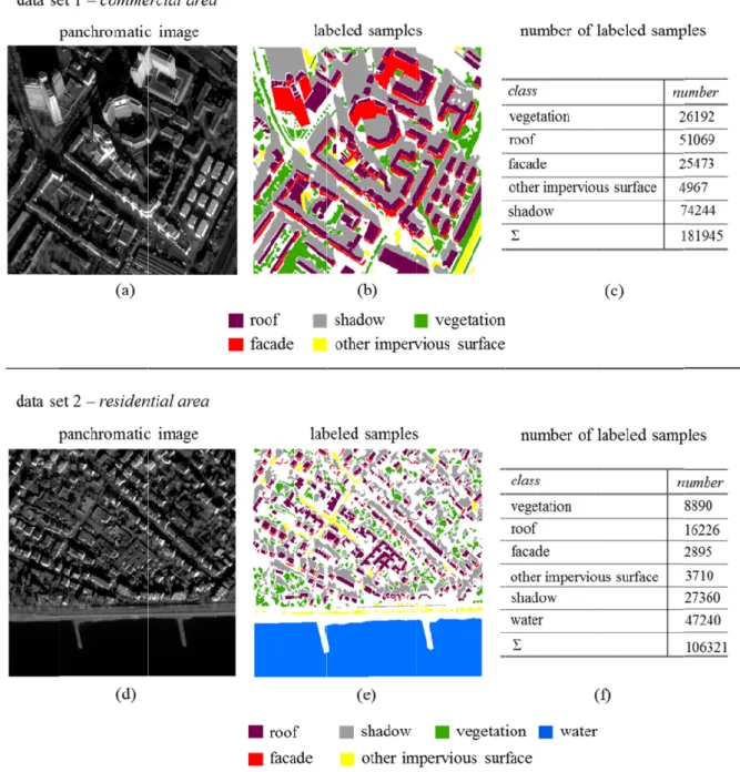
first data set is made up by 1000 × 1000 pixels and shows an urban area of Cologne, which is dominated by buildings of commercial use (Fig. 3(a); referred to as “data set 1 – commercial

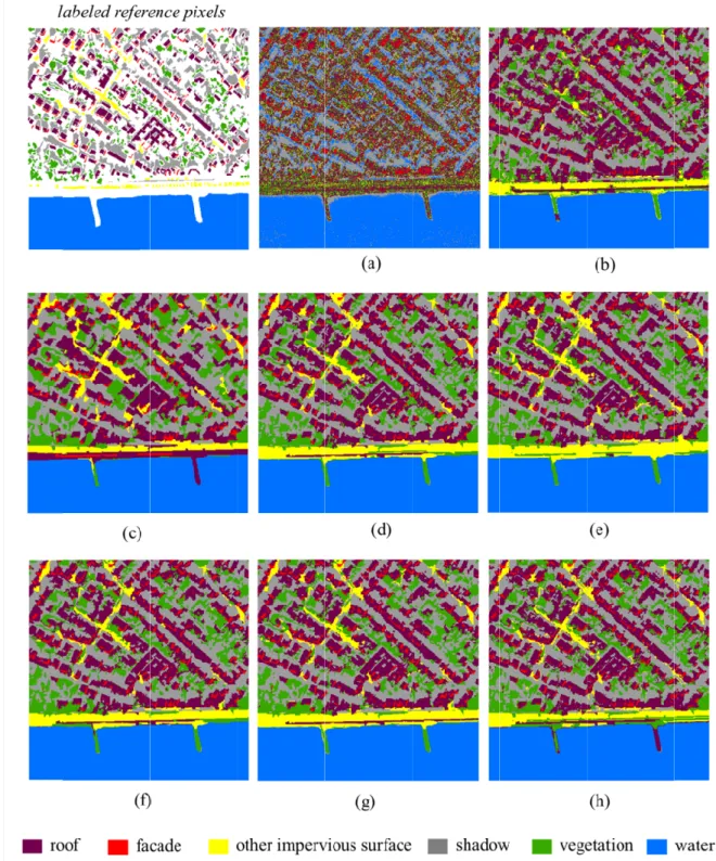
area”). The second data set comprises 902 × 908 pixels and represents an area of residential buildings next to the river Rhine (Fig. 3(d); referred to as “data set 2 – residential area”). Both image subsets feature a complex composition of urban land cover. Thereby, shadow areas can be observed primarily adjacent to buildings. In addition, the imagery represents an off-nadir acquisition. As such, facades of individual buildings can be identified in the direction of the sensor view. The pixels of the first image were grouped in five relevant thematic classes, namely “roof”, “facade”, “shadow”, “vegetation”, and “other impervious surface”. The latter class comprises non-penetrable surfaces other than building-related ones such as roads or parking lots, which feature similar spectral characteristics. Data set 2 additionally features the thematic class “water”. The thematic classes of pixels were determined based on photo-interpretation analysis under consideration of additional aerial imagery and cadastral maps. Varying configurations of corresponding labeled samples of data set 1 and 2 [Fig. 3(b-c) and (e-f)] were used for learning the models. In particular, five percent of all available labeled samples were drawn randomly in a stratified manner (i.e., in correspondence to the a priori probabilities of the classes) from the training data pool of the respective data set for ten different realizations. Thereby, generalization capabilities of the learned models are estimated based on a fivefold cross-validation procedure.

(9)

Fig. 3. Experimental data. (a), ( Germany

For both images, we obtained the considered closing, opening by top

increasing size (i.e., 7, 11, 15, 19, 23). can yield favorable results

benchmark vector in this work (denoted as features 31 dimensions.

Regarding the

segmentation algorithm for partition of in the software environment eCognition [ settings [e.g.,

rather than on gray

due to the fact that manmade structures such as buildings and other elements of urban

Experimental data. (a), (

Germany with available labeled samples (b

For both images, we obtained the considered closing, opening by top

increasing size (i.e., 7, 11, 15, 19, 23). can yield favorable results

Regarding the

segmentation algorithm for partition of in the software environment eCognition [ settings [e.g., [35], [36]

rather than on gray

due to the fact that manmade structures such as buildings and other elements of urban

Experimental data. (a), (d) data sets from WorldView with available labeled samples (b

For both images, we obtained the considered closing, opening by top-hat, and closing by top increasing size (i.e., 7, 11, 15, 19, 23).

can yield favorable results [3

Regarding the computation of segmentation algorithm for partition of in the software environment eCognition [

[35], [36]). In the experiments, we put more emphasis on shape heterogeneity rather than on gray-value heterogeneity with respect to the segmentation algorithm. This is due to the fact that manmade structures such as buildings and other elements of urban

) data sets from WorldView with available labeled samples (b-c; e-f)

For both images, we obtained the considered hat, and closing by top

increasing size (i.e., 7, 11, 15, 19, 23). Since previous works show

3], the obtained sequences were stacked and considered as the benchmark vector in this work (denoted as

computation of segmentation algorithm for partition of in the software environment eCognition [

). In the experiments, we put more emphasis on shape heterogeneity value heterogeneity with respect to the segmentation algorithm. This is due to the fact that manmade structures such as buildings and other elements of urban

) data sets from WorldView f).

For both images, we obtained the considered

hat, and closing by top-hat) based on a square Since previous works show

the obtained sequences were stacked and considered as the benchmark vector in this work (denoted as (

computation of OMPs, we

(i.e., fractal net evolution approach as implemented in the software environment eCognition [34], since it showed viable results in comparable ). In the experiments, we put more emphasis on shape heterogeneity value heterogeneity with respect to the segmentation algorithm. This is due to the fact that manmade structures such as buildings and other elements of urban

) data sets from WorldView-II imagery acquired over the city of Cologne

For both images, we obtained the considered MOs (i.e., erosion, dilation, o hat) based on a square

Since previous works show

the obtained sequences were stacked and considered as the

( ) ).

, we deploy

(i.e., fractal net evolution approach as implemented ], since it showed viable results in comparable ). In the experiments, we put more emphasis on shape heterogeneity value heterogeneity with respect to the segmentation algorithm. This is due to the fact that manmade structures such as buildings and other elements of urban

II imagery acquired over the city of Cologne

(i.e., erosion, dilation, o

hat) based on a square-shaped SE with linear Since previous works showed that sets of mixed the obtained sequences were stacked and considered as the

). Consequently, a bottom-up region

(i.e., fractal net evolution approach as implemented ], since it showed viable results in comparable ). In the experiments, we put more emphasis on shape heterogeneity value heterogeneity with respect to the segmentation algorithm. This is due to the fact that manmade structures such as buildings and other elements of urban

II imagery acquired over the city of Cologne

(i.e., erosion, dilation, o

shaped SE with linear d that sets of mixed the obtained sequences were stacked and considered as the

Consequently, ( up

region-(i.e., fractal net evolution approach as implemented ], since it showed viable results in comparable ). In the experiments, we put more emphasis on shape heterogeneity value heterogeneity with respect to the segmentation algorithm. This is due to the fact that manmade structures such as buildings and other elements of urban

9 II imagery acquired over the city of Cologne,

(i.e., erosion, dilation, opening, shaped SE with linear d that sets of mixed MOs the obtained sequences were stacked and considered as the

)

-growing (i.e., fractal net evolution approach as implemented ], since it showed viable results in comparable ). In the experiments, we put more emphasis on shape heterogeneity value heterogeneity with respect to the segmentation algorithm. This is due to the fact that manmade structures such as buildings and other elements of urban

(10)

10

environments have distinct shape and size properties, unlike, for example, natural features. Analogously, the weights for heterogeneity of smoothness and compactness were maintained equal (i.e., shape: 0.7, color: 0.5) and kept constant. Three hierarchical segmentation levels were considered for the experiments to account for objects with various sizes in the image. The scale parameters which determine - briefly speaking - the size of the objects, were chosen in a way that 1) at , the majority of real-world objects are represented by several segments (i.e., over-segmentation); 2) at + 1, the majority of real-world objects are represented by a single affiliated segment; and 3) at + 2, the majority of real-world objects are represented in conjunction with other real-world objects by a single segment (i.e., under-segmentation) [37]. In accordance with the experimental setup of e.g., Dalla Murra et al. [14], we deploy a Random Forest (RF) approach [38] for evaluating the capabilities of the different profiles in modeling the characteristics of the respective imagery. This non-parametric classification approach was chosen to account for a considerable redundancy shown by the profiles (primarily induced by the consecutive window sizes and segmentation scales of the same morphological operations), which can be critical for the estimation of statistics in parametric approaches [14]. RF represents a decision-tree-based ensemble learning method for classification and regression. Such methods build a prediction model by utilizing the strength of a collection of simple base models. To this purpose, RF grows multiple decision trees on random subsets of the training data. The high variance among individual trees, letting each tree vote for the class assignment, and determining the respective class according to the majority of the votes, allows the accurate and robust classification of unlabeled samples, even when many noisy variables are existent [38], [39]. The hyperparameters that need to be determined for generating a RF model consist of the number of classification trees to be grown n_tree, and the number of features m_try used at each node. To provide a reliable error estimate and maintaining the computation times in a reasonable range, we chose a n_tree value of 500. This is in a good agreement with the RF parameter study performed by Genuer et al. [40]. According to Breiman [38], a value for m_try= p, with p denoting the number of input

features, yields near optimum classification results. Thus, this heuristic was used to determine

m_try. To impose ceteris paribus-near conditions for comparison of the computed features a wrapper-based feature selection [41] was carried out to identify feature sets from the complete pool of available features, which allow for obtaining the best accuracies given the aforementioned experimental setup. Wrapper methods evaluate features by using accuracy estimates provided by the actual classification algorithm (here RF), which is deployed subsequent to feature selection. Thus, the classifier is trained and accuracy estimation is performed for each iteration of the evaluation process. Thereby, the respective models with the highest Kappa statistics (κ) – as primal measure for accuracy – were further considered. Such as strategy is very expensive from a computational point of view, however, it ensures most favorable model accuracy possible for a feature set, what is desirable in this comparative evaluation of features.

Thematic accuracies of the obtained maps (which are presented in Tables I and II) were assessed by computing global accuracy measures. We considered the weighted harmonic mean F of the F-measures (weighted by the cardinals of the thematic classes [42]), the overall accuracy (OA), and the κ statistic based on the selected reference pixels (definition of those measures can be found in e.g., [43], [44]). Since overall accuracies of some models feature

(11)

11

comparable levels, the statistical significance of the classification maps was additionally evaluated with the McNemar’s test [43]. The test compares the classification outcomes for related samples (i.e., the number of miss-classified samples by the first model but not by the second model and the number of miss-classified samples by the second model but not by the first model) by assessing the standardized normal test statistic Z for two thematic maps. The

null hypothesis (i.e., the models feature the same error) can be rejected for an interval of significance α= 5%,if |Z|>1.96.The results of this test are indicated in Tables I and II with

the sign “*” when the accuracy of a model is higher and significantly different from the benchmark model (i.e., obtained with ( ) ).

V. EXPERIMENTAL RESULTS AND DISCUSSION

To understand the role of the different groups of features on the classification accuracy, systematic configurations of features were compiled and deployed for classification. Thereby, the different configurations of features were fed to the wrapper-based feature selection scheme described above to eventually prune irrelevant features and ensure most favorable model accuracy possible.

A. Data set 1 – commercial area

The results of this analysis for the data set of the commercial area are documented in Table I in terms of accuracy measures. Selected results are also visualized in Fig. 4. Generally, the results in Table I are differentiated according to the pixel and object-based approaches and with respect to the latter in dependence of the deployed aggregation function.

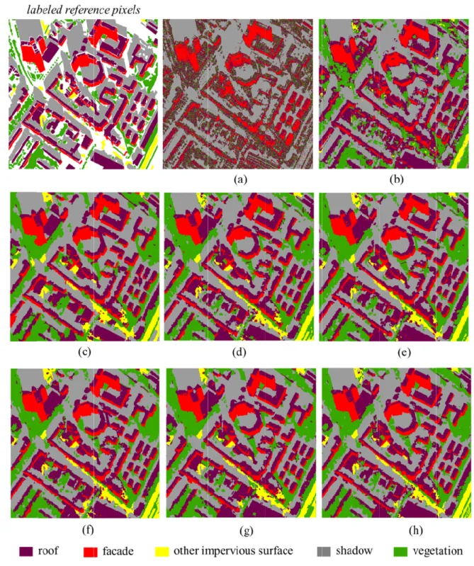
First of all, it can be noticed that the model based on the individual pixels of the panchromatic band does not feature viable accuracies and the affiliated classification map is not spatially consistent at all [Fig. 4(a)]. Instead, the usage of ( ) allows for obtaining a considerably improved level of accuracy and a classification map with definite spatial consistency [Fig. 4(b)]. Regarding the deployment of OBIA techniques, notably, a significant improvement in terms of accuracies can be achieved in this example already with respect to ( ) , when using the object-based representation of the non-transformed image for model learning (i.e., an average increase of more than 7% in terms of κ statistic can be observed independent of the chosen aggregation function). As can be seen from [Fig. 4(c)], spatial assemblages of classes are less fragmented compared to the previous result, however, overgeneralization also occurs. The learning of models based on ( ) provides solutions with a further substantial increase of accuracy (i.e., an average increase of more than 4% and 12% in terms of κ statistic can be observed with respect to the object-based representation of the non-transformed image and ( ) , respectively, independent of the chosen aggregation function). Thereby, the affiliated classification map [Fig. 4(d)] internalizes two favorable aspects, as the solution is clearly less fragmented than

(12)

12 TABLE I

STUDY AREA 1(COMMERCIAL AREA):CLASSIFICATION ACCURACIES OBTAINED WITH DIFFERENT FEATURE VECTORS

REPORTED AS MEAN AND STANDARD DEVIATION (IN BRACKETS) FROM TEN REALIZATIONS WITH A VARYING

CONFIGURATION OF LABELED SAMPLES.“*”=SIGNIFICANT DIFFERENCE FOR AN INTERVAL OF SIGNIFICANCE OF Α =5%

FROM THE BENCHMARK FEATURE VECTOR (I.E., ( ) ) AS EVALUATED WITH MCNEMAR’S TEST AND

CORRESPONDING NUMERICAL VALUES OF MEAN AND STANDARD DEVIATION.RESULTS OBTAINED FOR THE CATEGORIES

“PIXEL-BASED” AND “OBJECT-BASED - MEAN”ARE ALSO VISUALIZED IN FIGURE 4

feature vector accuracy measures

McNemar’s test F (%) OA (%) κ (%) pixel-based I 42.31 (±4.55) 66.86 (±0.21) 52.92 (±0.07) ( ) 84.96 (±0.29) 86.09 (±0.21) 80.36 (±0.36) object-based ̶ mean , ̅ 91.80 (±0.18) 91.86 (±0.18) 88.62 (±0.29) *, 19.84 (±0.04) ( )̅ 94.78 (±0.08) 94.80 (±0.07) 92.72 (±0.12) *, 27.03 (±0.51) ( )̅ , 94.87 (±0.07) 94.88 (±0.08) 92.84 (±0.09) *, 27.19 (±0.63) ( )̅ , ( ) ̅ 94.78 (±0.08) 94.83 (±0.06) 92.74 (±0.11) *, 27.08 (±0.56) ( )̅ , , ( )̅ 94.93 (±0.03) 94.94 (±0.04) 92.94 (±0.04) *, 27.20 (±0.62) ( )̅ , , ( )̅ , ( ) 94.97 (±0.02) 95.02 (±0.03) 93.01 (±0.02) *, 27.29 (±0.69) object-based ̶ mode , 90.77 (±0.04) 90.91 (±0.06) 87.41 (±0.12) *, 17.44 (±0.69) ( ) 94.87 (±0.17) 94.89 (±0.15) 92.85 (±0.24) *, 27.39 (±0.24) ( ) , 94.99 (±0.05) 95.01 (±0.04) 93.01 (±0.08) *, 27.55 (±0.39) ( ) , ( ) 94.87 (±0.17) 94.89 (±0.15) 92.85 (±0.24) *, 27.44 (±0.28) ( ) , , ( ) 95.04 (±0.12) 95.04 (±0.09) 93.02 (±0.07) *, 27.58 (±0.41) ( ) , , ( ) , ( ) 95.13 (±0.13) 95.05 (±0.06) 93.08 (±0.05) *, 27.62 (±0.47) object-based ̶ median , 91.17 (±0.05) 91.29 (±0.05) 87.79 (±0.03) *, 19.30 (±0.16) ( ) 94.71 (±0.03) 94.74 (±0.02) 92.63 (±0.04) *, 26.86 (±0.21) ( ) , 94.84 (±0.03) 94.89 (±0.05) 92.76 (±0.02) *, 27.65 (±0.09) ( ) , ( ) 94.72 (±0.06) 94.77 (±0.04) 92.63 (±0.04) *, 27.40 (±0.08) ( ) , , ( ) 94.88 (±0.09) 95.02 (±0.02) 92.90 (±0.09) *, 27.74 (±0.09) ( ) , , ( ) , ( ) 94.89 (±0.04) 95.04 (±0.03) 93.05 (±0.05) *, 27.82 (±0.04)

The encoding of shape and context-related properties enables an additional slight increase of model accuracies compared to ( ) [Fig. 4(e)-(g)]. Thereby, the shape-related features are more valuable in this example than the context-related ones, since the increase of accuracy is consistently a little higher. A joint consideration of both groups of features allows for obtaining further increased accuracies. This indicates that both groups of features can

(13)

13

encode additional discriminative information compared to the solely application of both MPs or OMPs. Lastly, the creation of feature vectors containing all features allowed for further slight improvements and ensures the highest accuracies observed during all runs.

A clear recommendation regarding the most favorable aggregation function cannot be drawn from this example. This is evident since the most favorable feature vectors of different categories are attributed to different aggregation functions. However, the results do not vary greatly between the different aggregation functions and the overall accuracy pattern is consistent - independent of the chosen aggregation function. Overall, feature vectors based on OMPs reveal more favorable results than models obtained with MPs, what demonstrates the viability of this concept.

(14)

Fig. 4. Classification results obtained with different feature vectors

transformed panchromatic imagery; (b)

, ̅, (

( ) _̅ ( ) _̅ ( ) _̅ consideration of

Classification results obtained with different feature vectors

, (object-based non

̅ ; (e)

̅ under additional consideration of context features

̅ under additional consideration of both shape and context features; (h)

consideration of (

based non-transformed panchromatic imagery ; (e) ( ) _̅

under additional consideration of context features under additional consideration of both shape and context features; (h)

) .

transformed panchromatic imagery

̅ under additional consideration of shape features; (f)

under additional consideration of context features under additional consideration of both shape and context features; (h)

under additional consideration of shape features; (f) under additional consideration of context features

under additional consideration of both shape and context features; (h) Classification results obtained with different feature vectors for the commercial area

under additional consideration of both shape and context features; (h) commercial area

transformed panchromatic imagery; (b) (

based on

under additional consideration of both shape and context features; (h) same as (g) but add commercial area. (a) pixel-based non

) ;

based on mean)

under additional consideration of shape features; (f) under additional consideration of context features; (g)

same as (g) but add

14 based non-(c) mean); (d) under additional consideration of shape features; (f)

; (g)

(15)

15 B. Data set 2 – residential area

The classification accuracies for the data set of the residential area are documented in Table II and the application of selected models can be found in Fig. 5. In accordance with the results from data set 1, the information of the single panchromatic image cannot reliably partition the pixels in thematic classes [Fig. 5(a)]. Again, the use of MPs enables a steep increase of accuracy measures (e.g., from 61% to 93% in terms of κ statistic) and a stable classification map with respect to its spatial consistency [Fig. 5(b)]. An improvement can be obtained also for this example when relying on the object-based representation of the non-transformed image for model learning [Fig 5(c)] compared to the outcomes achieved with the single panchromatic image. However, in contrast to the previous example, this model features lower accuracies compared to ( ) . Instead, the postulated OMPs exceed the accuracy of the benchmark vector considerably again (i.e., an average increase of more than 4% in terms of κ statistic can be observed independent of the chosen aggregation function), although the levels of model accuracies are already very high. Moreover, as for the previous data set, the considered shape and context-related features allow for a further increase of model performance. In accordance, the highest accuracies can be retrieved based on all available features.

(16)

16 TABLE II

STUDY AREA 2(COMMERCIAL AREA):CLASSIFICATION ACCURACIES OBTAINED WITH DIFFERENT FEATURE VECTORS

REPORTED AS MEAN AND STANDARD DEVIATION (IN BRACKETS) FROM TEN REALIZATIONS WITH A VARYING

CONFIGURATION OF LABELED SAMPLES.“*”=SIGNIFICANT DIFFERENCE FOR AN INTERVAL OF SIGNIFICANCE OF Α =5%

FROM THE BENCHMARK FEATURE VECTOR (I.E., ( ) ) AS EVALUATED WITH MCNEMAR’S TEST AND

CORRESPONDING NUMERICAL VALUES OF MEAN AND STANDARD DEVIATION.RESULTS OBTAINED FOR THE CATEGORIES

“PIXEL-BASED” AND “OBJECT-BASED - MEAN”ARE ALSO VISUALIZED IN FIGURE 4

feature vector accuracy measures

McNemar’s test F (%) OA (%) κ (%) pixel-based I 61.25 (±0.18) 72.92 (±0.06) 60.90 (±0.23) ( ) 93.95 (±0.02) 94.90 (±0.04) 92.77 (±0.01) object-based ̶ mean , ̅ 94.69 (±0.04) 94.64 (±0.03) 92.37 (±0.05) - ( )̅ 97.71 (±0.12) 97.77 (±0.12) 96.85 (±0.16) *, 10.79 (±0.20) ( )̅ , 97.82 (±0.03) 97.89 (±0.05) 97.01 (±0.05) *, 11.17 (±0.10) ( )̅ , ( ) ̅ 97.86 (±0.04) 97.92 (±0.05) 97.06 (±0.05) *, 11.17 (±0.04) ( )̅ , , ( )̅ 98.00 (±0.10) 98.05 (±0.08) 97.25 (±0.14) *, 11.40 (±0.27) ( )̅ , , ( )̅ , ( ) 98.36 (±0.01) 98.39 (±0.01) 97.43 (±0.32) *, 13.28 (±0.08) object-based ̶ mode , 93.29 (±0.44) 93.91 (±0.33) 91.37 (±0.52) - ( ) 97.89 (±0.04) 97.95 (±0.04) 97.10 (±0.07) *, 10.71 (±0.93) ( ) , 97.94 (±0.05) 97.99 (±0.03) 97.16 (±0.01) *, 10.89 (±0.75) ( ) , ( ) 97.92 (±0.02) 97.98 (±0.01) 97.14 (±0.03) *, 10.89 (±0.75) ( ) , , ( ) 97.94 (±0.01) 97.99 (±0.02) 97.16 (±0.01) *, 10.91 (±0.73) ( ) , , ( ) , ( ) 98.37 (±0.09) 98.40 (±0.09) 97.74 (±0.14) *, 12.60 (±0.88) object-based ̶ median , 93.43 (±0.10) 93.98 (±0.05) 91.46 (±0.05) - ( ) 97.74 (±0.13) 97.82 (±0.13) 96.92 (±0.16) *, 10.49 (±0.03) ( ) , 97.88 (±0.06) 97.94 (±0.07) 97.09 (±0.08) *, 10.96 (±0.26) ( ) , ( ) 98.01 (±0.14) 98.07 (±0.12) 97.27 (±0.19) *, 11.26 (±0.81) ( ) , , ( ) 98.06 (±0.08) 98.11 (±0.08) 97.32 (±0.13) *, 11.30 (±0.77) ( ) , , ( ) , ( ) 98.26 (±0.08) 98.32 (±0.08) 97.62 (±0.13) *, 12.29 (±0.86)

As can be seen from the visualization of the OMP-based models [Fig 5(d)-(h)], which all exceed the accuracy of the baseline vector, the obtained maps are not only spatially less fragmented again but also some thematic classes are in general extracted way more reliably. This can be prominently observed for the thematic class “other impervious surface”, which

(17)

can be

mean recall rate of the models based on

mean recall rate of the models based on the OMP universal superiority with respect to

however, the overall accuracy patterns is consistent. Finally affiliated feature vectors enabled learning of models accuracy compared to standard

Fig. 5. Classification results obtained with different feature vectors for the

, ̅, (

retrieved in this example

Classification results obtained with different feature vectors for the

, (object-based non

in this example

based non-transformed panchromatic imagery based on mean); (d)

in this example with a significantly decreased er mean recall rate of the models based on

mean recall rate of the models based on the OMP universal superiority with respect to one particular

however, the overall accuracy patterns is consistent. Finally affiliated feature vectors enabled learning of models accuracy compared to standard MPs again.

transformed panchromatic imagery based on mean); (d)

with a significantly decreased er mean recall rate of the models based on ( )

mean recall rate of the models based on the OMP-processing corresponds to

one particular aggregation function cannot be observed, however, the overall accuracy patterns is consistent. Finally

affiliated feature vectors enabled learning of models MPs again.

with a significantly decreased er

is 0.552 for this class, whereas the processing corresponds to

aggregation function cannot be observed, however, the overall accuracy patterns is consistent. Finally, it can be noted that

affiliated feature vectors enabled learning of models which exhibit

Classification results obtained with different feature vectors for the residential area

with a significantly decreased error of

is 0.552 for this class, whereas the processing corresponds to

aggregation function cannot be observed, it can be noted that

which exhibit a significant increased

residential area

transformed panchromatic imagery; (b) (

or of omission (i.e., is 0.552 for this class, whereas the processing corresponds to 0.882). A

aggregation function cannot be observed, it can be noted that OMPs and

a significant increased

residential area. (a) pixel-based non

) ;

transformed panchromatic imagery based on mean); (d) 17

(i.e., the is 0.552 for this class, whereas the Again, a aggregation function cannot be observed, OMPs and a significant increased

based non-(c) transformed panchromatic imagery based on mean); (d)

(18)

18 ( ) ̅ ; (e) ( ) ̅ under additional consideration of shape features; (f)

( ) _̅ under additional consideration of context features; (g)

( ) ̅ under additional consideration of both shape and context features; (h) same as (g) but additional

consideration of ( ) .

VI. CONCLUSIONS AND OUTLOOK

In this paper, the concept of object-based morphological profiles was introduced for classification of very high spatial resolution remote sensing images. A formal definition of OMPs and experimental evaluation were provided. OMPs are intended to allow for a very flexible and exhaustive characterization of various objects in an image with respect to morphologic operators. As such, they allow for a multi-level decomposition of an image considering also shape-related, topological, and hierarchical properties of affiliated image objects (i.e., discrete image regions). Thereby, this work can be attributed to, and extends the methodological canon of object-based image analysis techniques, which is found to represent an emerging paradigm in the context of remote sensing and geographic information science [1].

The proposed technique was applied to two portions of very high spatial resolution panchromatic imagery acquired by the WorldView-II sensor. The imagery was classified according to relevant urban LULC classes within random forest architecture. Thereby, a comprehensive number of features based on OMPs was computed and employed for classification. In this, various feature sets were compiled to understand the role of the different groups of features that can be retrieved based on OMPs. The results underline the effectiveness of the proposed OMPs, which allow for obtaining a significantly increased classification accuracy of learned models compared to standard MPs, and enhanced spatial consistency of classification maps.

Subsequent works can address the extension of this concept for processing of multi- and hyperspectral imagery. Thereby, the implementation of a proper dimensionality reduction scheme (e.g., principle component analysis) appears imperative to alleviate the computational burden associated with feature selection based on filters and in particular wrapper-based methods for high-dimensional data sets. Moreover, a tailored classification approach based on e.g., a SVM with multi-source composite kernels could provide beneficial joint consideration of the spectral and spatial information. Finally, it would be very interesting to benchmark OMPs in a consistent experimental setup, which allows for stringent comparability, with respect to results obtained by other advanced mathematical morphology-based processing techniques such as attribute profiles.

VII. APPENDIX A

Fig. 6 shows an exemplification of a ( ) and corresponding ( ). The considered MOs opening and closing were obtained with a square-shaped SE. One segmentation level was created for the ( ) and mode was used as aggregation function.