A New Quadratic Binary Harris Hawk Optimization For Feature Selection

(1)

Article

A New Quadratic Binary Harris Hawk Optimization

for Feature Selection

Jingwei Too1,* , Abdul Rahim Abdullah1,* and Norhashimah Mohd Saad2

1 _{Fakulti Kejuruteraan Elektrik, Universiti Teknikal Malaysia Melaka, Hang Tuah Jaya, 76100 Durian Tunggal,} Melaka, Malaysia

2 _{Fakulti Kejuruteraan Elektronik dan Kejuruteraan Komputer, Universiti Teknikal Malaysia Melaka,} Hang Tuah Jaya, 76100 Durian Tunggal, Melaka, Malaysia; [email protected]

* Correspondence: [email protected] (J.T.); [email protected] (A.R.A.); Tel.:+60-178-845-938 (J.T.) Received: 14 September 2019; Accepted: 30 September 2019; Published: 7 October 2019

Abstract:Harris hawk optimization (HHO) is one of the recently proposed metaheuristic algorithms that has proven to be work more effectively in several challenging optimization tasks. However, the original HHO is developed to solve the continuous optimization problems, but not to the problems with binary variables. This paper proposes the binary version of HHO (BHHO) to solve the feature selection problem in classification tasks. The proposed BHHO is equipped with an S-shaped or V-shaped transfer function to convert the continuous variable into a binary one. Moreover, another variant of HHO, namely quadratic binary Harris hawk optimization (QBHHO), is proposed to enhance the performance of BHHO. In this study, twenty-two datasets collected from the UCI machine learning repository are used to validate the performance of proposed algorithms. A comparative study is conducted to compare the effectiveness of QBHHO with other feature selection algorithms such as binary differential evolution (BDE), genetic algorithm (GA), binary multi-verse optimizer (BMVO), binary flower pollination algorithm (BFPA), and binary salp swarm algorithm (BSSA). The experimental results show the superiority of the proposed QBHHO in terms of classification performance, feature size, and fitness values compared to other algorithms.

Keywords: feature selection; binary optimization; classification; Harris hawk optimization; quadratic transfer function

1. Introduction

In recent days, the data representation has become one of the essential factors that can significantly affect the performance of classification models. To date, more and more high dimensional data are gathered from the process of data acquisition, which introduces the curse of dimensionality to the data mining tasks [1]. In addition, the presence of redundant and irrelevant features is another issue that degrades the performance of the system and brings additional computational cost. Therefore, feature selection has become a critical step in the data mining process. The main goal of feature selection is to select the best combination of potential features that offers a better understanding of the classification model. Feature selection not only improves the prediction accuracy but also reduces the dimension of data [2,3].

Generally, feature selection can be categorized into two classes: filter and wrapper. The filter method is simple, and it can obtain the results faster. However, the filter method does not dependent on the learning algorithm, thus resulting in unsatisfactory performance [4,5]. As compared to the filter method, the wrapper method can usually provide higher classification accuracy. The wrapper method includes a machine learning algorithm as part of the evaluation, which enables it to achieve better classification results than the filter method. Thus, wrapper methods have more widely used in feature selection works [6–8].

(2)

Wrapper feature selection is also known as anNP-hard combinatorial optimization problem in which the possible solutions increase exponentially with the number of features. To date, many researchers adopt metaheuristic algorithms (wrapper methods) to tackle the feature selection problem in classification tasks. From the previous works, metaheuristic algorithms were showing excellent performance when dueling with the feature selection problem. For instance, the binary grey wolf optimization (BGWO) was developed to resolve this problem in [9] as a wrapper feature selection method. Additionally, an enhanced version of grey wolf optimizer, namely multi-strategy ensemble grey wolf optimizer (MEGWO) was designed to solve the feature selection problem on real-world applications [10]. The authors proposed the enhanced global best lead strategy, adaptable cooperative strategy, and disperse foraging strategy to boost the performance of GWO. Sindhu et al. [11] introduced an improved sine cosine algorithm (ISCA) that integrated an elitism strategy for feature selection. Jude Hemanth and Anita [12] developed the modified genetic algorithms to evolve the usage of genetic algorithm for tackling the feature selection issue in brain image classification. Moreover, the binary versions of spotted hydra optimizer and multi-verse optimizer were proposed to solve the feature selection problems as the wrapper methods [13,14]. Recently, a chaotic dragonfly algorithm (CDA) was developed for wrapper feature selection [15]

In this paper, we propose the binary version of Harris hawk optimization (HHO) to tackle the feature selection problem in classification tasks. HHO is a recently proposed metaheuristic algorithm in 2019. Generally, HHO mimics the concepts of Harris hawks to explore the prey, surprise pounce, and different attack strategies of hawks in nature. According to the literature, HHO showed superior performance for several benchmark tests compared to other well-established metaheuristic algorithms [16]. Among the competitors, HHO is highly capable of maintaining a well stable balance between exploration (global search) and exploitation (local search), which allows it to score the best properties in optimization tasks. As a bonus, HHO utilizes a series of search strategies in exploitation that enables it to provide a constructive impact on local search. Thus, HHO can be considered as a powerful algorithm for optimization problems. However, HHO is originally designed to solve the continuous optimization problems, which cannot directly apply to binary optimization problems such as feature selection. To the best of our knowledge, there is no binary version of HHO has proposed to solve the feature selection problems in the literature. Moreover, according to the No Free Lunch (NFL) theorem, no universal metaheuristic algorithm was good at solving all the optimization problems [17]. This motivates us to propose a new binary version of HHO in this work.

In this study, we integrate the S-shaped and V-shaped transfer functions into the algorithm to convert the continuous HHO into the binary version (BHHO). Furthermore, we propose another new variant of HHO, namely quadratic binary Harris hawk optimization (QBHHO) for performance enhancement. Unlike BHHO, QBHHO integrates the quadratic transfer function for the conversion. The proposed BHHO and QBHHO algorithms are used to solve the feature selection problems as wrapper methods. Twenty-two datasets collected from UCI machine learning repository are employed to test the performance of proposed algorithms in this work. Moreover, five state-of-the-art methods include binary differential evolution (BDE), genetic algorithm (GA), binary multi-verse optimizer (BMVO), binary flower pollination algorithm (BFPA), and binary salp swarm algorithm (BSSA) are applied to examine the effectiveness of the proposed algorithm in feature selection. The experimental results reveal the superiority of QBHHO not only in the optimal classification performance but also the minimal number of selected features.

The remainder of this paper is organized as follows: Section2introduces the standard Harris hawk optimization (HHO) algorithm. Section3presents the proposed binary Harris hawk optimization (BHHO) algorithms. In Section4, the detailed on the quadratic binary Harris hawk optimization (QBHHO) algorithms is outlined. Section5demonstrates the application of proposed BHHO and QBHHO algorithms for feature selection. Section6discusses the finding of the experiments. Section7 concludes the findings of this research.

(3)

2. Harris Hawk Optimization

Harris hawk optimization (HHO) is a recent metaheuristic algorithm proposed by Heidari and his colleagues in 2019 [16]. HHO mimics the concepts of Harris hawks to explore the prey, surprise pounce, and different attack strategies of Harris hawks in nature. In HHO, the candidate solutions are represented by hawks, while the best solution (nearly optimal solution) is known as prey. The Harris hawks try to track the prey by using their powerful eyes and then perform the surprise pounce to catch the prey detected.

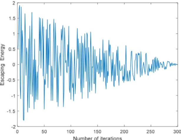
Generally, HHO is modeled into exploitation and exploration phases. The HHO algorithm can be transferred from exploration to exploitation, and then the exploration behavior is changed based on the escaping energy of prey. Mathematically, the escaping energy of prey can be computed as [16]:

E=2E0 1− t T (1) E0=2r−1 (2)

wheretis the current iteration,Tis the maximum number of iterations,E0is the initial energy randomly generated in [−_{1, 1], and}_r_{is a random number in [0, 1]. Figure}₁_{shows an illustration of escaping} energy of prey over 300 iterations. As can be seen, the escaping energy was showing a decreasing trend. When the escaping energy of prey|E|≥_{1, HHO allowed the hawks to search globally on di}ff_erent regions. On the contrary, HHO tended to promote the local search around the neighborhood of the best solutions when the escaping energy of prey|E| <1.

Electronics 2019, 8, x FOR PEER REVIEW 3 of 27

Harris hawk optimization (HHO) is a recent metaheuristic algorithm proposed by Heidari and his colleagues in 2019 [16]. HHO mimics the concepts of Harris hawks to explore the prey, surprise pounce, and different attack strategies of Harris hawks in nature. In HHO, the candidate solutions are represented by hawks, while the best solution (nearly optimal solution) is known as prey. The Harris hawks try to track the prey by using their powerful eyes and then perform the surprise pounce to catch the prey detected.

Generally, HHO is modeled into exploitation and exploration phases. The HHO algorithm can be transferred from exploration to exploitation, and then the exploration behavior is changed based on the escaping energy of prey. Mathematically, the escaping energy of prey can be computed as [16]:

0 2 1 t E E T   =  −    (1) 0 2 1 E = r− (2)

where t is the current iteration, T is the maximum number of iterations, E0is the initial energy randomly generated in [−1, 1], and r is a random number in [0, 1]. Figure 1 shows an illustration of escaping energy of prey over 300 iterations. As can be seen, the escaping energy was showing a decreasing trend. When the escaping energy of prey |E| ≥ 1, HHO allowed the hawks to search globally on different regions. On the contrary, HHO tended to promote the local search around the neighborhood of the best solutions when the escaping energy of prey |E| < 1.

Figure 1. An illustration of escaping energy.

2.1. Exploration Phase

In the exploration phase, the position of the hawk is updated via random location and other hawks as follow [16]: ( )

₍

( )_{( )} 1 _{( )}( )

₎

₍

2 ( )₍ ₎

₎

3 4 2 0.5 1 0.5 k k r m X t r X t r X t q X t X t X t r lb r ub lb q  − − ≥  + = − − + − <  (3)

where X is the position of the hawk, Xkis the position of randomly selected hawk, Xris the position of prey (global best solution in the entire population), t is the current iteration, ub and lb are the upper and lower boundaries of search space, r1, r2, r3, r4, and q are the five independent random numbers in [0, 1]. The Xm is the mean position of the current population of hawks, and it can be computed using Equation (4).

( )

1 1 N m n n X t X t N = =



(4)

where Xn is the n-th hawk in the population, and N is the number of hawks (population size). Figure 1.An illustration of escaping energy.

2.1. Exploration Phase

In the exploration phase, the position of the hawk is updated via random location and other hawks as follow [16]: X(t+1) = ( Xk(t)−r1 Xk(t)−2r2X(t) q≥0.5 (Xr(t)−_Xm(t))−_r₃(lb+r4(ub−lb)) q<0.5 (3) whereXis the position of the hawk,Xkis the position of randomly selected hawk,Xris the position of prey (global best solution in the entire population),tis the current iteration,ubandlbare the upper and lower boundaries of search space,r1,r2,r3,r4, andqare the five independent random numbers in [0, 1]. TheXmis the mean position of the current population of hawks, and it can be computed using Equation (4). Xm(t) = 1 N N X n=1 Xn(t) (4)

(4)

whereXnis then-th hawk in the population, andNis the number of hawks (population size). 2.2. Exploitation Phase

In the exploitation phase, the position of the hawk is updated based on four different situations. This behavior is manipulated based on the escaping energy of prey (E), and the chance of prey in successfully escaping (r<0.5) or not successfully escaping (r≥_{0.5) before surprise bounce.}

2.2.1. Soft Besiege

The soft besiege happens whenr≥_{0.5 and}|_E|≥_{0.5. In this situation, the hawk updates its position} using Equation (5): X(t+1) =∆X(t)−_E JXr(t)−X(t) (5)

whereEis the escaping energy of prey,Xis the position of the hawk,tis the current iteration,∆Xis the difference between the position of the prey and current hawk, andJis the jump strength. The∆XandJ are defined as follows [16]:

∆X(t) =Xr(t)−_X₍_t₎ ₍₆₎

J=2(1−_r₅₎ ₍₇₎

wherer5is a random number in [0, 1] that changes randomly in each iteration. 2.2.2. Hard Besiege

The HHO performs the hard besiege whenr≥_{0.5 and}|_E| <_{0.5. In this situation, the position of} the hawk is updated as follow [16]:

X(t+1) =Xr(t)−_E ∆X(t)

(8)

whereXis the position of the hawk,Xris the position of prey,Eis the escaping energy of prey, and∆X is the difference between the position of the prey and current hawk.

2.2.3. Soft Besiege with Progressive Rapid Dives

The soft besiege with progressive rapid dives is occurred whenr<0.5 and|E|≥_{0.5. The hawk} progressively selects the best possible dive to catch the prey competitively. In this circumstance, the new position of the hawk is generated as follows [16]:

Y=Xr(t)−_E JXr(t)−X(t) (9) Z=Y+α×_Levy₍_D₎ ₍₁₀₎

whereYandZare two newly generated hawks,Eis the escaping energy,Jis the jump strength,Xis the position of the hawk,tis the current iteration,Xris the position of prey,Dis the total number of dimensions,αis a random vector with dimensionD, andLevyis the levy flight function that can be computed as:

Levy(x) =0.01×µ×σ

|_v|1/β (11)

whereu,vare two independent random numbers generated from the normal distribution, andσis defined as: σ=          Γ(1+β)×_sinπβ 2 Γ₁₊β 2 ×β×₂(β −₁ 2 )          1 β (12)

(5)

whereβis a default constant set to 1.5. In this phase, the position of the hawk is updated as in Equation (13). X(t+1) = ( Y ifF(Y)<F(X(t)) X ifF(Z)<F(X(t)) (13)

whereF(.) is the fitness function,YandZare two new solutions obtained from Equations (9) and (10). 2.2.4. Hard Besiege with Progressive Rapid Dives

The last situation is hard besiege with progressive rapid dives, which is performed whenr<0.5 and|E| <0.5. In this condition, two new solutions are generated as follows [16]:

Y=Xr(t)−_E JXr(t)−Xm(t) (14) Z=Y+α×_Levy₍_D₎ ₍₁₅₎

whereEis the escaping energy,Jis the jump strength,Xmis the mean position of the hawks in current population,tis the current iteration,Xris the position of the prey,Dis the total number of dimensions, αis a random vector with dimensionD, andLevyis the levy flight function. Afterward, the position of the hawk is updated as:

X(t+1) = (

Y ifF(Y)<F(X(t))

X ifF(Z)<F(X(t)) (16)

whereF(.) is the fitness function,YandZare two new solutions obtained from Equations (14) and (15). 3. The Proposed Binary Harris Hawk Optimization

Previous work indicates that HHO can usually offer significantly superior results than other well-established optimizers in several benchmark tests. Among rivals, HHO showed highly competitive performance concerning the quality of exploration and exploitation [16]. The main reason for the excellent exploration is due to the different diversification mechanisms that facilitate a high global search capability of HHO in the initial iterations. As for the exploitation, HHO utilizes different Levy flight-based patterns with short length jump and a series of searching strategies to boost the exploitative behavior. Moreover, HHO benefits from the dynamic randomized escaping energy parameter that allows it to retain a smooth transition between local search and global search [16]. These attractive behaviors of HHO motivate us to apply it in the feature selection problem.

3.1. Representation of Solutions

Feature selection is considered as a combinatorial binary optimization problem that represents the solutions on the binary search space. However, HHO is designed to solve the continuous optimization problems, which is not suitable for the feature selection problem. To develop the binary version of HHO, the solutions should be representing in binary form (either 0 or 1). Thus, several modifications are needed to meet the requirement.

3.2. Transformation of Solutions

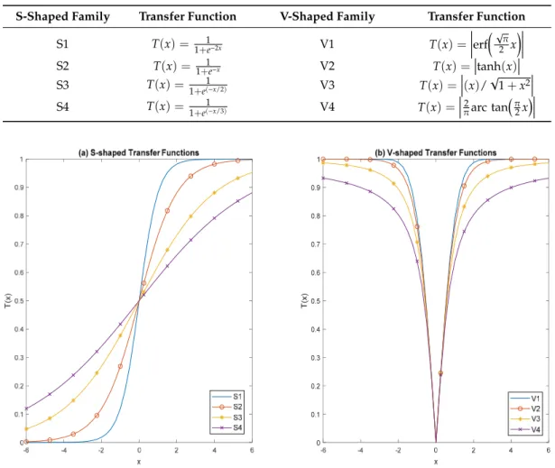
According to literature, the utilization of transfer function is one of the effective ways to convert continuous optimizer into a binary one. In comparison with other operators, the transfer function is cheaper, simple, and faster, which leads to the ease of implementation [18,19]. In most of the previous studies, researchers employed either S-shaped or V-shaped transfer function to convert the continuous optimizer to binary. Therefore, in this study, we use four S-shaped (S1–S4) and V-shaped (V1–V4) transfer functions to change the continuous HHO into the binary version. Table1shows the S-shaped and V-shaped transfer functions with mathematical definitions. The illustrations of S-shaped and V-shaped transfer functions are demonstrated in Figure2.

(6)

Electronics2019,8, 1130 6 of 27

Table 1.The utilized S-shaped and V-shaped transfer functions.

S-Shaped Family Transfer Function V-Shaped Family Transfer Function

S1 T(x) = ₁₊1_e−2x V1 T(x) = erf √ π 2 x S2 T(x) = ₁₊1_e−x V2 T(x) = tanh(x) S3 T(x) = 1 1+e(−x/2) V3 T(x) = (x)/ √ 1+x2 S4 T(x) = 1 1+e(−x/3) V4 T(x) = 2 πarc tan _π 2x

shaped and V-shaped transfer functions with mathematical definitions. The illustrations of S-shaped and V-S-shaped transfer functions are demonstrated in Figure 2.

Table 1. The utilized S-shaped and V-shaped transfer functions.

S-Shaped Family Transfer Function V-Shaped Family Transfer Function

S1

( )

2 1 1 x T x e− = + V1 T x

( )

erf 2 x π   = _ _   S2

( )

1 1 x T x e− = + V2 T x

( )

= tanh

( )

x S3

( )

₍ / 2₎ 1 1 x T x e− = + V3

( ) ( )

2 1 T x = x +x S4

( )

₍ /3₎ 1 1 x T x e− = + V4

( )

2 arc tan 2 T x π x π   = _ _

Figure 2. Sample S-shaped and V-shaped transfer functions. (a) S-shaped transfer fFunctions and (b) V-shaped transfer functions.

By integrating the transfer function into binary HHO (BHHO), the algorithm is able to perform the search on the binary search space. In BHHO, the position of the hawk is updated in two stages. In the first stage, BHHO updates the position of the hawk (Xid(t)) into a new position (∆Xid(t + 1)) similar to HHO. Note that the new position (∆Xid(t + 1)) is presenting in continuous form. In the second stage, the S-shaped or V-shaped transfer function is used to transform the new position into probability value. The new position of the hawk is then updated using Equation (17) or Equation (18). In this way, the position of the hawk can be expressed in binary form.

In S-shaped family, BHHO updates the new position of the hawk as follow [20]:

( )

1 1 if

( )

0,1

(

( )

1

)

0 otherwise d i d i rand T X t X t+ = < Δ +  (17)

Figure 2.Sample S-shaped and V-shaped transfer functions. (a) S-shaped transfer fFunctions and (b) V-shaped transfer functions.

By integrating the transfer function into binary HHO (BHHO), the algorithm is able to perform the search on the binary search space. In BHHO, the position of the hawk is updated in two stages. In the first stage, BHHO updates the position of the hawk (Xid(t)) into a new position (∆Xid(t+1)) similar to HHO. Note that the new position (∆Xid(t+1)) is presenting in continuous form. In the second stage, the S-shaped or V-shaped transfer function is used to transform the new position into probability value. The new position of the hawk is then updated using Equation (17) or Equation (18). In this way, the position of the hawk can be expressed in binary form.

In S-shaped family, BHHO updates the new position of the hawk as follow [20]:

Xd_i(t+1) =        1 ifrand(0, 1)<T∆Xd_i(t+1) 0 otherwise (17)

whereT(x) is the S-shaped transfer function,rand(0,1) is a random number in [0,1],Xis the position of the hawk,iis the order of hawk in the population,dis the dimension, andtis the current iteration.

Unlike the S-shaped transfer function, V-shaped transfer function does not force the search agent into 0 or 1. In V-shaped family, the new position of the hawk is updated as [21]:

Xd_i(t+1) =        ¬_Xd i(t) ifrand(0, 1)<T ∆Xd_i(t+1) X_id(t) otherwise (18)

(7)

whereT(x) is the V-shaped transfer function,rand(0,1) is a random number in [0,1],Xis the position of the hawk,iis the order of hawk in the population,dis the dimension,tis the current iteration, and¬_X is the complement ofX.

3.3. Binary Harris Hawk Optimization Algorithm

The pseudocode of BHHO is demonstrated in Algorithm 1. Algorithm 1.Binary Harris hawk optimization.

Inputs:NandT

1: Initialize theXiforNhawks

2: for(t=1 toT)

3: Evaluate the fitness value of the hawks,F(X) 4: Define the best solution asXr

5: for(i=1 toN)

6: Compute theE0andJas shown in (2) and (7), respectively

7: Update theEusing (1) //Exploration phase// 8: if(|E|≥₁₎

9: Update the position of the hawk using (3)

10: Calculate the probability using S-shaped or V-shaped transfer function 11: Update new position of the hawk using (17) or (18)

//Exploitation phase// 12: elseif(|E| <1)

//Soft besiege//

13: if(r≥_{0.5) and (}|_E|≥_0.5)

14: Update the position of the hawk as shown in (5)

//Hard besiege//

17: elseif(r≥_{0.5) and (}|_E| <_0.5)

//Soft besiege with progressive rapid dives// 21: elseif(r<0.5) and (|E|≥_0.5)

//Hard besiege with progressive rapid dives// 25: elseif(r<0.5) and (|E| <0.5)

29: end if 30: end if 31: nexti

32: UpdateXrif there is a better solution 33: nextt

Output: Global best solution

4. The Proposed Quadratic Binary Harris Hawk Optimization

In the previous section, the BHHO algorithms have discussed. However, in the experiment, we found that the performance of BHHO was still far from perfect. It shows that BHHO cannot efficiently

(8)

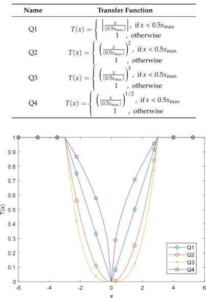
solve the feature selection problems. From the aforementioned, transfer function is one of the simplest and effective ways to convert the HHO into a binary one. However, the BHHO with S-shaped or V-shaped transfer function might not work effectively in feature selection tasks. In this regard, we propose the new quadratic binary Harris hawk optimization (QBHHO) to enhance the performance of BHHO in current work. Unlike BHHO, QBHHO utilizes the quadratic transfer function to convert the HHO into a binary one. In this work, we propose four quadratic transfer functions (Q1–Q4), as shown in Table2. Figure3presents the illustrations of quadratic transfer functions.

Table 2.The utilized quadratic transfer functions.

Name Transfer Function

Q1 T(x) =        x (0.5xmax) , ifx<0.5xmax 1 , otherwise Q2 T(x) =          x (0.5xmax) 2 , ifx<0.5xmax 1 , otherwise Q3 T(x) =          x (0.5xmax) 3 , ifx<0.5xmax 1 , otherwise Q4 T(x) =          x (0.5xmax) 1/2 , ifx<0.5xmax 1 , otherwise

4. The Proposed Quadratic Binary Harris Hawk Optimization

In the previous section, the BHHO algorithms have discussed. However, in the experiment, we found that the performance of BHHO was still far from perfect. It shows that BHHO cannot efficiently solve the feature selection problems. From the aforementioned, transfer function is one of the simplest and effective ways to convert the HHO into a binary one. However, the BHHO with S-shaped or V-shaped transfer function might not work effectively in feature selection tasks. In this regard, we propose the new quadratic binary Harris hawk optimization (QBHHO) to enhance the performance of BHHO in current work. Unlike BHHO, QBHHO utilizes the quadratic transfer function to convert the HHO into a binary one. In this work, we propose four quadratic transfer functions (Q1–Q4), as shown in Table 2. Figure 3 presents the illustrations of quadratic transfer functions.

Table 2. The utilized quadratic transfer functions.

Name Transfer function

Q1

( )

(

max

)

max , if 0.5 0.5 1 , otherwise x x x T x x  <  =   Q2

( )

(

)

2 max max , if 0.5 0.5 1 , otherwise x _x _x T x x   __ __ _< =_ _   Q3

( )

(

)

3 max max , if 0.5 0.5 1 , otherwise x _x _x T x x   __ __ _< =_ _   Q4

( )

(

)

1 2 max max , if 0.5 0.5 1 , otherwise x x x T x x   _ _ _<   =_ _  

Figure 3. Sample quadratic transfer functions with xmax = 6.

Figure 3.Sample quadratic transfer functions withxmax=6.

The QBHHO first updates the position of the hawk and then converts the new position into probability value using the quadratic transfer function. Afterward, the following rule is used for updating the hawk’s position [22]:

Xd_i(t+1) =        ¬_Xd i(t) ifrand(0, 1)<T ∆X_id(t+1) Xd_i(t) otherwise (19)

whereT(x) is the quadratic transfer function,rand(0,1) is a random number in [0,1],Xis the position of the hawk,iis the order of hawk in the population,dis the dimension,tis the current iteration, and¬_X is the complement ofX. The pseudocode of QBHHO is demonstrated in Algorithm 2.

(9)

Algorithm 2.Quadratic binary Harris hawk optimization. Inputs:NandT

1: Initialize theXiforNhawks

2: for(t=1 toT)

3: Evaluate the fitness value of the hawks,F(X) 4: Define the best solution asXr

5: for(i=1 toN)

6: Compute theE0andJas shown in (2) and (7), respectively

7: Update theEusing (1) //Exploration phase// 8: if(|E|≥₁₎

10: Calculate the probability using quadratic transfer function 11: Update new position of the hawk using (19)

//Exploitation phase// 12: elseif(|E| <1)

//Soft besiege//

13: if(r≥_{0.5) and (}|_E|≥_0.5)

//Hard besiege//

17: elseif(r≥_{0.5) and (}|_E| <_0.5)

//Soft besiege with progressive rapid dives// 21: elseif(r<0.5) and (|E|≥_0.5)

//Hard besiege with progressive rapid dives// 25: elseif(r<0.5) and (|E| <0.5)

29: end if 30: end if 31: nexti

32: UpdateXrif there is a better solution 33: nextt

Output: Global best solution

5. Application of Proposed BHHO and QBHHO for Feature Selection

In this section, the application of the proposed BHHO and QBHHO algorithms for the feature selection problems are presented. Generally, the feature selection problem is anNP-hard combinatorial binary optimization problem, in which the possible solutions increase exponentially with the number of features. LetDbe the total number of features. The number of possible solutions is 2D-1, which is impractical to perform the search exhaustively. Therefore, we propose the BHHO and QBHHO to automatically find the promising solution (feature subset) that can significantly improve the performance of the classification model.

(10)

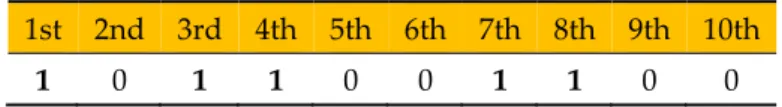
In feature selection, the solutions are representing in binary form, and they can be either bit ‘0’ or bit ‘1’. Bit ‘1’ indicates that the feature is selected, whereas bit ‘0’ represents the unselected feature [23]. Taking the sample solution (solution consists of 10 features) in Figure4as an example, it shows that a total of five features (1st, 3rd, 4th, 7th, and 8th) have been selected.

with the number of features. Let D be the total number of features. The number of possible solutions is 2D_{-1, which is impractical to perform the search exhaustively. Therefore, we propose the BHHO} and QBHHO to automatically find the promising solution (feature subset) that can significantly improve the performance of the classification model.

In feature selection, the solutions are representing in binary form, and they can be either bit ‘0’ or bit ‘1’. Bit ‘1’ indicates that the feature is selected, whereas bit ‘0’ represents the unselected feature [23]. Taking the sample solution (solution consists of 10 features) in Figure 4 as an example, it shows that a total of five features (1st, 3rd, 4th, 7th, and 8th) have been selected.

1st 2nd 3rd 4th 5th 6th 7th 8th 9th 10th

1 0 1 1 0 0 1 1 0 0

Figure 4. Sample solution with 10 dimensions.

In wrapper feature selection, a fitness function (objective function) is required to evaluate the individual solution. The primary goal of feature selection is to enhance prediction accuracy and to reduce the number of features. In this work, the fitness function that considers both criteria is utilized, and it is defined as [9]:

(

)

Fitness Function Error 1 S

F α α ↓ = + − (20) . No of wrongly predicted Error

Total number of instances

= (21)

where Error is the error rate computed by a learning algorithm, |S| is the length of feature subset, |F| is the total number of features, and α is a parameter used to control the influence of classification performance and feature size. In Equation (20), the first term is the classification performance, while the second term is the feature reduction.

6. Experiment and Results

6.1. Dataset

In this study, twenty-two benchmark datasets collected from the UCI machine learning repository are used to validate the performances of proposed approaches [24]. Table 3 outlines the datasets used in this work. For each individual dataset, the features are normalized between 0 and 1 to prevent the numerical problem.

6.2. Parameter Settings

In the present study, the k-nearest neighbor (KNN) algorithm with Euclidean distance and k = 5 is used to compute the error rate (first term of the fitness function). Different BHHO and QBHHO algorithms are employed to find the most informative feature subset. The algorithms are repeated 30 times with different random seeds. Besides, the K-fold cross-validation manner is applied to compute the error rate in the fitness function for preventing the overfitting [15]. In each of the 30 runs, the dataset is partitioned into K equal parts. One part is used for the testing set, while the remaining K – 1 parts are used for the training set. The procedure is repeated with K times using different parts for the testing and training sets, and the average results are recorded. Finally, the average statistical measurements are collected throughout 30 independent runs and displayed as the final results. In the previous works, KNN was shown to be faster, simpler, and ease of implement [13,25,26]. Thus, the KNN is chosen as the learning algorithm in this work.

All the experiments are executed on MATLAB 9.3 using a PC with an Intel Core i5-9400F CPU 2.90 GHz and 16.0 GB RAM. In this study, we set K = 10.The number of hawks (population size) is set to 10, and the maximum number of iterations is 100. This hyper-parameter setting was utilized in various previous works [27,28]. The dimension of search space is equal to the total number of features

Figure 4.Sample solution with 10 dimensions.

In wrapper feature selection, a fitness function (objective function) is required to evaluate the individual solution. The primary goal of feature selection is to enhance prediction accuracy and to reduce the number of features. In this work, the fitness function that considers both criteria is utilized, and it is defined as [9]:

↓_{Fitness Function}₌α_Error_{+ (}₁−α)|S|

|_F| (20)

Error= No.o f wrongly predicted

Total number o f instances (21)

whereErroris the error rate computed by a learning algorithm,|S|is the length of feature subset,|F| is the total number of features, andαis a parameter used to control the influence of classification performance and feature size. In Equation (20), the first term is the classification performance, while the second term is the feature reduction.

6. Experiment and Results 6.1. Dataset

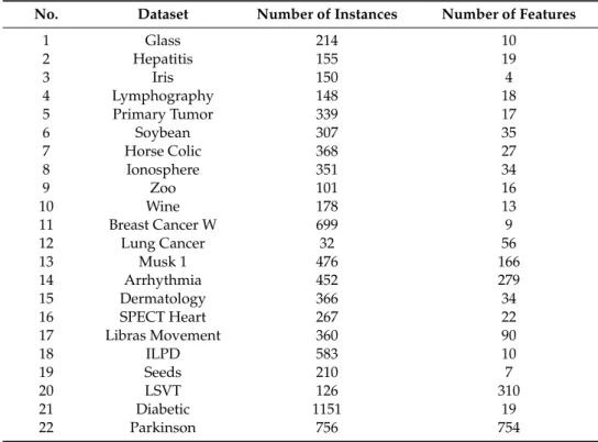
In this study, twenty-two benchmark datasets collected from the UCI machine learning repository are used to validate the performances of proposed approaches [24]. Table3outlines the datasets used in this work. For each individual dataset, the features are normalized between 0 and 1 to prevent the numerical problem.

6.2. Parameter Settings

In the present study, thek-nearest neighbor (KNN) algorithm with Euclidean distance andk=5 is used to compute the error rate (first term of the fitness function). Different BHHO and QBHHO algorithms are employed to find the most informative feature subset. The algorithms are repeated 30 times with different random seeds. Besides, theK-fold cross-validation manner is applied to compute the error rate in the fitness function for preventing the overfitting [15]. In each of the 30 runs, the dataset is partitioned intoKequal parts. One part is used for the testing set, while the remainingK– 1 parts are used for the training set. The procedure is repeated withKtimes using different parts for the testing and training sets, and the average results are recorded. Finally, the average statistical measurements are collected throughout 30 independent runs and displayed as the final results. In the previous works, KNN was shown to be faster, simpler, and ease of implement [13,25,26]. Thus, the KNN is chosen as the learning algorithm in this work.

All the experiments are executed on MATLAB 9.3 using a PC with an Intel Core i5-9400F CPU 2.90 GHz and 16.0 GB RAM. In this study, we setK=10. The number of hawks (population size) is set to 10, and the maximum number of iterations is 100. This hyper-parameter setting was utilized in various previous works [27,28]. The dimension of search space is equal to the total number of features of each dataset. According to [9,28,29], we choose theα=0.99 since the classification performance is the most important in the current work.

(11)

Table 3.The list of used datasets.

No. Dataset Number of Instances Number of Features

1 Glass 214 10 2 Hepatitis 155 19 3 Iris 150 4 4 Lymphography 148 18 5 Primary Tumor 339 17 6 Soybean 307 35 7 Horse Colic 368 27 8 Ionosphere 351 34 9 Zoo 101 16 10 Wine 178 13 11 Breast Cancer W 699 9 12 Lung Cancer 32 56 13 Musk 1 476 166 14 Arrhythmia 452 279 15 Dermatology 366 34 16 SPECT Heart 267 22 17 Libras Movement 360 90 18 ILPD 583 10 19 Seeds 210 7 20 LSVT 126 310 21 Diabetic 1151 19 22 Parkinson 756 754

6.3. Evaluation of Proposed BHHO and QBHHO Algorithms

In the first part of the experiment, the performances of the BHHO and QBHHO algorithms are validated on 22 datasets. The commonly used evaluation metrics include the best fitness value, mean fitness value, standard deviation of fitness value (STD), classification accuracy, and the number of selected features (feature size) are measured, and they can be defined as follows [9,30,31]:

Best Fitness=minR_m=₁Gbm (22)

Mean Fitness= 1 R R X m=1 Gbm (23) STD= s PR m=1(Gbm−µ) 2 R−₁ (24) Average accuracy= 1 R R X m=1

No.o f correctly predictedm

Total number o f instances (25)

Average feature size =1 R

R X

m=1

|_S|_m ₍₂₆₎

whereGbis the global best solution obtained from runm,µis the mean fitness,|S|is the number of selected features,mis the order of run, andRis the maximum number of runs.

(12)

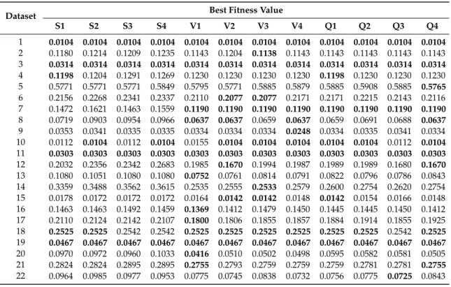
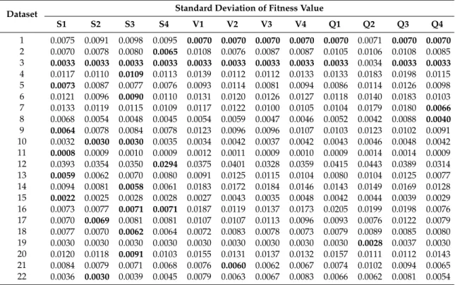
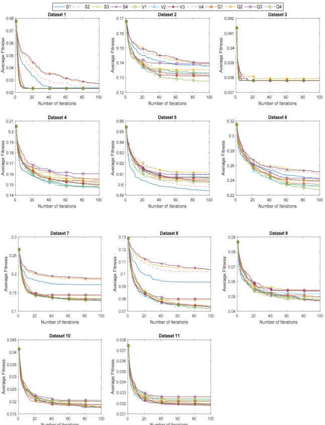
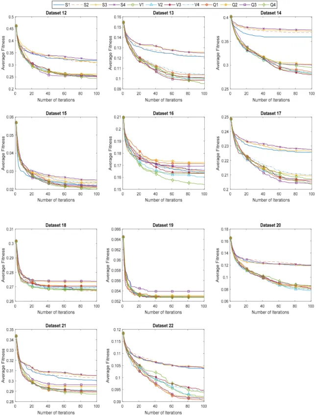
The twelve proposed approaches, BHHO (S1–S4 and V1–V4) and QBHHO (Q1–Q4) are compared to investigate the best binary version of HHO in feature selection. Tables4–6present the experimental results of the best, mean, and STD fitness values of proposed algorithms. In these tables, the best result is highlighted with bold text. In Table4, the BHHO-V1 scored the optimal best fitness value on most of the datasets (twelve datasets), followed by QBHHO-Q4 (11 datasets). From Table5, the best algorithm that contributed to the lowest mean fitness value was found to be QBHHO-Q4 (12 datasets), followed by BHHO-S1 and BHHO-S2 (five datasets). This shows that QBHHO-Q4 provided the highest diversity. On the one hand, BHHO-S3 perceived the most consistent results due to the lowest STD values in eight datasets. Furthermore, the convergence curves of the proposed algorithms on 22 datasets were shown in Figures5and6.

Tables7and8outline the result of the average classification accuracy and average feature size of the proposed algorithms. As can be observed, QBHHO-Q4 outperformed other algorithms in finding promising solutions, thus, leading to optimal classification accuracy. Among rivals, QBHHO-Q4 has achieved the highest average classification accuracy in eleven datasets. It shows that the quadratic transfer function can usually overtake S-shaped and V-shaped transfer functions in feature selection. On the other hand, QBHHO-Q2 provided the smallest number of selected features on most of the datasets, followed by BHHO-V4. Even though V-shaped transfer function can significantly reduce the number of features, however, the relevant features are eliminated and thus resulting in unsatisfactory performance. On the whole, QBHHO with quadratic transfer function Q4 is the best binary version of HHO in current work. Therefore, only QBHHO with transfer function Q4 is used in the rest of this paper.

Table 4.Experimental result of the best fitness value of the proposed algorithms.

Dataset Best Fitness Value

S1 S2 S3 S4 V1 V2 V3 V4 Q1 Q2 Q3 Q4 1 0.0104 0.0104 0.0104 0.0104 0.0104 0.0104 0.0104 0.0104 0.0104 0.0104 0.0104 0.0104 2 0.1180 0.1214 0.1209 0.1235 0.1143 0.1204 0.1138 0.1143 0.1143 0.1143 0.1143 0.1143 3 0.0314 0.0314 0.0314 0.0314 0.0314 0.0314 0.0314 0.0314 0.0314 0.0314 0.0314 0.0314 4 0.1198 0.1204 0.1291 0.1269 0.1230 0.1230 0.1230 0.1230 0.1198 0.1230 0.1230 0.1230 5 0.5771 0.5771 0.5771 0.5849 0.5795 0.5771 0.5885 0.5879 0.5885 0.5908 0.5885 0.5765 6 0.2156 0.2268 0.2341 0.2337 0.2110 0.2077 0.2077 0.2171 0.2171 0.2215 0.2143 0.2116 7 0.1472 0.1621 0.1463 0.1559 0.1190 0.1190 0.1190 0.1190 0.1190 0.1190 0.1190 0.1190 8 0.0719 0.0903 0.0954 0.0966 0.0637 0.0637 0.0659 0.0637 0.0659 0.0691 0.0688 0.0637 9 0.0353 0.0341 0.0335 0.0335 0.0334 0.0334 0.0334 0.0248 0.0334 0.0335 0.0341 0.0334 10 0.0112 0.0104 0.0112 0.0104 0.0155 0.0104 0.0104 0.0104 0.0104 0.0104 0.0112 0.0104 11 0.0303 0.0303 0.0303 0.0303 0.0303 0.0303 0.0303 0.0303 0.0303 0.0303 0.0303 0.0303 12 0.2032 0.2356 0.2342 0.2683 0.1985 0.1670 0.1994 0.1987 0.1989 0.1989 0.1680 0.1670 13 0.1080 0.1051 0.1080 0.1080 0.0752 0.0761 0.0814 0.0791 0.0822 0.0796 0.0786 0.0843 14 0.3359 0.3488 0.3562 0.3615 0.2535 0.2555 0.2533 0.2579 0.2600 0.2754 0.2620 0.2754 15 0.0178 0.0172 0.0172 0.0172 0.0164 0.0142 0.0142 0.0148 0.0142 0.0154 0.0166 0.0148 16 0.1463 0.1463 0.1492 0.1459 0.1369 0.1412 0.1479 0.1450 0.1445 0.1445 0.1450 0.1412 17 0.2110 0.2124 0.2142 0.2107 0.1800 0.1806 0.1855 0.1857 0.1884 0.1914 0.1855 0.1925 18 0.2525 0.2525 0.2542 0.2542 0.2525 0.2525 0.2525 0.2525 0.2525 0.2525 0.2542 0.2525 19 0.0467 0.0467 0.0467 0.0467 0.0467 0.0467 0.0467 0.0467 0.0467 0.0467 0.0467 0.0467 20 0.0970 0.0972 0.0960 0.1033 0.0416 0.0510 0.0502 0.0498 0.0595 0.0582 0.0581 0.0505 21 0.2824 0.2824 0.2895 0.2895 0.2755 0.2793 0.2759 0.2759 0.2759 0.2781 0.2781 0.2755 22 0.0964 0.0985 0.0977 0.0953 0.0775 0.0745 0.0838 0.0732 0.0756 0.0775 0.0725 0.0843

(13)

Table 5.Experimental result of the mean fitness value of the proposed algorithms.

Dataset Mean Fitness Value

S1 S2 S3 S4 V1 V2 V3 V4 Q1 Q2 Q3 Q4 1 0.0237 0.0250 0.0273 0.0270 0.0232 0.0232 0.0232 0.0232 0.0232 0.0233 0.0232 0.0232 2 0.1378 0.1382 0.1394 0.1402 0.1332 0.1327 0.1311 0.1331 0.1317 0.1353 0.1394 0.1276 3 0.0378 0.0378 0.0378 0.0378 0.0378 0.0378 0.0378 0.0378 0.0378 0.0379 0.0378 0.0378 4 0.1464 0.1500 0.1519 0.1546 0.1502 0.1469 0.1496 0.1513 0.1533 0.1554 0.1602 0.1474 5 0.5938 0.5978 0.6023 0.6030 0.6067 0.6073 0.6064 0.6100 0.6049 0.6114 0.6095 0.6019 6 0.2416 0.2484 0.2515 0.2516 0.2320 0.2323 0.2387 0.2393 0.2347 0.2400 0.2426 0.2275 7 0.1709 0.1865 0.1858 0.1885 0.1323 0.1304 0.1286 0.1320 0.1332 0.1412 0.1438 0.1272 8 0.0935 0.1019 0.1038 0.1036 0.0739 0.0740 0.0728 0.0725 0.0739 0.0790 0.0799 0.0717 9 0.0474 0.0462 0.0473 0.0471 0.0497 0.0513 0.0535 0.0484 0.0496 0.0541 0.0541 0.0477 10 0.0175 0.0176 0.0178 0.0177 0.0200 0.0199 0.0188 0.0188 0.0187 0.0201 0.0205 0.0180 11 0.0319 0.0318 0.0318 0.0318 0.0323 0.0324 0.0319 0.0322 0.0322 0.0324 0.0326 0.0319 12 0.3180 0.3089 0.3109 0.3214 0.2561 0.2530 0.2517 0.2538 0.2551 0.2617 0.2532 0.2431 13 0.1214 0.1215 0.1256 0.1248 0.1005 0.0997 0.1011 0.1043 0.1037 0.0983 0.0986 0.0951 14 0.3590 0.3686 0.3714 0.3739 0.2814 0.2835 0.2798 0.2821 0.2853 0.3020 0.3007 0.2950 15 0.0216 0.0223 0.0242 0.0251 0.0206 0.0221 0.0215 0.0236 0.0211 0.0234 0.0221 0.0199 16 0.1643 0.1633 0.1651 0.1657 0.1632 0.1603 0.1635 0.1667 0.1712 0.1723 0.1692 0.1540 17 0.2256 0.2272 0.2263 0.2276 0.2036 0.2054 0.2065 0.2100 0.2054 0.2094 0.2043 0.2069 18 0.2677 0.2671 0.2675 0.2678 0.2679 0.2698 0.2705 0.2693 0.2706 0.2733 0.2739 0.2683 19 0.0527 0.0527 0.0527 0.0527 0.0530 0.0529 0.0527 0.0527 0.0529 0.0531 0.0539 0.0527 20 0.1193 0.1200 0.1190 0.1202 0.0806 0.0779 0.0811 0.0790 0.0830 0.0845 0.0860 0.0854 21 0.3007 0.3030 0.3051 0.3055 0.2908 0.2909 0.2901 0.2893 0.2892 0.2946 0.2964 0.2873 22 0.1037 0.1042 0.1044 0.1039 0.0921 0.0903 0.0943 0.0944 0.0907 0.0916 0.0915 0.0936

Table 6.Experimental result of the STD of the proposed algorithms.

Dataset Standard Deviation of Fitness Value

S1 S2 S3 S4 V1 V2 V3 V4 Q1 Q2 Q3 Q4 1 0.0075 0.0091 0.0098 0.0095 0.0070 0.0070 0.0070 0.0070 0.0070 0.0071 0.0070 0.0070 2 0.0070 0.0078 0.0080 0.0065 0.0108 0.0076 0.0087 0.0087 0.0105 0.0106 0.0108 0.0085 3 0.0033 0.0033 0.0033 0.0033 0.0033 0.0033 0.0033 0.0033 0.0033 0.0034 0.0033 0.0033 4 0.0117 0.0110 0.0109 0.0113 0.0139 0.0112 0.0112 0.0133 0.0133 0.0183 0.0198 0.0115 5 0.0073 0.0087 0.0077 0.0076 0.0093 0.0114 0.0081 0.0094 0.0086 0.0114 0.0126 0.0098 6 0.0121 0.0096 0.0090 0.0110 0.0131 0.0120 0.0126 0.0127 0.0118 0.0140 0.0183 0.0103 7 0.0133 0.0119 0.0115 0.0109 0.0117 0.0122 0.0100 0.0105 0.0104 0.0179 0.0180 0.0066 8 0.0068 0.0054 0.0048 0.0045 0.0054 0.0059 0.0047 0.0046 0.0052 0.0042 0.0088 0.0040 9 0.0064 0.0078 0.0084 0.0078 0.0123 0.0096 0.0096 0.0107 0.0103 0.0123 0.0102 0.0091 10 0.0032 0.0030 0.0030 0.0035 0.0034 0.0042 0.0037 0.0042 0.0043 0.0046 0.0048 0.0042 11 0.0008 0.0009 0.0010 0.0009 0.0012 0.0011 0.0009 0.0010 0.0009 0.0014 0.0014 0.0009 12 0.0393 0.0354 0.0350 0.0294 0.0375 0.0401 0.0328 0.0359 0.0415 0.0443 0.0389 0.0314 13 0.0059 0.0062 0.0070 0.0080 0.0091 0.0125 0.0115 0.0104 0.0080 0.0104 0.0125 0.0077 14 0.0094 0.0081 0.0058 0.0061 0.0183 0.0172 0.0184 0.0146 0.0143 0.0149 0.0169 0.0128 15 0.0022 0.0025 0.0028 0.0028 0.0027 0.0043 0.0035 0.0048 0.0042 0.0044 0.0039 0.0029 16 0.0073 0.0077 0.0071 0.0071 0.0187 0.0119 0.0137 0.0173 0.0205 0.0199 0.0198 0.0076 17 0.0070 0.0069 0.0081 0.0081 0.0107 0.0107 0.0113 0.0096 0.0093 0.0076 0.0122 0.0079 18 0.0077 0.0070 0.0062 0.0064 0.0072 0.0083 0.0078 0.0073 0.0079 0.0089 0.0085 0.0080 19 0.0030 0.0030 0.0030 0.0030 0.0030 0.0030 0.0030 0.0030 0.0030 0.0028 0.0037 0.0030 20 0.0120 0.0118 0.0091 0.0103 0.0155 0.0131 0.0137 0.0132 0.0157 0.0111 0.0112 0.0143 21 0.0084 0.0079 0.0071 0.0068 0.0076 0.0060 0.0062 0.0067 0.0074 0.0102 0.0094 0.0065 22 0.0036 0.0030 0.0039 0.0045 0.0079 0.0063 0.0067 0.0083 0.0066 0.0062 0.0081 0.0054

(14)

Electronics 2019, 8, x FOR PEER REVIEW 14 of 27

Figure 5. Convergence curves of proposed algorithms on datasets 1–11.

(15)

Figure 6. Convergence curves of proposed algorithms on datasets 12–22.

(16)

Table 7.Experimental result of the average classification accuracy of the proposed algorithms.

Dataset Average Classification Accuracy

S1 S2 S3 S4 V1 V2 V3 V4 Q1 Q2 Q3 Q4 1 0.9771 0.9759 0.9737 0.9740 0.9776 0.9776 0.9776 0.9776 0.9776 0.9775 0.9776 0.9776 2 0.8647 0.8642 0.8633 0.8622 0.8676 0.8680 0.8700 0.8676 0.8691 0.8653 0.8609 0.8736 3 0.9664 0.9664 0.9664 0.9664 0.9664 0.9664 0.9664 0.9664 0.9664 0.9662 0.9664 0.9664 4 0.8588 0.8550 0.8529 0.8500 0.8519 0.8548 0.8524 0.8505 0.8488 0.8467 0.8417 0.8545 5 0.4074 0.4032 0.3986 0.3975 0.3923 0.3918 0.3927 0.3888 0.3944 0.3878 0.3901 0.3978 6 0.7631 0.7556 0.7516 0.7513 0.7692 0.7687 0.7622 0.7613 0.7668 0.7616 0.7584 0.7742 7 0.8297 0.8146 0.8157 0.8132 0.8671 0.8691 0.8709 0.8675 0.8662 0.8581 0.8555 0.8723 8 0.9082 0.9004 0.8990 0.8992 0.9265 0.9263 0.9275 0.9279 0.9264 0.9213 0.9205 0.9289 9 0.9580 0.9590 0.9573 0.9577 0.9543 0.9527 0.9503 0.9557 0.9543 0.9497 0.9500 0.9563 10 0.9880 0.9878 0.9876 0.9873 0.9845 0.9843 0.9855 0.9855 0.9857 0.9841 0.9841 0.9867 11 0.9736 0.9735 0.9735 0.9736 0.9723 0.9726 0.9732 0.9729 0.9727 0.9723 0.9720 0.9732 12 0.6833 0.6933 0.6911 0.6800 0.7422 0.7456 0.7467 0.7444 0.7433 0.7367 0.7456 0.7556 13 0.8833 0.8830 0.8786 0.8791 0.9004 0.9014 0.8998 0.8962 0.8972 0.9030 0.9025 0.9065 14 0.6401 0.6317 0.6299 0.6274 0.7162 0.7141 0.7177 0.7155 0.7122 0.6953 0.6965 0.7027 15 0.9853 0.9841 0.9816 0.9807 0.9831 0.9818 0.9821 0.9801 0.9829 0.9806 0.9820 0.9842 16 0.8401 0.8408 0.8385 0.8379 0.8382 0.8415 0.8382 0.8347 0.8301 0.8288 0.8322 0.8481 17 0.7775 0.7756 0.7767 0.7754 0.7959 0.7944 0.7931 0.7896 0.7943 0.7902 0.7954 0.7931 18 0.7339 0.7347 0.7342 0.7339 0.7330 0.7307 0.7301 0.7316 0.7300 0.7270 0.7263 0.7327 19 0.9510 0.9510 0.9510 0.9510 0.9506 0.9508 0.9510 0.9510 0.9508 0.9505 0.9495 0.9510 20 0.8853 0.8844 0.8853 0.8839 0.9194 0.9222 0.9189 0.9208 0.9169 0.9158 0.9142 0.9153 21 0.6998 0.6977 0.6956 0.6952 0.7090 0.7087 0.7096 0.7100 0.7104 0.7046 0.7027 0.7126 22 0.9018 0.9008 0.9003 0.9004 0.9089 0.9103 0.9067 0.9066 0.9104 0.9098 0.9095 0.9083

Table 8.Experimental result of the average feature size of the proposed algorithms.

Dataset Average Number of Selected Features

S1 S2 S3 S4 V1 V2 V3 V4 Q1 Q2 Q3 Q4 1 1.03 1.13 1.23 1.23 1.07 1.07 1.07 1.07 1.07 1.03 1.07 1.07 2 7.17 7.17 7.83 7.20 4.03 3.83 4.53 3.83 4.00 3.73 3.17 4.63 3 1.83 1.83 1.83 1.83 1.83 1.83 1.83 1.83 1.83 1.80 1.83 1.83 4 12.00 11.53 11.23 10.90 6.50 5.57 6.23 5.87 6.47 6.43 6.20 6.17 5 12.07 11.97 11.77 11.13 8.70 8.80 8.77 8.27 9.13 9.00 9.63 9.67 6 24.90 22.37 19.43 18.97 12.43 11.63 11.70 10.43 13.20 13.77 12.27 14.07 7 6.37 8.13 9.27 9.63 2.07 2.03 2.10 2.10 2.07 1.93 2.00 2.07 8 8.80 11.10 12.77 12.93 3.63 3.47 3.73 3.87 3.60 3.93 3.93 4.43 9 9.37 8.97 8.17 8.27 7.23 7.07 6.87 7.20 7.00 6.83 7.33 7.20 10 7.37 7.20 7.27 6.57 6.03 5.70 5.77 5.73 5.90 5.67 6.17 6.23 11 5.17 4.97 5.07 5.07 4.37 4.67 4.90 4.80 4.60 4.53 4.43 4.87 12 25.43 29.40 28.83 25.90 5.03 6.13 4.77 4.53 5.50 5.67 7.07 6.27 13 96.40 94.70 89.87 85.63 30.93 34.30 30.73 25.97 32.23 38.37 34.60 40.60 14 73.23 110.50 137.83 139.57 13.23 11.93 10.47 11.20 9.97 8.67 8.10 18.60 15 24.03 22.33 20.37 20.53 13.47 13.77 12.87 13.07 13.93 14.43 14.60 14.27 16 13.30 12.50 11.47 11.70 6.67 7.53 7.27 6.80 6.73 6.33 6.73 7.93 17 47.93 45.23 47.03 46.83 13.77 16.23 15.00 15.57 15.63 14.90 15.53 19.40 18 4.30 4.50 4.37 4.37 3.53 3.27 3.23 3.50 3.30 3.00 2.90 3.70 19 2.93 2.93 2.93 2.93 2.87 2.90 2.93 2.93 2.90 2.87 2.77 2.93 20 176.60 174.67 167.60 162.13 27.10 28.87 25.27 20.17 25.37 35.47 30.50 46.67 21 6.77 7.03 7.13 7.03 5.03 4.80 4.80 4.30 4.70 4.20 3.93 5.30 22 487.00 454.47 425.70 404.87 144.53 115.10 144.20 141.67 145.67 172.83 144.47 210.00

6.4. Comparison with Other Metaheuristic Algorithms

In the second part of the experiment, five recent and popular metaheuristic algorithms, including binary differential evolution (BDE) [32], binary flower pollination algorithm (BFPA) [33], binary multi-verse optimizer (BMVO) [14], binary salp swarm algorithm (BSSA) [28], and genetic algorithm (GA) [34], are applied to examine the efficacy and efficiency of proposed QBHHO in feature selection

(17)

problem. BDE is a variant of differential evolution (DE) that composes of differentiation, mutation, crossover, and selection process. BFPA is a binary version of flower pollination algorithm (FPA) in which the S2 transfer function is implemented for conversion. BMVO integrates the V4 transfer function to convert the continuous variables into the binary one. BSSA is a binary variant of the salp swarm algorithm (SSA) that implements the V3 transfer function. GA comprises of parent selection, crossover, and mutation operators. We utilize a simple GA with roulette wheel selection and single crossover for comparison. Table9lists the parameter settings of the utilized algorithms.

Table 9.Parameter settings of the utilized algorithms.

Algorithm Parameter Value

BDE Number of vectors,N 10

Maximum number of generations,T 100

Crossover rate,CR 0.9

BFPA Number of flowers,N 10

Maximum number of iterations,T 100

Switch probability,P 0.8

BSSA Number of salps,N 10

BMVO Number of universes,N 10

Coefficient,WEP [0.02, 1]

GA Number of chromosomes,N 10

Maximum number of generations,T 100

Crossover rate,CR 0.8

Mutation rate,MR 0.01

Tables10–12display the experimental results of the best, mean, and STD fitness values of six different algorithms. In these tables, the best results are bolded. Based on the results obtained, QBHHO was showing competitive performance in feature selection. In comparison with BDE, BFPA, BMVO, BSSA, and GA, QBHHO was highly capable in finding the nearly optimal solution. From Table10, QBHHO yielded the optimal best fitness value in fourteen datasets, which overwhelmed other competitors in this work. This result proves that the QBHHO with quadratic transfer function is helpful for assisting the algorithm to find the optimal solution. Moreover, QBHHO offered the lowest mean fitness values on most of the datasets. This again validates the efficacy of QBHHO in exploring the untried areas when finding the global optimum. In Table12, the BFPA perceived the smallest STD value in most cases, which contributed to a high consistent result. However, BFPA cannot find the optimal solution very well and thus leading to an ineffective result.

Figures7and8demonstrate the convergence curves of six different algorithms on 22 datasets. As can be seen, QBHHO can usually offer a high diversity. Taking dataset 7 (horse colic) and 21 (diabetic) as the examples, QBHHO converged faster to find the promising solution, which overtook other algorithms in feature selection. That is, QBHHO keeps tracking the global optimum, thus leading to a high quality solution. This can be interpreted due to some strong properties of HHO algorithm, and the superior of quadratic transfer function we made in QBHHO algorithm.

(18)

Table 10.Experimental result of the best fitness value of six different algorithms.

Dataset Best Fitness Value

QBHHO BDE BFPA BMVO BSSA GA

1 0.0104 0.0397 0.0104 0.0104 0.0104 0.0104 2 0.1143 0.1367 0.1301 0.1220 0.1265 0.1220 3 0.0314 0.0314 0.0314 0.0314 0.0314 0.0314 4 0.1230 0.1274 0.1215 0.1371 0.1377 0.1258 5 0.5765 0.5921 0.5801 0.5963 0.6035 0.5795 6 0.2116 0.2252 0.2324 0.2455 0.2568 0.2037 7 0.1190 0.1804 0.1801 0.1538 0.1190 0.1217 8 0.0637 0.0946 0.0975 0.0722 0.0694 0.0643 9 0.0334 0.0459 0.0353 0.0341 0.0433 0.0341 10 0.0104 0.0170 0.0104 0.0163 0.0104 0.0112 11 0.0303 0.0311 0.0303 0.0306 0.0303 0.0314 12 0.1670 0.2356 0.2381 0.2679 0.2654 0.1354 13 0.0843 0.0968 0.1080 0.1080 0.1077 0.0504 14 0.2754 0.3644 0.3711 0.3447 0.3291 0.3038 15 0.0148 0.0221 0.0150 0.0237 0.0237 0.0121 16 0.1412 0.1506 0.1506 0.1506 0.1506 0.1374 17 0.1925 0.2116 0.2121 0.2137 0.2113 0.1832 18 0.2525 0.2542 0.2525 0.2525 0.2573 0.2542 19 0.0467 0.0467 0.0467 0.0467 0.0467 0.0467 20 0.0505 0.0985 0.0887 0.0946 0.0993 0.0528 21 0.2755 0.3080 0.2927 0.2852 0.2848 0.2778 22 0.0843 0.0906 0.0960 0.0913 0.1006 0.0629

Table 11.Experimental result of the mean fitness value of six different algorithms.

Dataset Mean Fitness Value

1 0.0232 0.0626 0.0444 0.0259 0.0232 0.0301 2 0.1276 0.1534 0.1418 0.1390 0.1422 0.1409 3 0.0378 0.0387 0.0378 0.0378 0.0378 0.0379 4 0.1474 0.1662 0.1495 0.1580 0.1732 0.1563 5 0.6019 0.6122 0.5974 0.6101 0.6325 0.6058 6 0.2275 0.2580 0.2485 0.2633 0.2813 0.2230 7 0.1272 0.2390 0.2036 0.1736 0.1468 0.1469 8 0.0717 0.1133 0.1100 0.0955 0.0857 0.0814 9 0.0477 0.0615 0.0494 0.0522 0.0663 0.0544 10 0.0180 0.0257 0.0190 0.0196 0.0249 0.0214 11 0.0319 0.0336 0.0319 0.0321 0.0335 0.0331 12 0.2431 0.3328 0.3236 0.3228 0.3245 0.2377 13 0.0951 0.1226 0.1261 0.1243 0.1326 0.0746 14 0.2950 0.3786 0.3788 0.3641 0.3483 0.3269 15 0.0199 0.0317 0.0228 0.0291 0.0387 0.0204 16 0.1540 0.1780 0.1662 0.1675 0.1854 0.1618 17 0.2069 0.2283 0.2278 0.2262 0.2285 0.2059 18 0.2683 0.2893 0.2671 0.2702 0.2743 0.2737 19 0.0527 0.0588 0.0527 0.0527 0.0539 0.0553 20 0.0854 0.1166 0.1236 0.1155 0.1236 0.0839 21 0.2873 0.3247 0.3088 0.3010 0.3025 0.3048 22 0.0936 0.1000 0.1051 0.1050 0.1091 0.0780

(19)

Table 12.Experimental result of the STD of six different algorithms. Dataset Standard Deviation of Fitness Value

1 0.0070 0.0133 0.0124 0.0093 0.0070 0.0142 2 0.0085 0.0089 0.0072 0.0074 0.0088 0.0108 3 0.0033 0.0042 0.0033 0.0033 0.0033 0.0034 4 0.0115 0.0140 0.0114 0.0099 0.0129 0.0134 5 0.0098 0.0149 0.0087 0.0089 0.0136 0.0121 6 0.0103 0.0173 0.0109 0.0105 0.0157 0.0121 7 0.0066 0.0251 0.0116 0.0141 0.0194 0.0143 8 0.0040 0.0077 0.0046 0.0079 0.0070 0.0087 9 0.0091 0.0084 0.0063 0.0089 0.0110 0.0119 10 0.0042 0.0059 0.0032 0.0030 0.0061 0.0045 11 0.0009 0.0016 0.0008 0.0010 0.0015 0.0014 12 0.0314 0.0510 0.0338 0.0315 0.0302 0.0445 13 0.0077 0.0100 0.0083 0.0070 0.0103 0.0138 14 0.0128 0.0080 0.0044 0.0086 0.0085 0.0147 15 0.0029 0.0081 0.0030 0.0032 0.0066 0.0041 16 0.0076 0.0099 0.0067 0.0091 0.0117 0.0165 17 0.0079 0.0103 0.0093 0.0074 0.0082 0.0114 18 0.0080 0.0159 0.0072 0.0067 0.0065 0.0104 19 0.0030 0.0076 0.0030 0.0030 0.0037 0.0052 20 0.0143 0.0102 0.0105 0.0110 0.0130 0.0148 21 0.0065 0.0097 0.0057 0.0079 0.0075 0.0124 22 0.0054 0.0043 0.0046 0.0047 0.0039 0.0074

Table13presents the experimental results of the average classification accuracy of six different algorithms. Note that the best results are highlighted with bold text. According to the result in Table13, the average classification accuracy obtained by QBHHO was far superior to other competitors in most cases. Out of 22 datasets, QBHHO contributed to the highest average classification accuracy on at least twelve datasets. Figures9and10exhibit the results of boxplot of six different algorithms on 22 datasets. In these figures, the red line in the box represents the median value, and the symbol ‘+’ denotes the outlier. As can be seen, QBHHO scored the highest median value in most cases, which provided better classification performance than BDE, BMVO, GA, BSSA, and BFPA algorithms.

Table14outlines the experimental results of the average feature size of six different algorithms. Inspecting the result in Table14, QBHHO can often choose fewer features in most cases (15 datasets). Additionally, BSSA selected fewer features on nine datasets. Based on the results obtained, QBHHO was good at finding a smaller subset of relevant features, which led to high classification performance.

(20)

Electronics 2019, 8, x FOR PEER REVIEW 20 of 27

Figure 7. Convergence curves of six different algorithms on datasets 1–11.

(21)

Figure 8. Convergence curves of six different algorithms on datasets 12–22.

(22)

Table 13.Experimental result of the average classification accuracy of six different algorithms. Dataset Average Classification Accuracy

1 0.9776 0.9414 0.9576 0.9751 0.9776 0.9714 2 0.8736 0.8502 0.8613 0.8631 0.8580 0.8611 3 0.9664 0.9658 0.9664 0.9664 0.9664 0.9664 4 0.8545 0.8393 0.8557 0.8455 0.8290 0.8469 5 0.3978 0.3891 0.4036 0.3902 0.3667 0.3939 6 0.7742 0.7473 0.7557 0.7389 0.7211 0.7799 7 0.8723 0.7636 0.7988 0.8274 0.8528 0.8529 8 0.9289 0.8909 0.8935 0.9063 0.9146 0.9207 9 0.9563 0.9457 0.9560 0.9523 0.9383 0.9500 10 0.9867 0.9806 0.9861 0.9855 0.9802 0.9835 11 0.9732 0.9732 0.9738 0.9729 0.9712 0.9726 12 0.7556 0.6700 0.6789 0.6778 0.6733 0.7633 13 0.9065 0.8835 0.8789 0.8787 0.8691 0.9291 14 0.7027 0.6244 0.6235 0.6355 0.6492 0.6741 15 0.9842 0.9756 0.9836 0.9757 0.9664 0.9840 16 0.8481 0.8272 0.8379 0.8358 0.8176 0.8409 17 0.7931 0.7762 0.7759 0.7757 0.7717 0.7965 18 0.7327 0.7124 0.7352 0.7305 0.7258 0.7275 19 0.9510 0.9459 0.9510 0.9510 0.9497 0.9484 20 0.9153 0.8892 0.8814 0.8875 0.8769 0.9189 21 0.7126 0.6776 0.6924 0.6992 0.6965 0.6961 22 0.9083 0.9066 0.9002 0.8984 0.8930 0.9261

Table 14.Experimental result of the average feature size of six different algorithms. Dataset Average Number of Selected Features

1 1.07 4.57 2.40 1.20 1.07 1.80 2 4.63 9.63 8.63 6.57 3.17 6.50 3 1.83 1.93 1.83 1.83 1.83 1.87 4 6.17 12.80 11.90 9.07 7.03 8.50 5 9.67 12.60 11.93 10.80 9.43 9.80 6 14.07 27.60 22.97 16.80 18.10 17.67 7 2.07 13.33 12.00 7.40 2.80 3.33 8 4.43 17.80 15.70 9.20 3.93 9.77 9 7.20 12.40 9.27 7.97 8.40 7.80 10 6.23 8.40 6.83 6.80 6.90 6.57 11 4.87 6.40 5.37 4.80 4.50 5.40 12 6.27 34.03 31.77 21.13 6.37 18.83 13 40.60 120.70 104.23 70.67 50.40 73.60 14 18.60 189.53 169.40 90.93 28.53 119.30 15 14.27 25.67 22.27 17.37 18.37 15.30 16 7.93 15.20 12.63 10.73 10.60 9.40 17 19.40 60.33 53.60 37.90 22.00 39.50 18 3.70 4.57 4.97 3.37 2.80 3.93 19 2.93 3.63 2.93 2.93 2.83 2.97 20 46.67 214.37 190.10 129.03 55.47 112.40 21 5.30 10.47 8.27 6.00 3.87 7.43 22 210.00 569.33 477.77 338.67 241.80 364.70

(23)

Figure 9. Boxplot of six different algorithms on datasets 1–11.

(24)

Figure 10. Boxplot of six different algorithms on datasets 12–22.

Furthermore, we apply the Wilcoxon signed-rank test to examine whether the performance of the proposed QBHHO is significantly better than other algorithms in this work. In the Wilcoxon signed-rank test, if the p-value achieved is less than 0.05, then the performances of the two algorithms are significantly difference; otherwise, the performances of the two algorithms are similar. Table 15 exhibits the result of Wilcoxon signed-rank test with p-values. In this Table, the symbols “w/t/l” indicates that the proposed QBHHO was significantly better to (win), equal to (tie), and significantly worse to (lose) other algorithms. Note that the results with the p-value greater than 0.05 are

Figure 10.Boxplot of six different algorithms on datasets 12–22.

Furthermore, we apply the Wilcoxon signed-rank test to examine whether the performance of the proposed QBHHO is significantly better than other algorithms in this work. In the Wilcoxon signed-rank test, if thep-value achieved is less than 0.05, then the performances of the two algorithms are significantly difference; otherwise, the performances of the two algorithms are similar. Table15 exhibits the result of Wilcoxon signed-rank test withp-values. In this Table, the symbols “w/t/l” indicates that the proposed QBHHO was significantly better to (win), equal to (tie), and significantly worse to (lose) other algorithms. Note that the results with thep-value greater than 0.05 are underlined. Inspecting the result in Table15, the performance of QBHHO was significantly better than other

(25)

algorithms in most datasets. The results again verify the superiority of QBHHO to solve the feature selection problem in classification tasks. To sum up, the experiments show the excellent properties of QBHHO in terms of classification accuracy and feature size. As an instant conclusion, QBHHO is a useful tool, and it is appropriate to apply in rehabilitation, clinical, and engineering applications.

Table 15.P-values of Wilcoxon signed-rank test.

Dataset P-Value

BDE BFPA BMVO BSSA GA

1 0.00000 1.00×₁₀−5 _0.06250 _1.00000 _0.01563 2 0.00000 1.00×₁₀−5 _1.00×₁₀−5 _0.00000 _5.00×₁₀−5 3 0.01563 1.00000 1.00000 1.00000 1.00000 4 1.00×₁₀−5 _0.13054 _2.00×₁₀−5 _0.00000 _0.00029 5 0.00411 0.06503 0.00047 0.00000 0.14430 6 0.00000 0.00000 0.00000 0.00000 0.05982 7 0.00000 0.00000 0.00000 9.00×₁₀−5 _2.00×₁₀−5 8 0.00000 0.00000 0.00000 0.00000 2.00×₁₀−5 9 1.00×₁₀−5 _0.01557 _0.00605 _0.00000 _0.00203 10 6.00×₁₀−5 _0.13839 _0.11775 _4.00×₁₀−5 _0.00772 11 6.00×₁₀−5 _1.00000 _0.12378 _4.00×₁₀−5 _0.00028 12 0.00000 0.00000 0.00000 0.00000 0.92625 13 0.00000 0.00000 0.00000 0.00000 1.00×₁₀−5 14 0.00000 0.00000 0.00000 0.00000 0.00000 15 0.00000 0.00071 0.00000 0.00000 0.52355 16 0.00000 1.00×₁₀−5 _0.00000 _0.00000 _0.04429 17 0.00000 0.00000 0.00000 0.00000 0.44051 18 3.00×₁₀−5 _0.66882 _0.07104 _0.00033 _0.01761 19 4.00×₁₀−5 _1.00000 _1.00000 _0.06250 _0.00098 20 0.00000 0.00000 0.00000 0.00000 0.46528 21 0.00000 0.00000 0.00000 0.00000 2.00×₁₀−5 22 0.00011 0.00000 0.00000 0.00000 0.00000 w/t/l 22/0/0 15/7/0 16/6/0 19/3/0 12/7/3 7. Conclusions

In this paper, the BHHO and QBHHO algorithms are proposed to tackle the feature selection problem in classification tasks. The BHHO integrated S-shaped or V-shaped transfer function to convert the continuous HHO into the binary version. On the one hand, the quadratic transfer function is introduced in QBHHO to enhance the performance of BHHO in feature selection. The proposed algorithms are validated on 22 benchmark datasets in the UCI machine learning repository. The performances of proposed algorithms are evaluated based on the best fitness value, mean fitness value, standard deviation of fitness value, classification accuracy, and feature size. Among the BHHO and QBHHO algorithms, the QBHHO with quadratic transfer function Q4 offered the optimal performance in current work. Furthermore, the performance of QBHHO is compared with other algorithms, include BDE, BFPA, BMVO, BSSA, and GA. The experimental results show that our proposed QBHHO can usually achieve the highest classification accuracy as well as the smallest feature size when dueling with feature selection tasks. All in all, QBHHO is a powerful tool to solve the feature selection problem in classification tasks.

In the future, QBHHO can be applied to other feature selection and real-world problems. In addition, the classifiers such as support vector machine (SVM) and neural network (NN) can be implemented to enhance the performance of the current algorithm. Moreover, QBHHO can be employed to solve the other binary optimization problems such as knapsack problem and optimized neural network. Lastly, the quadratic transfer function can be integrated into other metaheuristic algorithms to solve binary optimization problems.