University of California, Berkeley
U.C. Berkeley Division of Biostatistics Working Paper Series
Year Paper
Super Learner In Prediction
Eric C. Polley
∗Mark J. van der Laan
†∗Division of Biostatistics, University of California, Berkeley, [email protected] †University of California - Berkeley, [email protected]
This working paper is hosted by The Berkeley Electronic Press (bepress) and may not be commer-cially reproduced without the permission of the copyright holder.
http://biostats.bepress.com/ucbbiostat/paper266 Copyright c2010 by the authors.
Super Learner In Prediction
Eric C. Polley and Mark J. van der LaanAbstract
Super learning is a general loss based learning method that has been proposed and analyzed theoretically in van der Laan et al. (2007). In this article we con-sider super learning for prediction. The super learner is a prediction method de-signed to find the optimal combination of a collection of prediction algorithms. The super learner algorithm finds the combination of algorithms minimizing the validated risk. The super learner framework is built on the theory of cross-validation and allows for a general class of prediction algorithms to be considered for the ensemble. Due to the previously established oracle results for the cross-validation selector, the super learner has been proven to represent an asymptot-ically optimal system for learning. In this article we demonstrate the practical implementation and finite sample performance of super learning in prediction.
1
Introduction
A common task in statistical data analysis is estimator selection for prediction. An outcome Yi is measured along with a set of covariatesWiand interest is in the regression function E(Y|W). For a given regression problem, it is possible to create a set of algorithms all estimating the same function but with some variety. An algorithm is an estimator that maps a data set ofnobservations (Wi, Yi),
i= 1, . . . , n, into a prediction function that can be used to map an inputW into a predicted value forY. The algorithms may differ in the subset of the covariates used, the basis functions, the loss functions, the searching algorithm, and the range of tuning parameters, among others. We prefer the more general notion estimator selection instead of model selection, since the formal meaning of model in the field of statistics is the set of possible probability distributions, while most algorithms are not indexed by a model choice.
Estimator selection is not limited to selecting only a single estimator. Recent work has demon-strated that an ensemble of the algorithms in the collection can outperform a single algorithm.
van der Laan et al. [2007] introduced the super learner for estimator selection and proved the optimality of such an method. The super learner is related to the stacking algorithm introduced in neural networks context by Wolpert [1992] and adapted to the regression context by Breiman
[1996b]. The stacking algorithm is examined inLeBlanc and Tibshirani[1996] and the relationship to the model-mix algorithm of Stone [1974] and the predictive sample-reuse method of Geisser
[1975] is discussed.
In this article, we demonstrate how the super learner algorithm, as outlined by van der Laan et al. [2007] as a general minimum loss based learning method, in the context of prediction can be implemented, and empirically demonstrate the advantage of such an ensemble method. After a review of the super learner algorithm, a sequence of simulations is presented to highlight properties of the super learner, in accordance with the theoretical optimality results of the super learner. Following the simulations, the super learner is demonstrated on a series of real data sets.
2
Super Learner
In this section the general super learner algorithm for prediction is described along with some of the specific recommendations for implementation. The details follow van der Laan et al. [2007] closely, although some of the notation has changed to be consistent with the rest of the article.
Observe the learning data setXi= (Yi, Wi), i= 1, . . . , nwhereY is the outcome of interest and
W is a p-dimensional set of covariates. The objective is to estimate the functionψ0(W) = E(Y|W). The function can be expressed as the minimizer of the expected loss:
ψ0(W) = arg min
ψ E [L(X, ψ(W))] (1)
where the loss function is often the squared error loss, L2 : (Y −ψ(W))2. For a given problem, a library of prediction algorithms can be proposed. A library is simply a collection of algorithms. The algorithms in the library should come from contextual knowledge and a large set of default algorithms. We use algorithm in the general sense as any mapping from the data into a predictor. The algorithms may range from a simple linear regression model to a multi-step algorithm involving
a predicted value we consider it a prediction algorithm. For example, the library may include least squares regression estimators for a large class of regression working models indexed by subsets of the covariates, algorithms indexed by set values of the fine-tuning parameters for a collection of values, algorithms using internal cross-validation to set fine-tuning parameters, algorithms coupled with screening procedures to reduce the dimension of the covariate vector, and so on. Denote the libraryL and the cardinality of LasK(n).
1. Fit each algorithm inLon the entire data setX ={Xi :i= 1, . . . , n}to estimate ˆΨk(W), k= 1, . . . , K(n).
2. Split the data set X into a training and validation sample, according to a V-fold cross-validation scheme: splits the ordered n observations into V-equal size groups, let the ν-th group be the validation sample, and the remaining group the training sample, ν = 1, . . . , V. Define T(ν) to be the νth training data split and V(ν) to be the corresponding validation data split. T(ν) =X \V(ν), ν = 1, . . . , V.
3. For theνthfold, fit each algorithm inLonT(ν) and save the predictions on the corresponding validation data, ˆΨk,T(ν)(Wi),Xi ∈V(ν) forν= 1, . . . , V.
4. Stack the predictions from each algorithm together to create a nby K matrix,
Z =
ˆ
Ψk,T(ν)(WV(ν)), ν= 1, . . . , V &k= 1, . . . , K
, where we used the notation WV(ν) = (Wi:Xi ∈V(ν)) for the covariate-vectors of the V(ν)-validation sample.
5. Propose a family of weighted combinations of the candidate estimators indexed by weight-vectorα: m(z|α) = K k=1 αkΨˆk,T(ν)(WV(ν)), αk≥0 ∀k, K k=1 αk= 1.
6. Determine theαthat minimizes the cross-validated risk of the candidate estimatorKk=1αkΨˆk over all allowed α-combinations:
ˆ α= arg min α n i=1 (Yi−m(zi|α))2.
7. Combine ˆα with ˆΨk(W), k= 1, . . . , K according to the family m(z|α) of weighted combina-tions to create the final super learner fit:
ˆ ΨSL(W) = K k=1 ˆ αkΨˆk(W)
The super learner theory does not place any restrictions on the family of weighted combinations used for ensembling the algorithms in the library. The restriction of the parameter space forαto be the convex combination of the algorithms in the library provides greater stability of the final super learner prediction. The convex combination is not only empirically motivated, but also supported by the theory. The oracle results for the super learner require a bounded loss function. Restricting to the convex combination implies that if each algorithm in the library is bounded, the convex combination will also be bounded.
Also contained within the family of the convex combinations is the possibility of selecting only one algorithm. The nodes of the convex hull:
Anode ={(1,0, . . . ,0),(0,1, . . . ,0), . . . ,(0,0, . . . ,1)},
correspond with selecting the single algorithm from the library that minimizes the V-fold cross-validated risk. This is the usual cross-validation selector we refer to as the discrete super learner since it is searching over a finite set for the algorithm weights (α). Although possible for the super learner to select only a single algorithm from the library, it typically selects a weighted average of the algorithms together in an ensemble.
Super learner performs asymptotically as well as best possible weighted combination
For convenience, we provide here a short summary of the oracle results established in previous articles. For detail, we refer to these articles as referred to invan der Laan et al.[2007]. The oracle result for the cross-validation selector among a family of candidate estimators was established in van der Laan and Dudoit [2003] for general bounded loss functions: see also van der Vaart et al. [2006] for unbounded loss functions with tails that are controlled by exponential bounds and infinite families of candidate estimators, and van der Laan et al. [2007] for its application to the super learner. This result proves (see above references for the precise statement of these implications) that, if the number of candidate estimators,K(n), is polynomial in sample size, then the cross-validation selector is either asymptotically equivalent with the oracle selector (based on sample of size of training samples), or it achieves the parametric rate logn/nfor convergence w.r.t.
d(ψ, ψ0) ≡ E0{L(ψ) −L(ψ0)}. So in most realistic scenarios, in which none of the candidate estimators achieve the rate of convergence one would have with an a priori correctly specified parametric model, the cross-validated selected estimator selector performs asymptotically exactly as well (up till a constant) as the oracle selected estimator. As a consequence, the super learner will perform asymptotically exactly as well (w.r.t. the loss based dissimilarity) as the best possible choice for the given data set among the family of weighted combinations of the estimators. In particular, this proves that, by including all competitors in the library of candidate estimators, the super learner will asymptotically outperform any of its competitors, even if the set of competitors is allowed to grow polynomial in sample size. This motivated our naming “super learner” since it provides a system of combining many estimators into an improved estimator.
3
Examples
To examine the performance of the super learner we start with a series of simulations and then demonstrate a super learner on a collection of real data sets. The simulations are intended to illustrate the application of the super learner algorithm and highlight some of the properties.
3.1 Simulations
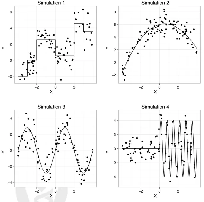
Four different simulations are presented in this section. All four simulations involve a univariateX drawn from a uniform distribution in [−4,+4]. The outcome follows the function described below:
Sim 1: Y =−2×I(X <−3) + 2.55×I(X >−2)−2×I(X >0) + 4×I(X >2)−1×I(X >3) +ε Sim 2: Y = 6 + 0.4X−0.36X2+ 0.005X3+ε Sim 3: Y = 2.83×sin π 2 ×X +ε Sim 4: Y = 4×sin (3π×X)×I(X >0) +ε
where I(·) is the usual indicator function andεis drawn from an independent standard normal dis-tribution in all simulations. A sample of size 100 will be drawn for each scenario. Figure 1 contains a scatterplot with a sample from each of the four simulations. The true curve for each simulation is represented by the solid line. These four simulations were chosen because they represent a diverse set of true models but all four have the same optimal R2 = 0.80. The R2 is computed as:
R2= 1− Yi− ˆ Yi 2 (Yi−ave(Yi))2 (2)
The optimalR2 is the value attained when the true regression function (i.e., true conditional mean) is used. Knowing the true regression function implies Yi−Yˆi2 = Var(ε)n= 1n. Hence the optimal R2 in all four simulations is R2opt = 1−1/Var(Y) and the variance of Y is set such that
Ropt2 = 0.80 in each simulation.
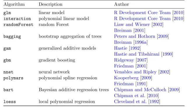
In all four simulations, we start with the same library of prediction algorithms. Table 1 contains a list of the algorithms in the library. The library of algorithms should ideally be a diverse set. One common aspect of many prediction algorithms is the need to specify values for tuning parameters. For example the generalized additive models requires a degree of freedom value for the spline functions or the neural network requires a size value. The tuning parameters could be selected using cross-validation or bootstrapping, but the different values of the tuning parameters could also be considered different prediction algorithms. A library could contain three generalized additive models with degrees of freedom equal to 2, 3, and 4. The selection of tuning parameters does not need to be done inside an algorithm, but each fixed value of a tuning parameter can be considered a different algorithm and the ensembling method can decide how to weight the different algorithms with unique values of the tuning parameters. When one considers different values of tuning parameters as unique prediction algorithms in the library it is easy to see how the number of algorithms in the library can become large. The library for the simulations contains 21 algorithms when considering different values of tuning parameters. A linear model and a linear model with a quadratic term are considered. The default random forest algorithm along with a collection of bagging regression trees with values of the complexity parameter equal to 0.10, 0.01, and 0.00 and a bagging algorithm adjusting the minimum split parameter to be 5 (with the default complexity parameter of 0.01). The generalized additive model with degrees of freedom equal to 2, 3, and 4 is added along with the default gradient boosting model. Neural networks with sizes 2 through 5, the polymars algorithm and the Bayesian additive regression trees is added. Finally, we consider the loess curve with spans equal to 0.75, 0.50, 0.25, and 0.10.
Simulation 1 X Y −2 0 2 4 6 ● ● ● ● ● ● ● ● ● ● ● ● ● ● ● ● ● ● ● ● ● ● ● ● ● ● ● ● ● ● ● ● ● ● ● ● ● ● ● ● ● ● ● ● ● ● ● ● ● ● ● ● ● ● ● ● ● ● ● ● ● ● ● ● ● ● ● ● ● ● ● ● ● ● ● ● ● ● ● ● ● ● ● ● ● ● ● ● ● ● ● ● ● ● ● ● ● ● ● ● −2 0 2 Simulation 2 X Y −2 0 2 4 6 8 ● ● ● ● ● ● ● ● ● ● ● ● ● ● ● ● ● ● ● ● ● ● ● ● ● ● ● ● ● ● ● ● ● ● ● ● ● ● ● ● ● ● ● ● ● ● ● ● ● ● ● ● ● ● ● ● ● ● ● ● ● ● ● ● ● ● ● ● ● ● ● ● ● ● ● ● ● ● ● ● ● ● ● ● ● ● ● ● ● ● ● ● ● ● ● ● ● ● ● ● −2 0 2 Simulation 3 X Y −4 −2 0 2 4 ● ● ● ● ● ● ● ● ● ● ● ● ● ● ● ● ● ● ● ● ● ● ● ● ● ● ● ● ● ● ● ● ● ● ● ● ● ● ● ● ● ● ● ● ● ● ● ● ● ● ● ● ● ● ● ● ● ● ● ● ● ● ● ● ● ● ● ● ● ● ● ● ● ● ● ● ● ● ● ● ● ● ● ● ● ● ● ● ● ● ● ● ● ● ● ● ● ● ● ● −2 0 2 Simulation 4 X Y −4 −2 0 2 4 ● ● ● ● ● ● ● ● ● ● ● ● ● ● ● ● ● ● ● ● ● ● ● ● ● ● ● ● ● ● ● ● ● ● ● ● ● ● ● ● ● ● ● ● ● ● ● ● ● ● ● ● ● ● ● ● ● ● ● ● ● ● ● ● ● ● ● ● ● ● ● ● ● ● ● ● ● ● ● ● ● ● ● ● ● ● ● ● ● ● ● ● ● ● ● ● ● −2 0 2
Figure 1: Scatterplots of the four simulations. The solid line is the true relationship. The points represent one of the simulation samples of size n= 100.
Table 1: Library of prediction algorithms for the simulations and citation for the correspondingR package.
Algorithm Description Author
glm linear model R Development Core Team[2010]
interaction polynomial linear model R Development Core Team[2010]
randomForest random Forest Liaw and Wiener[2002]
Breiman[2001]
bagging bootstrap aggregation of trees Peters and Hothorn [2009]
Breiman[1996a] gam generalized additive models Hastie[1992]
Hastie and Tibshirani [1990]
gbm gradient boosting Ridgeway[2007]
Friedman[2001]
nnet neural network Venables and Ripley [2002]
polymars polynomial spline regression Kooperberg [2009]
Friedman[1991]
bart Bayesian additive regression trees Chipman and McCulloch[2009]
Chipman et al. [2010]
loess local polynomial regression Cleveland et al.[1992]
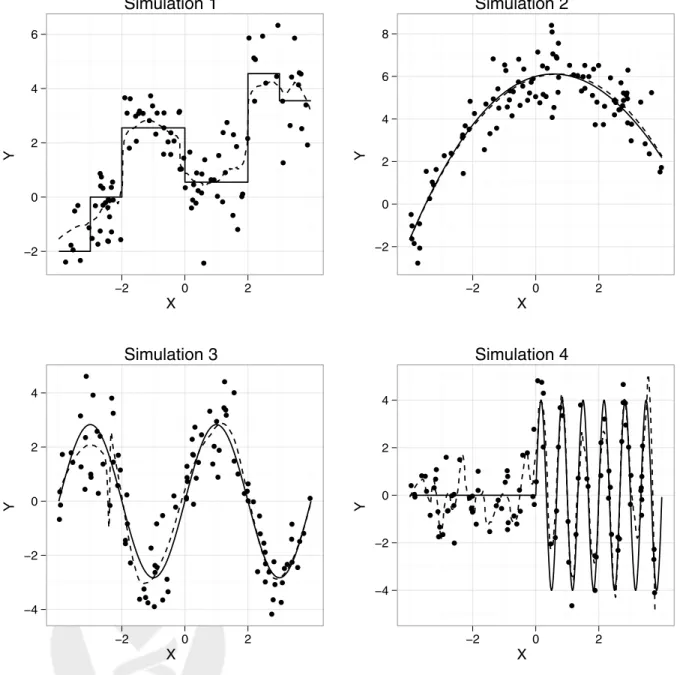
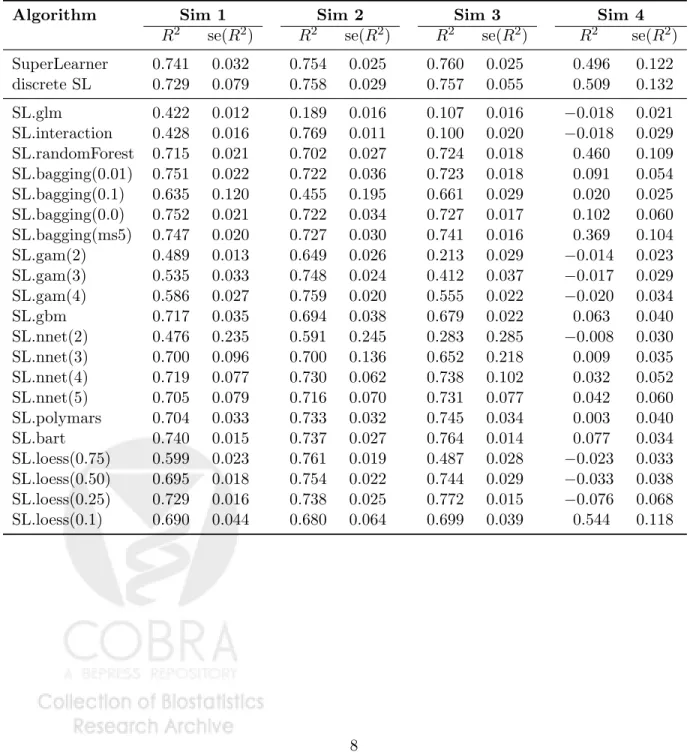
Figure 2 contains the super learner fit on a simulated data set for each scenario. With the given library the super learner is able to adapt to the underlying structure of the data generating function. For each algorithm we evaluated the R2 on a test set of size 10,000. To evaluate the performance of the super learner in comparison to each algorithm in the library, we simulated 100 samples of size 100 and computed the R2 for each fit of the true regression function. The results are presented in Table 2. In the first simulation, the regression tree based methods perform best. Bagging complete regression trees (cp = 0) has the largest R2. On the second simulation, the best algorithm is the quadratic linear regression model (SL.interaction). In both these cases the super learner is able to adapt to the underlying structure and is able to have an average R2 near the best. The same trend is exhibited in simulations 3 and 4, the super learner method of combining algorithms does nearly as well as the individual best algorithm. Since the individual best algorithm is not known, if a researcher was to select a single algorithm they might do well on some cases, but the overall performance will be worse than the super learner. For example, an individual who always uses bagging complete trees (SL.bagging(cp = 0.0)) will do well on the first 3 simulations, but will perform poorly on the 4th simulation compared to the average performance of the super learner.
The optimal R2 is the value attained by knowing the true regression function. The optimal value gives an upper bound on the possible R2 for each algorithm. In the first three simulations the super learner is able to come close to the optimal value because some of the algorithms in the library are able to well approximate the truth. But in the fourth simulation the library is not rich enough to contain a combination of algorithms able to approach the optimal value. The super learner is able to do as well as the best algorithms in the library but does not attain the optimal
Simulation 1 X Y −2 0 2 4 6 ● ● ● ● ● ● ● ● ● ● ● ● ● ● ● ● ● ● ● ● ● ● ● ● ● ● ● ● ● ● ● ● ● ● ● ● ● ● ● ● ● ● ● ● ● ● ● ● ● ● ● ● ● ● ● ● ● ● ● ● ● ● ● ● ● ● ● ● ● ● ● ● ● ● ● ● ● ● ● ● ● ● ● ● ● ● ● ● ● ● ● ● ● ● ● ● ● ● ● ● −2 0 2 Simulation 2 X Y −2 0 2 4 6 8 ● ● ● ● ● ● ● ● ● ● ● ● ● ● ● ● ● ● ● ● ● ● ● ● ● ● ● ● ● ● ● ● ● ● ● ● ● ● ● ● ● ● ● ● ● ● ● ● ● ● ● ● ● ● ● ● ● ● ● ● ● ● ● ● ● ● ● ● ● ● ● ● ● ● ● ● ● ● ● ● ● ● ● ● ● ● ● ● ● ● ● ● ● ● ● ● ● ● ● ● −2 0 2 Simulation 3 X Y −4 −2 0 2 4 ● ● ● ● ● ● ● ● ● ● ● ● ● ● ● ● ● ● ● ● ● ● ● ● ● ● ● ● ● ● ● ● ● ● ● ● ● ● ● ● ● ● ● ● ● ● ● ● ● ● ● ● ● ● ● ● ● ● ● ● ● ● ● ● ● ● ● ● ● ● ● ● ● ● ● ● ● ● ● ● ● ● ● ● ● ● ● ● ● ● ● ● ● ● ● ● ● ● ● ● −2 0 2 Simulation 4 X Y −4 −2 0 2 4 ● ● ● ● ● ● ● ● ● ● ● ● ● ● ● ● ● ● ● ● ● ● ● ● ● ● ● ● ● ● ● ● ● ● ● ● ● ● ● ● ● ● ● ● ● ● ● ● ● ● ● ● ● ● ● ● ● ● ● ● ● ● ● ● ● ● ● ● ● ● ● ● ● ● ● ● ● ● ● ● ● ● ● ● ● ● ● ● ● ● ● ● ● ● ● ● ● −2 0 2
Figure 2: Scatterplots of the four simulations. The solid line is the true relationship. The points represent one of the simulated datasets of sizen= 100. The dashed line is the super learner fit for the shown dataset.
Table 2: Results for all 4 simulations. Average R-squared based on 100 simulations and the corresponding standard errors.
Algorithm Sim 1 Sim 2 Sim 3 Sim 4
R2 se(R2) R2 se(R2) R2 se(R2) R2 se(R2) SuperLearner 0.741 0.032 0.754 0.025 0.760 0.025 0.496 0.122 discrete SL 0.729 0.079 0.758 0.029 0.757 0.055 0.509 0.132 SL.glm 0.422 0.012 0.189 0.016 0.107 0.016 −0.018 0.021 SL.interaction 0.428 0.016 0.769 0.011 0.100 0.020 −0.018 0.029 SL.randomForest 0.715 0.021 0.702 0.027 0.724 0.018 0.460 0.109 SL.bagging(0.01) 0.751 0.022 0.722 0.036 0.723 0.018 0.091 0.054 SL.bagging(0.1) 0.635 0.120 0.455 0.195 0.661 0.029 0.020 0.025 SL.bagging(0.0) 0.752 0.021 0.722 0.034 0.727 0.017 0.102 0.060 SL.bagging(ms5) 0.747 0.020 0.727 0.030 0.741 0.016 0.369 0.104 SL.gam(2) 0.489 0.013 0.649 0.026 0.213 0.029 −0.014 0.023 SL.gam(3) 0.535 0.033 0.748 0.024 0.412 0.037 −0.017 0.029 SL.gam(4) 0.586 0.027 0.759 0.020 0.555 0.022 −0.020 0.034 SL.gbm 0.717 0.035 0.694 0.038 0.679 0.022 0.063 0.040 SL.nnet(2) 0.476 0.235 0.591 0.245 0.283 0.285 −0.008 0.030 SL.nnet(3) 0.700 0.096 0.700 0.136 0.652 0.218 0.009 0.035 SL.nnet(4) 0.719 0.077 0.730 0.062 0.738 0.102 0.032 0.052 SL.nnet(5) 0.705 0.079 0.716 0.070 0.731 0.077 0.042 0.060 SL.polymars 0.704 0.033 0.733 0.032 0.745 0.034 0.003 0.040 SL.bart 0.740 0.015 0.737 0.027 0.764 0.014 0.077 0.034 SL.loess(0.75) 0.599 0.023 0.761 0.019 0.487 0.028 −0.023 0.033 SL.loess(0.50) 0.695 0.018 0.754 0.022 0.744 0.029 −0.033 0.038 SL.loess(0.25) 0.729 0.016 0.738 0.025 0.772 0.015 −0.076 0.068 SL.loess(0.1) 0.690 0.044 0.680 0.064 0.699 0.039 0.544 0.118
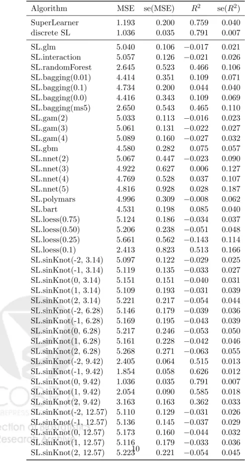
For the fourth simulation example, if the researcher thought that the relationship between X and Y followed a linear model up to a knot point, and then was a sine curve with an unknown frequency and amplitude, they could augment the library with proposed prediction algorithms:
sinKnot(X;k, ω) ={β1+β2X} ×I(X < k) (3) +{β3+β4sin(ωX)} ×I(X≥k)
for fixed values of the knot k and the frequency ω. For the fourth simulation, we augmented the library with the regression model above selecting values for the knots in {−2,−1,0,+1,+2} and values for the frequency in {π,2π,3π,4π} and all pairwise combinations of the two tuning parameters. This added 20 algorithms to the library (for a total of 41 algorithms). The results are presented in table 3. The 20 knot plus sine curve functions are labeled sinKnot(k, ω) in the table. The algorithm containing the true relationship between X and Y is sinKnot(0, 3π). The super learner now achieves a performance very close to the optimal R2.
3.2 Data Analysis
To study the super learner in real data examples, we collected a set of publicly available data sets. Table 4 contains a descriptions of the data sets used for the study. The sample sizes ranged from 200 to 654 observations and the number of covariates ranged from 3 to 18. All 13 data sets have a continuous outcome and no missing values. The data sets can be found either in public repositories like the UCI data repository or in textbooks, with the corresponding citation listed in the table.
For the library of prediction algorithms, the applicable algorithms from the univariate simula-tions along with the algorithms listed in table 5. These algorithms represent a diverse set of basis functions and should allow the super learner to work well in most real settings. For the comparison across all data sets, we kept the library of algorithms the same. The super learner may benefit from including algorithms based on contextual knowledge of the data problem as demonstrated in the augmented library in simulation 4.
Each data set has a different scale for the outcome. In order to compare the performance of the prediction algorithms across diverse data sets we used the relative mean squared error where the denominator is the mean squared error of a linear model:
relM SE(k) = M SE(k)
M SE(lm), k= 1, . . . , K (4)
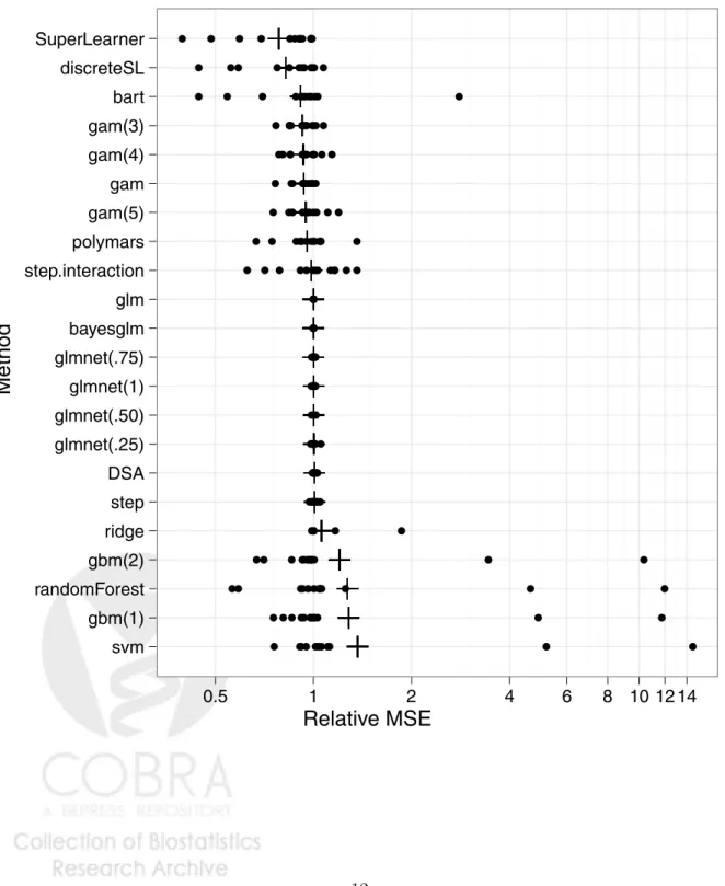
The results for the super learner, the discrete super learner, and each individual algorithm can be found in figure 3. Each point represents the 10-fold cross-validated relative mean squared error for a data set and the plus sign is the geometric mean of the algorithm across all 13 data sets. The super learner slightly outperforms the discrete super learner but both outperform any individual algorithm. With the real data it is unlikely that one single algorithm contains the true relationship and the benefit of the combination of the algorithms versus the selection of a single algorithm is demonstrated. The additional estimation of the combination parameters (α) does not appear to cause an over-fit in terms of the risk assessment. Among the individual library algorithms the
Table 3: Simulation results for example 2. Average mean squared error and R-squared based on 100 simulations and the corresponding standard errors.
Algorithm MSE se(MSE) R2 se(R2) SuperLearner 1.193 0.200 0.759 0.040 discrete SL 1.036 0.035 0.791 0.007 SL.glm 5.040 0.106 −0.017 0.021 SL.interaction 5.057 0.126 −0.021 0.026 SL.randomForest 2.645 0.523 0.466 0.106 SL.bagging(0.01) 4.414 0.351 0.109 0.071 SL.bagging(0.1) 4.734 0.200 0.044 0.040 SL.bagging(0.0) 4.416 0.343 0.109 0.069 SL.bagging(ms5) 2.650 0.543 0.465 0.110 SL.gam(2) 5.033 0.113 −0.016 0.023 SL.gam(3) 5.061 0.131 −0.022 0.027 SL.gam(4) 5.089 0.160 −0.027 0.032 SL.gbm 4.580 0.282 0.075 0.057 SL.nnet(2) 5.067 0.447 −0.023 0.090 SL.nnet(3) 4.922 0.627 0.006 0.127 SL.nnet(4) 4.769 0.528 0.037 0.107 SL.nnet(5) 4.816 0.928 0.028 0.187 SL.polymars 4.996 0.309 −0.008 0.062 SL.bart 4.531 0.198 0.085 0.040 SL.loess(0.75) 5.124 0.186 −0.034 0.037 SL.loess(0.50) 5.206 0.238 −0.051 0.048 SL.loess(0.25) 5.661 0.562 −0.143 0.114 SL.loess(0.1) 2.413 0.823 0.513 0.166 SL.sinKnot(-2, 3.14) 5.097 0.122 −0.029 0.025 SL.sinKnot(-1, 3.14) 5.119 0.135 −0.033 0.027 SL.sinKnot(0, 3.14) 5.151 0.151 −0.040 0.031 SL.sinKnot(1, 3.14) 5.109 0.193 −0.031 0.039 SL.sinKnot(2, 3.14) 5.221 0.217 −0.054 0.044 SL.sinKnot(-2, 6.28) 5.146 0.179 −0.039 0.036 SL.sinKnot(-1, 6.28) 5.169 0.195 −0.043 0.039 SL.sinKnot(0, 6.28) 5.217 0.246 −0.053 0.050 SL.sinKnot(1, 6.28) 5.161 0.228 −0.042 0.046 SL.sinKnot(2, 6.28) 5.268 0.271 −0.063 0.055 SL.sinKnot(-2, 9.42) 2.405 0.064 0.515 0.013 SL.sinKnot(-1, 9.42) 1.854 0.058 0.626 0.012 SL.sinKnot(0, 9.42) 1.036 0.035 0.791 0.007 SL.sinKnot(1, 9.42) 2.054 0.090 0.585 0.018 SL.sinKnot(2, 9.42) 3.163 0.163 0.362 0.033 SL.sinKnot(-2, 12.57) 5.110 0.129 −0.031 0.026 SL.sinKnot(-1, 12.57) 5.136 0.145 −0.037 0.029 SL.sinKnot(0, 12.57) 5.173 0.160 −0.044 0.032
Table 4: Description of data sets. n is the sample size and p is the number of covariates. All examples have a continuous outcome.
Name n p Source
ais 202 10 Cook and Weisberg[1994]
diamond 308 17 Chu[2001]
cps78 550 18 Berndt[1991] cps85 534 17 Berndt[1991] cpu 209 6 Kibler et al. [1989]
FEV 654 4 Rosner [1999]
Pima 392 7 Newman et al. [1998] laheart 200 10 Afifi and Azen[1979]
mussels 201 3 Cook [1998]
enroll 258 6 Liu and Stengos[1999] fat 252 14 Penrose et al. [1985] diabetes 366 15 Harrell[2001] house 506 13 Newman et al. [1998]
super learner which demonstrates the advantage of combining algorithms over selecting a single algorithm.
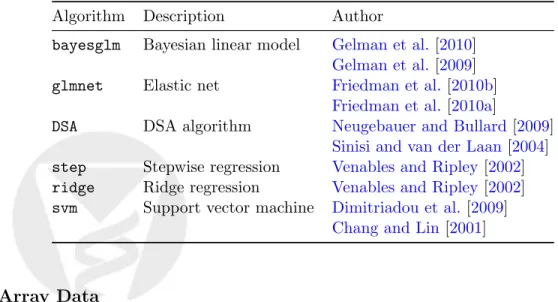
Table 5: Additional prediction algorithms in the library for the real data examples to be combined with the algorithms from Table 1.
Algorithm Description Author
bayesglm Bayesian linear model Gelman et al. [2010]
Gelman et al. [2009]
glmnet Elastic net Friedman et al. [2010b]
Friedman et al. [2010a]
DSA DSA algorithm Neugebauer and Bullard[2009]
Sinisi and van der Laan[2004] step Stepwise regression Venables and Ripley [2002]
ridge Ridge regression Venables and Ripley [2002]
svm Support vector machine Dimitriadou et al.[2009]
Chang and Lin [2001]
3.3 Array Data
Figure 3: 10-fold cross-validated relative mean squared error compared to glm across 13 real datasets. Sorted by the geometric mean, denoted with the plus (+) sign.
Relative MSE
Method
svm gbm(1) randomForest gbm(2) ridge step DSA glmnet(.25) glmnet(.50) glmnet(1) glmnet(.75) bayesglm glm step.interaction polymars gam(5) gam gam(4) gam(3) bart discreteSL SuperLearner ● ● ● ● ●●● ●● ● ●● ● ● ● ● ● ●●● ●●●● ●● ● ● ●● ● ●● ●● ●● ● ● ● ● ● ● ● ● ●●●●●● ● ● ● ● ● ● ● ● ●●● ● ●● ●● ●● ●●● ●●●●●● ●● ●●● ●● ● ●●●●● ●● ● ● ●● ●● ●●● ●● ●● ● ● ●● ●●●●● ●● ●● ● ● ●● ●●●●● ●● ●●●●●● ●●●●● ●● ● ● ● ● ● ● ● ● ● ● ● ● ● ● ● ● ● ● ● ● ● ● ● ● ● ● ● ● ● ●●● ●● ●●●● ● ● ● ● ●●● ●●●●●● ● ● ● ● ●●● ● ●●●●● ● ●●●● ● ●● ●●●● ●● ● ●● ●●●● ● ●●●● ● ● ● ●● ●●● ● ●●● ●● ● ● ● ● ●● ●● ●●●●● ● ● ●● ●●● ●●●●●● ● ● ● ● ● ●●●●● ●●● 0.5 1 2 4 6 8 10 12 14chosen the same.
The super learner in a microarray example is demonstrated using two publicly available data sets. The breast cancer data fromvan’t Veer et al. [2002] and the prostate cancer array data from
Singh et al. [2002]. The breast cancer study was conducted to develop a gene expression based predictor for 5 year distant metastases. The outcome in this case is a binary indicator that patient had a distant metastases within 5 years after initial therapy. In addition to the expression data, six clinical variables were attained. The clinical information is age, tumor grade, tumor size, estrogen receptor status, progesterone receptor status and angioinvasion. The array data contains 4348 genes after the unsupervised screening steps outlined in the original article. We used the entire sample of 97 individuals (combining the training and validation samples from the original article) to fit the super learner.
The prostate cancer study was conducted to develop a gene expression based predictor of a cancerous tumor. 102 tissue samples were collected with 52 from cancer tissue and 50 from non-cancer tissue. The data set contains 6033 genes after the pre-processing steps, but no clinical variables were available in the data set.
One aspect of high dimensional data analysis is that it is often beneficial to screen the variables before running the prediction algorithms. With the super learner framework, screening of variables can be either supervised or unsupervised since the screening step will be part of the cross-validation step. Screening algorithms can be coupled with prediction algorithms to create new algorithms in the library. For example, we may consider k-nearest neighbors using all features and on the subset of only clinical variables. These two algorithms can be considered unique algorithms in the super learner library. Another screening algorithm we consider is to test the pairwise correlations of each variable with the outcome and rank the variables by the corresponding p-value. With the ranked list of variables, we consider the screening cutoffs as: variables with a p-value less than 0.1, variables with a p-value less than 0.01, variables in the bottom 20, and variables in the bottom 50. An additional screening algorithm is to run the glmnet algorithm and select the variables with non-zero coefficients.
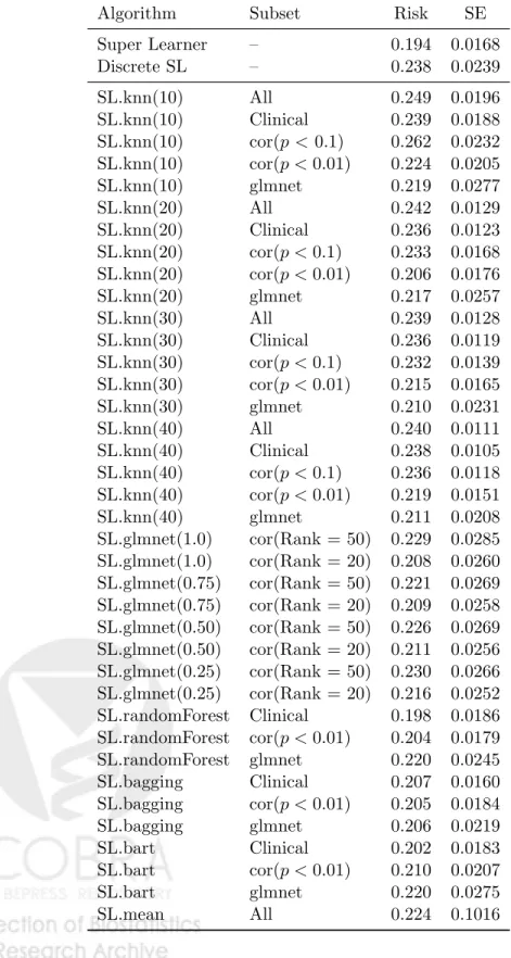
The results for the breast cancer data can be found in table 6. The algorithms in the library are k-nearest neighbors with k = {10, 20, 30, 40}, elastic net with α ={1.0,0.75,0.50,0.25}, random forests, bagging, bart, and an algorithm that uses the mean value of the outcome as the predicted probability. We coupled these algorithms with the screening algorithms to produce the full list of 38 algorithms. Within the library of algorithms, the best algorithm in terms of minimum risk estimate is the random forest algorithm using only the clinical variables (MSE = 0.198). As we observed in the previous examples, the super learner is able to attain a risk comparable to the best algorithm (MSE = 0.194).
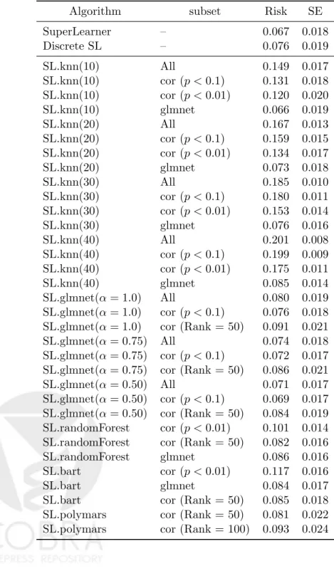
The results from the prostate cancer data can be found in table 7. The library of algorithms is similar to that used in the breast cancer example minus the clinical variable screening. In this example, the elastic net algorithm performs best among the library algorithms. The mean squared error for the elastic net fit with fine-tuning parameter alpha equal to 0.50, and fit on the entire data set, was 0.071. The super learner outperforms even the best algorithm in the library here with a mean squared error of 0.067.
Standard errors of the cross-validated risk are based on the results of Theorem 3 inDudoit and van der Laan [2005]. The equation for the estimator of the variance of the cross-validated risk of
Table 6: 20-fold cross-validated mean squared error for each algorithm and the standard error for the breast cancer study.
Algorithm Subset Risk SE
Super Learner – 0.194 0.0168 Discrete SL – 0.238 0.0239 SL.knn(10) All 0.249 0.0196 SL.knn(10) Clinical 0.239 0.0188 SL.knn(10) cor(p < 0.1) 0.262 0.0232 SL.knn(10) cor(p <0.01) 0.224 0.0205 SL.knn(10) glmnet 0.219 0.0277 SL.knn(20) All 0.242 0.0129 SL.knn(20) Clinical 0.236 0.0123 SL.knn(20) cor(p <0.1) 0.233 0.0168 SL.knn(20) cor(p <0.01) 0.206 0.0176 SL.knn(20) glmnet 0.217 0.0257 SL.knn(30) All 0.239 0.0128 SL.knn(30) Clinical 0.236 0.0119 SL.knn(30) cor(p <0.1) 0.232 0.0139 SL.knn(30) cor(p <0.01) 0.215 0.0165 SL.knn(30) glmnet 0.210 0.0231 SL.knn(40) All 0.240 0.0111 SL.knn(40) Clinical 0.238 0.0105 SL.knn(40) cor(p <0.1) 0.236 0.0118 SL.knn(40) cor(p <0.01) 0.219 0.0151 SL.knn(40) glmnet 0.211 0.0208 SL.glmnet(1.0) cor(Rank = 50) 0.229 0.0285 SL.glmnet(1.0) cor(Rank = 20) 0.208 0.0260 SL.glmnet(0.75) cor(Rank = 50) 0.221 0.0269 SL.glmnet(0.75) cor(Rank = 20) 0.209 0.0258 SL.glmnet(0.50) cor(Rank = 50) 0.226 0.0269 SL.glmnet(0.50) cor(Rank = 20) 0.211 0.0256 SL.glmnet(0.25) cor(Rank = 50) 0.230 0.0266 SL.glmnet(0.25) cor(Rank = 20) 0.216 0.0252 SL.randomForest Clinical 0.198 0.0186 SL.randomForest cor(p <0.01) 0.204 0.0179 SL.randomForest glmnet 0.220 0.0245 SL.bagging Clinical 0.207 0.0160 SL.bagging cor(p <0.01) 0.205 0.0184 SL.bagging glmnet 0.206 0.0219 SL.bart Clinical 0.202 0.0183 SL.bart cor(p <0.01) 0.210 0.0207 SL.bart glmnet 0.220 0.0275 SL.mean All 0.224 0.1016
Table 7: 20-fold cross-validated mean squared error for each algorithm and the standard error for the prostate cancer study.
Algorithm subset Risk SE
SuperLearner – 0.067 0.018 Discrete SL – 0.076 0.019 SL.knn(10) All 0.149 0.017 SL.knn(10) cor (p <0.1) 0.131 0.018 SL.knn(10) cor (p <0.01) 0.120 0.020 SL.knn(10) glmnet 0.066 0.019 SL.knn(20) All 0.167 0.013 SL.knn(20) cor (p <0.1) 0.159 0.015 SL.knn(20) cor (p <0.01) 0.134 0.017 SL.knn(20) glmnet 0.073 0.018 SL.knn(30) All 0.185 0.010 SL.knn(30) cor (p <0.1) 0.180 0.011 SL.knn(30) cor (p <0.01) 0.153 0.014 SL.knn(30) glmnet 0.076 0.016 SL.knn(40) All 0.201 0.008 SL.knn(40) cor (p <0.1) 0.199 0.009 SL.knn(40) cor (p <0.01) 0.175 0.011 SL.knn(40) glmnet 0.085 0.014 SL.glmnet(α = 1.0) All 0.080 0.019 SL.glmnet(α = 1.0) cor (p <0.1) 0.076 0.018 SL.glmnet(α = 1.0) cor (Rank = 50) 0.091 0.021 SL.glmnet(α = 0.75) All 0.074 0.018 SL.glmnet(α = 0.75) cor (p <0.1) 0.072 0.017 SL.glmnet(α = 0.75) cor (Rank = 50) 0.086 0.021 SL.glmnet(α = 0.50) All 0.071 0.017 SL.glmnet(α = 0.50) cor (p <0.1) 0.069 0.017 SL.glmnet(α = 0.50) cor (Rank = 50) 0.084 0.019 SL.randomForest cor (p <0.01) 0.101 0.014 SL.randomForest cor (Rank = 50) 0.082 0.016 SL.randomForest glmnet 0.086 0.016 SL.bart cor (p <0.01) 0.117 0.016
SL.bart glmnet 0.084 0.017
SL.bart cor (Rank = 50) 0.085 0.018 SL.polymars cor (Rank = 50) 0.081 0.022 SL.polymars cor (Rank = 100) 0.093 0.024
an estimator ˆΨ as an estimator of the true risk is: σ2n= 1 n Yi−ΨˆT(i)(Wi) 2 −θ¯ n 2 (5) where ¯θn is the cross-validated risk estimate of the mean squared error. In words, the sample standard deviation of the cross-validation values of the squared error are used to calculate the standard error of the V-fold cross-validated mean squared error estimates.
4
Discussion
Beyond the asymptotic oracle performance of the super learner, our evaluation of the practical per-formance of the super learner shows that the super learner is also an adaptive and robust estimator selection procedure for small samples. Combining estimators with the weights (i.e. positive and summing up till 1) based on minimizing cross-validated risk appears to control for over-fitting of the final ensemble fit generated by the super learning algorithm, even when using a large collection of candidate estimators. The above examples demonstrate that the super learner framework allows a researcher to try many prediction algorithms, and many a priori guessed models about the true regression model for a given problem, knowing that the final combined super learner fit will either be the best fit or near the best fit.
Combining estimators with the convex combination algorithm proposed here appears to also improve on the usual cross-validation selector (i.e. discrete super learner). Selection of a single algorithm based on V-fold cross-validated risk minimization may be unstable with the small sample sizes of the data sets presented here, while the super learner can average a few of the best algorithms in the library to give a more stable estimator compared to the discrete super learner.
References
A. Afifi and S. Azen. Statistical Analysis: A Computer Oriented Approach. Academic Press, New York, NY, 2nd edition, 1979.
E. R. Berndt. The Practice of Econometrics. Addison-Wesley, New York, NY, 1991. L. Breiman. Bagging predictors. Machine Learning, 24:123–140, 1996a.
L. Breiman. Stacked regressions. Machine Learning, 24:49–64, 1996b. L. Breiman. Random forests. Machine Learning, 45:5–32, 2001.
C.-C. Chang and C.-J. Lin.LIBSVM: a library for support vector machines, 2001. Software available
athttp://www.csie.ntu.edu.tw/~cjlin/libsvm.
H. Chipman and R. McCulloch. BayesTree: Bayesian Methods for Tree Based Models, 2009. URL
http://CRAN.R-project.org/package=BayesTree. R package version 0.3-1.
H. A. Chipman, E. I. George, and R. E. McCulloch. BART: Bayesian additive regression trees.
S. Chu. Pricing the C’s of diamond stones. Journal of Statistical Education, 9(2), 2001.
W. S. Cleveland, E. Groose, and W. M. Shyu. Local regression models. In J. M. Chambers and T. Hastie, editors, Statistical Models in S, chapter 8. Wadsworth & Brooks/Cole, 1992.
D. Cook. Regression Graphics: Ideas for Studying Regression Through Graphics. Wiley, New York, NY, 1998.
D. Cook and S. Weisberg. An Introduction to Regression Graphics. Wiley, New York, NY, 1994. E. Dimitriadou, K. Hornik, F. Leisch, D. Meyer, and A. Weingessel. e1071: Misc Functions of
the Department of Statistics (e1071), TU Wien, 2009. URL http://CRAN.R-project.org/
package=e1071. R package version 1.5-22.
S. Dudoit and M. J. van der Laan. Asymptotics of cross-validated risk estimation in estimator selection and performance assessment. Statistical Methodology, 2:131–154, 2005.
J. Friedman, T. Hastie, and R. Tibshirani. Regularization paths for generalized linear models via coordinate descent. Journal of Statistical Software, 33(1), 2010a.
J. Friedman, T. Hastie, and R. Tibshirani. glmnet: Lasso and elastic-net regularized generalized
linear models, 2010b. URL http://CRAN.R-project.org/package=glmnet. R package version
1.1-5.
J. H. Friedman. Multivariate adaptive regression splines. Annals of Statistics, 19(1):1–141, 1991. J. H. Friedman. Greedy function approximation: A gradient boosting machine.Annals of Statistics,
29:1189–1232, 2001.
S. Geisser. The predictive sample reuse method with applications. Journal of the American Sta-tistical Association, 70(350):320–328, 1975.
A. Gelman, A. Jakulin, M. G. Pittau, and Y.-S. Su. A weakly informative default prior distribution for logistic and other regression models. Annals of Applied Statistics, 2(3):1360–1383, 2009. A. Gelman, Y.-S. Su, M. Yajima, J. Hill, M. G. Pittau, J. Kerman, and T. Zheng.arm: Data
Anal-ysis Using Regression and Multilevel/Hierarchical Models, 2010. URLhttp://CRAN.R-project.
org/package=arm. R package version 1.3-02.
F. E. Harrell, Jr. Regression Modeling Strategies: With Applications to Linear Models, Logistic Regression, and Survival Analysis. Springer-Verlag, New York, NY, 2001.
T. Hastie. Generalized additive models. In J. M. Chambers and T. Hastie, editors, Statistical Models in S, chapter 7. Wadsworth & Brooks/Cole, 1992.
T. J. Hastie and R. J. Tibshirani. Generalized Additive Models. Chapman and Hall, 1990.
D. Kibler, D. aha, and M. K. Albert. Instance-based prediction of real-valued attributes. Compu-tational Intelligence, 5:51, 1989.
M. LeBlanc and R. Tibshirani. Combining estimates in regression and classification. Journal of the American Statistical Association, 91:1641–1650, 1996.
A. Liaw and M. Wiener. Classification and regression by randomforest. R News, 2(3):18–22, 2002.
URLhttp://CRAN.R-project.org/package=randomForest.
Z. Liu and T. Stengos. Non-linearities in cross country growth regressions: A semiparametric approach. Journal of Applied Econometrics, 14:527–538, 1999.
R. Neugebauer and J. Bullard. DSA: Data-Adaptive Estimation with Cross-Validation and the
D/S/A Algorithm, 2009. URLhttp://www.stat.berkeley.edu/~laan/Software/. R package
version 3.1.3.
D. J. Newman, S. Hettich, C. L. Blake, and C. J. Merz. UCI repository of machine learning databases, 1998. URL http://archive.ics.uci.edu/ml/.
K. Penrose, A. Nelson, and A. Fisher. Generalized body composition prediction equation for men using simple measurement techniques. Medicine and Science in Sports and Exercise, 17:189, 1985.
A. Peters and T. Hothorn. ipred: Improved Predictors, 2009. URLhttp://CRAN.R-project.org/
package=ipred. R package version 0.8-8.
R Development Core Team. R: A Language and Environment for Statistical Computing. R Foun-dation for Statistical Computing, Vienna, Austria, 2010. URL http://www.R-project.org. G. Ridgeway. gbm: Generalized Boosted Regression Models, 2007. R package version 1.6-3. B. Rosner. Fundamentals of Biostatistics. Duxbury, Pacific Grove, CA, 5th edition, 1999.
D. Singh, P. G. Febbo, K. Ross, D. G. Jackson, J. Manola, C. Ladd, P. Tamayo, A. A. Renshaw, A. V. D’Amico, J. P. Richie, E. S. Lander, M. Loda, P. W. Kantoff, T. R. Golub, and W. R. Sellers. Gene expression correlates of clinical prostate cancer behavior. Cancer Cell, 1(2):203–209, 2002.
S. E. Sinisi and M. J. van der Laan. Deletion/Substitution/Addition algorithm in learning with applications in genomics. Statistical Applications in Genetics and Molecular Biology, 3(1):Article 18, 2004.
M. Stone. Cross-validatory choice and assessment of statistical predictions. Journal of the Royal Statistical Society, Series B, 36(2):111–147, 1974.
M. J. van der Laan and S. Dudoit. Unified cross-validation methodology for selection among estimators and a general cross-validated adaptive epsilon-net estimator: Finite sample oracle in-equalities and examples. Technical Report 130, Division of Biostatistics, University of California, Berkeley, 2003. URL http://www.bepress.com/ucbbiostat/paper130/.
M. J. van der Laan, E. C. Polley, and A. E. Hubbard. Super learner. Statistical Applications in Genetics and Molecular Biology, 6(25):Article 25, 2007.
A.W. van der Vaart, S. Dudoit, and M.J. van der Laan. Oracle inequalities for multi-fold cross vaidation. Statistics and Decisions, 24(3):351–371, 2006.
L. J. van’t Veer, H. Dal, M. J. van de Vijver, Y. D. He, A. A. M. Hart, M. Mao, H. L. Peterse, K. van der Kooy, M. J. Marton, A. T. Witteveen, G. J. Schreiber, R. M. Kerkhoven, C. Roberts, P. S. Linsley, R. Bernards, and S. H. Friend. Gene expression profiling predicts clinical outcome of breast cancer. Nature, 415:530–536, 2002.
W. N. Venables and B. D. Ripley. Modern Applied Statistics with S. Springer, New York, fourth edition, 2002.