Data Augmentation for Time Series Classification using
Convolutional Neural Networks
Arthur Le Guennec, Simon Malinowski, Romain Tavenard
To cite this version:
Arthur Le Guennec, Simon Malinowski, Romain Tavenard. Data Augmentation for Time
Se-ries Classification using Convolutional Neural Networks. ECML/PKDD Workshop on
Ad-vanced Analytics and Learning on Temporal Data, Sep 2016, Riva Del Garda, Italy.
<
halshs-01357973
>
HAL Id: halshs-01357973
https://halshs.archives-ouvertes.fr/halshs-01357973
Submitted on 30 Aug 2016
HAL
is a multi-disciplinary open access
archive for the deposit and dissemination of
sci-entific research documents, whether they are
pub-lished or not.
The documents may come from
teaching and research institutions in France or
abroad, or from public or private research centers.
L’archive ouverte pluridisciplinaire
HAL
, est
destin´
ee au d´
epˆ
ot et `
a la diffusion de documents
scientifiques de niveau recherche, publi´
es ou non,
´
emanant des ´
etablissements d’enseignement et de
recherche fran¸
cais ou ´
etrangers, des laboratoires
publics ou priv´
es.
Data Augmentation for Time Series Classification
using Convolutional Neural Networks
Arthur Le Guennec1, Simon Malinowski2, and Romain Tavenard1
1 LETG-Rennes COSTEL / IRISA – Univ. Rennes 2
2 IRISA – Univ. Rennes 1
Abstract.
Time series classification has been around for decades in the data-mining and machine learning communities. In this paper, we investigate the use of convolutional neural networks (CNN) for time series classification. Such net-works have been widely used in many domains like computer vision and speech recognition, but only a little for time series classification. We design a convolu-tional neural network that consists of two convoluconvolu-tional layers. One drawback with CNN is that they need a lot of training data to be efficient. We propose two ways to circumvent this problem: designing data-augmentation techniques and learning the network in a semi-supervised way using training time series from different datasets. These techniques are experimentally evaluated on a benchmark of time series datasets.
1 Introduction
Classification of time series (TS) has received a large interest over the last decades within the data mining and machine learning communities. It finds po-tential application in many fields as biology, medicine, or finance. Two main families of methods can be found in the literature for time series classification: distance-based and feature-based methods. Distance-based methods work di-rectly on raw time series and make use of similarity measures between raw time series to perform classification. The most used similarity measures are Dynamic Time Warping (DTW) or Euclidean Distance (ED). The combination of DTW andk-nearest-neighbors (k-NN) is known to be a very efficient efficient approach
for TS classification [13]. Feature-based methods rely on extracting, from each time series, a set of feature vectors that describe it locally. Then, these feature vectors are most of the time quantized to form a Bag-of-Words (BoW). Each time series is finally represented by a histogram of word occurrences, which is then given to a classifier. Feature-based approaches for TS classification mostly differ in the kind of features extracted [2, 14, 15, 16]. These techniques are most of the time faster than distance-based methods and reach competitive accuracy. Recently, deep learning has been widely used in many domains such as com-puter vision and speech processing for instance. Convolutional neural networks in particular have proved to be very efficient for image classification [8, 10]. These networks can be seen as a feature-based approach as the first layers of the
network extract features from the training data while the last layers use these features to perform classification. CNN need huge training sets to be efficient, as they are composed of a lot of parameters (up to millions). In time series classification, UCR datasets are commonly used to evaluate the performance of different approaches. This benchmark is composed of relatively small datasets, which has led the authors of [17] not to use them to evaluate their proposed method based on CNN. In this paper, we study two approaches to improve the performance of CNN for time series classification even with small datasets. We first design data-augmentation techniques adapted to time series. We also study how to learn the CNN in a semi-supervised way (i.e. features are learned in an unsupervised manner whereas the classifier uses supervision). This technique allows us to learn our model’s convolution filters using training time series from several different datasets, leading to larger training sets. The network is then used for classification on a particular dataset once learned.
This paper is organized as follows. State-of-the-art approaches for time series classification are described in Section 2. Section 3 details how we design a CNN for time series classification and the two approaches we propose to improve its performance when faced with small datasets. Finally, Section 4 is dedicated to experiments that assess the performance of the proposed approaches.
2 State-of-the-art on time series classification
Time series classification methods can be split in two main categories: distance-based and feature-distance-based methods. Distance-distance-based methods rely on computing point-to-point distances between raw time series. These distances are coupled with a classifier likek-NN or Support Vector Machines (SVM) for instance. The
two main similarity measures used for time-series classification are Dynamic Time Warping (DTW) and Euclidean Distance (ED). DTW has been shown to be more efficient for time series classification, as it can handle temporal distor-sion [13]. However, it has a higher computational cost than ED. In addition, the kernel derived from DTW is not semi-definite positive. In [7], Cuturi de-rived Global Alignment Kernel (GAK) from DTW. GAK is a robust similarity measure that can be used within kernel methods.
Feature-based methods extract local features from time series. Many different works have been proposed that differ in the kind of features that are extracted. For instance, Wang et al. [16] use wavelet coefficients. Fourier coefficients are used in [14]. SIFT features (widely used for image description) adapted to time series have been considered in [2]. Once these features are extracted, they are quantized into words and time series are represented by a histogram of word frequencies. These histograms are then given to a classifier. Symbolic Aggregate Approximation (SAX) symbols can also be used [15].
Recently, CNN have been used for time series classification in [17] and [6]. Authors of [17] claim that their network cannot be efficiently used for small datasets because of overfitting issues. In [6], authors propose different
data-augmentation methods to artificially increase the number of training samples. They show that these techniques improve classification accuracy.
3 Convolutional Neural Networks for Time Series
Classification
Artificial neural networks are classification models that are composed of elemen-tary units called neurons. Each neuron is associated with weights and the set of weights from all neurons in the model constitute the model parameters. A typical architecture for neural networks is the fully connected multilayer neu-ral network architecture where neurons are organized in layers and each neuron from a given layer takes the outputs of all the neurons from the previous layer as its inputs. With such architectures, using more layers enables to consider more complex decision boundaries for the classification problem, at the cost of having to learn more parameters for the model.
Convolutional neural networks form a class of artificial neural networks that incorporate some translation invariance in the model. The principle on which these models rely is to learn convolution filters that efficiently represent the data. Such models have been successfully used in the computer vision commu-nity [3, 4] where spatial convolutions are cascaded to summarize spatial content of images. Besides translation invariance, these models are known to be less prone to overfitting than other artificial neural networks because they tend to have much fewer weights to optimize than fully connected models. CNN can be used as feature extractors to feed any kind of classifier such as fully connected multilayer neural networks or Support Vector Machines [3, 4].
In this paper, we use CNN with temporal convolutions for time series clas-sification. In the following, we detail the different parts of our model as well as strategies to alleviate the possible lack of labelled time series.
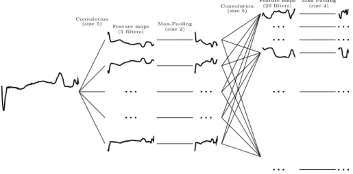
Model. Our CNN model, denoted t-leNet in the following, is a time-series
specific version of leNet model [11]. leNet has proved successful for image classi-fication. It is made of two convolutions layers, each followed by a sub-sampling step performed through max pooling. Finally, fully connected layers enable to match extracted features with class labels to be predicted. The convolutional part of our model is presented in Fig. 1: a first convolution with 5 filters of temporal span equal to 5 is used, followed by a max pooling of size 2. Then, a second convolution layer is made of 20 filters with the same time span as the previous ones and a final max pooling of size 4 is used.
Data augmentation. As presented above, CNN tend to suffer less from
overfitting than fully connected networks. However, it has been shown in the computer vision community that such models could still benefit from data aug-mentation methods [4]. This family of techniques aims at building synthetic data by transforming existing labelled samples so as to help the model learn the range of intra-class invariances one could observe. For example, when performing im-age classification, it is likely that flipping an imim-age will not change its class. In practice, such synthetic samples will be added to training sets so as to enrich
...
...
Feature maps (5 filters) Convolution (size 5)...
...
Max-Pooling (size 2)...
...
...
...
Feature maps (20 filters) Convolution (size 5)...
...
...
...
Max Pooling (size 4)Fig. 1: Convolutional part oft-leNet. On the left, raw time series are fed to the
network and features shown on the right are inputs for a supervised classifier.
them. In this section, we present the set of data augmentations we have used for time series.
A first method that is inspired from the computer vision community [8, 10] consists in extracting slices from time series and performing classification at the slice level. This method has been introduced for time series in [6]. At training, each slice extracted from a time series of classy is assigned the same class and
a classifier is learned using the slices. The size of the slice is a parameter of this method. At test time, each slice from a test time series is classified using the learned classifier and a majority vote is performed to decide a predicted label. This method is referred to as window slicing (WS) in the following.
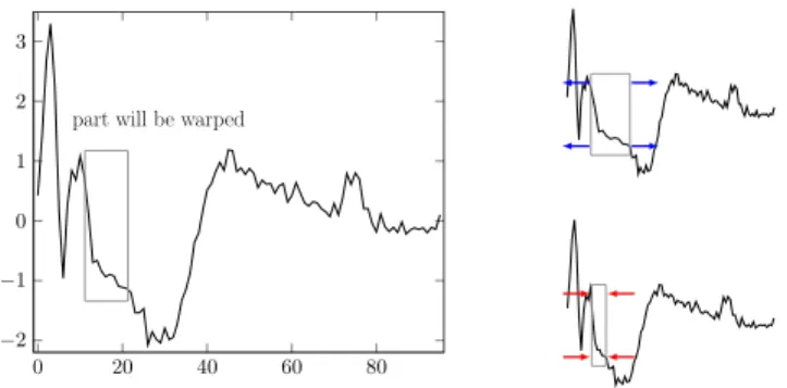
The last data augmentation technique we use is more time-series specific. It consists in warping a randomly selected slice of a time series by speeding it up or down, as shown in Fig. 2. The size of the original slice is a parameter of this method. Fig. 2 shows a time series from the “ECG200” dataset and corresponding transformed data. Note that this method generates input time series of different lengths. To deal with this issue, we performwindow slicing on transformed time series for all to have equal length. In this paper, we only consider warping ratios equal to 1
2 or2, but other ratios could be used and the optimal ratio could even
be fine tuned through cross-validation on the training set. In the following, this method will be referred to aswindow warping (WW).
Dataset mixing.An important finding that has enabled the efficient use of
huge amounts of data to learn deep models consists in pre-training the models. Indeed, it has been shown that the standard back-propagation procedure used to learn model parameters heavily suffers from the vanishing gradient phenomenon. To improve on this, pre-training each layer in an unsupervised manner (as an
0 20 40 60 80 2 1 0 1 2 3
part will be warped
Fig. 2: Example of thewindow warping data augmentation technique.
auto-encoder) enables to reach regions of the parameter space that are better seeds for the back-propagation procedure [3]. Building on this, we suggest to pre-train our model in a unsupervised manner using time series from various datasets. Once this pre-training step is done, convolution filters are kept and the supervised part of the model is trained separately for each dataset. This method is called dataset mixing (DM) in the following.
4 Experimental evaluation
All the experiments presented in this section are conducted on public datasets from the UCR archive [9] using thetorchframework [5]. When training neural networks, we use a learning rate of 0.01 with a decay of 0.005.
Impact of data augmentation.We first compare the efficiency of the data
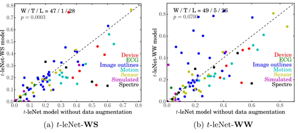
augmentation methods presented in Section 3. For this evaluation, we report dataset types as found in [1] that splits UCR datasets into 7 types: Device, ECG, Image outlines, Motion, Sensor, Simulated, and Spectro. Performance is studied through scatter plots of compared error rates and Win / Tie / Lose scores, and one-sided Wilcoxon signed rank test is used to assess statistical significance of observed differences (p-values are reported on the figures).
Fig. 3 indicates that bothWSandWWmethods help improve classification performance. For these experiments, the size of the slices forWSis set to90%
of the size of the original time series, while the size of the slices that are warped inWWis set to10%of the size of time series. Observed improvement forWW
cannot be considered significant at the 5% level because of error rate dispersion that is much higher than for theWSdata augmentation method. However, one interesting point is that for WW, we can derive a rule of thumb of when to use it: the method almost always improve performance except for datasets of
type Image outlines for which it should be avoided. Finally, when compared
to state-of-the-art methods, both WS and WW methods improve on basic distance-based method performance but are still dominated by PROP ensemble method (cf.Fig. 4).
0.0 0.1 0.2 0.3 0.4 0.5 0.6 0.7 0.8
t-leNet model without data augmentation
0.0 0.1 0.2 0.3 0.4 0.5 0.6 0.7 0.8 t -l eN et -W S m od el Device ECG Image outlines Motion Sensor Simulated Spectro W / T / L = 47 / 1 / 28 p= 0.0003 (a)t-leNet-WS 0.0 0.2 0.4 0.6 0.8
t-leNet model without data augmentation 0.0 0.2 0.4 0.6 0.8 t -l eN et -W W m od el Device ECG Image outlines Motion Sensor Simulated Spectro W / T / L = 49 / 5 / 26 p= 0.0700 (b)t-leNet-WW
Fig. 3: Impact of WSandWWon classification performance (both axes corre-spond to error rates). Win / Tie / Lose scores indicate that this kind of data augmentation tends to improve classification accuracy ("Win" means that the
y-axis method has lower error rate) and this difference can be considered
signif-icant at the 5% level fort-leNet-WS.
Dataset PROP MCNN t-leNet-+ FCWS DMt-leNet-+ SVMWS tDM-leNet-+ FCWS ChlorineCon. 0.360 0.203 0.188 0.129 0.203 ECG5000 – – 0.061 0.059 0.062 ECGFiveDays 0.178 0.000 0.001 0.002 0.002 FacesUCR 0.063 0.063 0.108 0.052 0.113 Gun_Point 0.007 0.000 0.007 0.006 0.000 Plane 0.000 – 0.048 0.010 0.038 wafer 0.003 0.002 0.003 0.002 0.002
Table 1: Error rates obtained using dataset mixing.
Dataset mixing and semi-supervised learning.We now turn our focus
on the impact of dataset mixing (DM). As presented above, this method con-sists in learning the convolutional part of our model in an unsupervised manner by mixing time series from several datasets. For this set of experiments, we have selected 7 datasets that share similar time series length. These datasets are listed in Table 1 that provides obtained error rates. Note thatWS method is used in these experiments. In this table, we report results obtained by using either a set of fully connected layers or a SVM to perform per-dataset supervised classifica-tion and one can observe that both methods obtain similar results. Second, our methods reach competitive performance when compared to PROP [12] that is an ensemble classifier considered as one of the most efficient baselines for time series classification these days, and MCNN [6], a CNN for time series.
0.0 0.1 0.2 0.3 0.4 0.5 0.6 0.7 0.8 1NN-DTW 0.0 0.1 0.2 0.3 0.4 0.5 0.6 0.7 0.8 t -l eN et -W S m od el Device ECG Image outlines Motion Sensor Simulated Spectro W / T / L = 56 / 4 / 16 p= 0.00002 (a)t-leNet-WSvs 1NN-DTW 0.0 0.1 0.2 0.3 0.4 0.5 0.6 0.7 0.8 PROP 0.0 0.1 0.2 0.3 0.4 0.5 0.6 0.7 0.8 t -l eN et -W S m od el Device ECG Image outlines Motion Sensor Simulated Spectro W / T / L = 13 / 5 / 23 p= 0.0554 (b)t-leNet-WSvs PROP 0.0 0.1 0.2 0.3 0.4 0.5 0.6 0.7 0.8 1NN-DTW 0.0 0.1 0.2 0.3 0.4 0.5 0.6 0.7 0.8 t -l eN et -W W m od el Device ECG Image outlines Motion Sensor Simulated Spectro W / T / L = 50 / 4 / 26 p= 0.0249 (c)t-leNet-WWvs 1NN-DTW 0.0 0.1 0.2 0.3 0.4 0.5 0.6 0.7 0.8 PROP 0.0 0.1 0.2 0.3 0.4 0.5 0.6 0.7 0.8 t -l eN et -W W m od el Device ECG Image outlines Motion Sensor Simulated Spectro W / T / L = 16 / 3 / 24 p= 0.0245 (d)t-leNet-WWvsPROP
Fig. 4: Comparison oft-leNet-WSandt-leNet-WWwith state-of-the-art
meth-ods (in each figure, both axes correspond to error rates).
5 Conclusion
In this paper, we have designed a Convolutional Neural Network for time se-ries classification. To improve the performance of this CNN when faced with small training sets, we propose two approaches to artificially increase the size of training sets. The first one is based on data-augmentation techniques. The second one consists in mixing different training sets and learning the network in a semi-supervised way. We show that these two approaches improve the overall classification performance. As a future work, we intend to improve the warping approach by considering more warping ratios and use more datasets to learn better feature extractors.
References
[1] Anthony Bagnall et al. “The Great Time Series Classification Bake Off: An Experimental Evaluation of Recently Proposed Algorithms. Extended version”. In:arXiv:1602.01711 (2016).
[2] Adeline Bailly et al. “Dense Bag-of-Temporal-SIFT-Words for Time Series Classification”. In: Lecture Notes in Artificial Intelligence (2016).
[3] Yoshua Bengio. “Learning deep architectures for AI”. In:Foundations and
trendsR in Machine Learning 2.1 (2009), pp. 1–127.
[4] K. Chatfield et al. “Return of the Devil in the Details: Delving Deep into Convolutional Nets”. In: British Machine Vision Conference. 2014. [5] Ronan Collobert, Koray Kavukcuoglu, and Clément Farabet. “Torch7: A
matlab-like environment for machine learning”. In:BigLearn, NIPS Work-shop. 2011.
[6] Zhicheng Cui, Wenlin Chen, and Yixin Chen. “Multi-Scale Convolutional Neural Networks for Time Series Classification”. In:arXiv:1603.06995 (2016). [7] Marco Cuturi. “Fast global alignment kernels”. In:Proceedings of the
In-ternational Conference on Machine Learning. 2011, pp. 929–936.
[8] Andrew G Howard. “Some improvements on deep convolutional neural network based image classification”. In:arXiv:1312.5402 (2013).
[9] Eamonn Keogh et al. The UCR Time Series Classification/Clustering
Homepage. http://www.cs.ucr.edu/~eamonn/time_series_data/.
2011.
[10] Alex Krizhevsky, Ilya Sutskever, and Geoffrey E Hinton. “Imagenet classi-fication with deep convolutional neural networks”. In:Advances in neural
information processing systems. 2012, pp. 1097–1105.
[11] Yann LeCun et al. “Gradient-based learning applied to document recogni-tion”. In:Proceedings of the IEEE 86.11 (1998), pp. 2278–2324.
[12] Jason Lines and Anthony Bagnall. “Time series classification with ensem-bles of elastic distance measures”. In:Data Mining and Knowledge Discov-ery 29.3 (2015), pp. 565–592.
[13] Chotirat Ann Ratanamahatana and Eamonn Keogh. “Three myths about dynamic time warping data mining”. In:Proceedings of SIAM International
Conference on Data Mining (SDM’05). SIAM. 2005, pp. 506–510.
[14] Patrick Schäfer. “The BOSS is concerned with time series classification in the presence of noise”. In:Data Mining and Knowledge Discovery 29.6 (2014), pp. 1505–1530.
[15] Pavel Senin and Sergey Malinchik. “SAX-VSM: Interpretable Time Series Classification Using SAX and Vector Space Model”. In:Proceedings of the
IEEE International Conference on Data Mining (2013), pp. 1175–1180.
[16] Jin Wang et al. “Bag-of-words representation for biomedical time series classification”. In: Biomedical Signal Processing and Control 8.6 (2013), pp. 634–644.
[17] Yi Zheng et al. “Time series classification using multi-channels deep convo-lutional neural networks”. In:Web-Age Information Management. Springer, 2014, pp. 298–310.