Decentralized Model Reference Adaptive Control Without Restriction on Subsystem Relative Degrees

[5] St. Kotsios, “Finite input/output representation of a class of Volterra polynomial systems,” Automatica, vol. 33, no. 2, pp. 257–262, 1997. [6] St. Kotsios and D. Lappas, “A description of 2-dimensional discrete

polynomial dynamics,” IMA J. Math. Control and Inform., vol. 13, pp. 409–428, 1996.

[7] L. Ljung, System Identification Theory for the User. Englewood Cliffs, NJ: Prentice-Hall, 1987.

[8] J. W. Rugh, Nonlinear System Theory. Baltimore, MD: Johns Hopkins Univ. Press, 1981.

Decentralized Model Reference Adaptive Control Without Restriction on Subsystem Relative Degrees

Changyun Wen and Yeng Chai Soh

Abstract—When the direct model reference adaptive control (MRAC)

scheme with first-order local estimators is employed to design totally decentralized controllers, the stability result can only be applied to a system with all of its nominal subsystem relative degrees less than or equal to two. In this paper, this restriction is relaxed and it is achieved by employing the parameter projection together with static normalization. To implement the local controllers, no a priori knowledge of the subsystem unmodeled dynamics and no information exchange between subsystems are required. Global stability is established for the closed-loop system and small in the mean tracking error is ensured. With this analysis, the class of interactions and subsystem unmodeled dynamics can be enlarged to include those having infinite memory.

Index Terms—Adaptive control, decentralized control, robustness,

sta-bility.

I. INTRODUCTION

Decentralized adaptive control is an important control scheme for large scale systems, and it has continued to receive a lot of attention from control researchers over the last few decades. However, only a limited number of stability results in this area are available due to the difficulties in the analysis of ignored interactions. The first batch of results were obtained based on the direct model reference adaptive control (MRAC) approach [1]–[3]. A strong assumption for these results is that relative degrees of all the nominal subsystem models should be less than or equal to two. The stability results using the indirect pole assignment design scheme were reported later in [4]–[6] where there is no restriction on the relative degrees of the nominal subsystem. Recently, efforts on relaxing the subsystem relative degrees in the case of employing the direct adaptive control scheme have been made by using some advanced adaptive strategies. The concept of high-order tuners in [7] was applied to achieve this in [8] and [9]. In this case, a local dynamic estimator with the subsystem relative degree as its order is designed to identify the unknown parameters of each subsystem. The integrator backstepping technique of [10] was also successfully utilized to reach a similar goal in [11]–[13]. To obtain the final control for each subsystem, a number of iterative design steps should be involved to calculate Manuscript received April 24, 1996; revised March 16, 1998. Recom-mended by Associate Editor, M. Krstic. This work was supported in part by NTU under the Applied Research Project Grant RP 23/92.

The authors are with the School of Electrical and Electronic Engineering, Nanyang Technological University, Singapore (e-mail: [email protected]).

Publisher Item Identifier S 0018-9286(99)04544-4.

some intermediate virtual control signals. As commented in [9], the unmodeled interactions must satisfy certain structural conditions when these advanced schemes are used.

However, for the conventional MRAC scheme, the problem of the relaxation of the subsystem relative degrees is still unsolved. Due to the simplicity of the conventional MRAC scheme, the solution to such a problem is of practical interest. In [14], Datta and Ioannou applied the normalization technique used in the single-loop robust adaptive controller design to achieve the required relaxation. But the proposed local normalizing signals require information from the other subsys-tems to bound the effects of interactions from these subsyssubsys-tems. Thus, only partially decentralized adaptive controllers can be designed. In this paper, the problem will be solved with totally decentralized controllers by employing the parameter projection together with a static normalization technique. Global stability is established for the closed-loop system and small in the mean tracking error is ensured. With our analysis, the class of interactions and subsystem unmodeled dynamics can be enlarged to include those having infinite memory.

The remaining part of the paper is organized as follows. Section II gives the class of systems to be controlled and Section III presents the decentralized controllers. The analysis of the closed-loop system and the main result are given in Section IV. Finally, the paper is concluded in Section V.

II. SYSTEM MODELS ANDASSUMPTIONS

In this paper, the class of interconnected systems considered con-sists ofm single-input/single-output subsystems. The ith subsystem is modeled as

yi(t) = Hi(D)ui(t) + Hi(D) m j=1

ijHij(D)[uj(t) + yj(t)]

+ m

j=1

ijHij(D)[uj(t) + yj(t)] + di(t) (1) fori; j = 1; 1 1 1 ; m, where yi; ui; and diare, respectively, the output, input, and disturbance of theith subsystem. In (1), Hi(D) = B (D)_{A (D)} and it is the reduced-order transfer function of subsystemi with

Ai(D) = Dn _{+ a}n 01

i Dn 01+ 1 1 1 + a0i Bi(D) = bm

i Dm + bm 01i Dm 01+ 1 1 1 + b0i

whereD denotes the differentiation operator, mi< ni; ij; ij are constants, and Hij(D) and Hij(D) denote the subsystem interactions if i 6= j and unmodeled dynamics if i = j.

Now, a reference model given below is chosen for theith sub-system

yim(t) = Wm(D)ri(t)i (2)

where Wm(D) = ki i_{mD (D)}1 and ri is an external reference input signal. Here, k_mi is a constant and Dim(D) is a monic Hurwitz polynomial of degree n3_i = ni 0 mi, i.e., Di_m(D) = Dn + di

n 01Dn 01+ 1 1 1 + di1D + di0. The control problem is to design totally decentralized controllers for plant (1) such that the closed-loop system is stable in the sense that all signals in the system are bounded for arbitrary boundedri and initial conditions, and the outputyi(t) follows the outputy_mi (t) of the model (2) as closely as possible. To solve the control problem, the following assumptions are made for the plant given in (1).

Assumption 2.1: A1) Bi(D) is Hurwitz.

A2) An upper bound forni, the nominal relative degree n3_i = ni0 mi of subsystemi, and the sign of the high frequency gain sgn(bm_i ) are known. Furthermore, the coefficients of Ai(D) and Bi(D) are inside a known compact convex region Ci.

A3) Hij (D) and Hij(D) are stable, and Hi(D) Hij(D) and

Hij(D) are strictly proper. A4) di(t) is bounded.

Remarks 2.1:

1) Note that there is no restriction on the nominal subsystem relative degreesn3_i; i = 1; 2; 1 1 1 ; m.

2) While modeling errors are assumed to satisfy A3) and A4), no a priori knowledge is required from them for the implemen-tation of the adaptive controllers given in the later sections. Assumption A2) also implies a known lower bound forjbm_i j. III. DESIGN OFROBUSTDECENTRALIZEDADAPTIVECONTROLLERS

For each subsystem, we define the following filtered variables: _!i;1= 3i!i;1+ qiyi; _!i;2= 3i!i;2+ qiui (3) where(3i; qi) is a controllable pair satisfying

(DI 0 3i)01_qi= 1

Fi(D)[Dn 02; 1 1 1 ; 1]T (4) withFi(D) as an arbitrary Hurwitz polynomial of order ni01. Both 3i and qi are chosen by users. Let

!T

i = !Ti;1; !Ti;2; yi : (5) Then the control is given as

ui= !Tii+ ci;0ri (6)

where_iT(t) = [_i;1T (t); _i;2T (t); i;3(t)] is a (2ni0 1)-dimensional control parameter vector and ci;0(t) is a feedforward parameter scalar. From [16], it can be shown that a desired parameter vector 3

i of i and a desired parameter c3i;0 of ci;0 exist, and they can be obtained when the nominal transfer functionHi(D) of the ith subsystem is known. WhenHi(D) is unknown, an adaptive law is required to update i and ci;0. To achieve this and to ensure the robustness of the adaptive controller in the presence of modeling errors including interactions, subsystem unmodeled dynamics, and external disturbances, we introduce parameter projection operation to the adaptive law. The adaptive law to tuneiandci;0is divided into the following two cases.

Case 1: bm_i = 1. In this case, ci;0 = 1 if k_mi is chosen to be one and _i= P i; 0 0_{1 + !}iei;1i_T i!i (7) where 0i = 0T_i > 0 ei;1= yi0 ym + T ii0 vi; i= Wmi(D)I !i vi= Wi m(D)iT!i (8) !T i = !Ti; iT; i(1) T ; 1 1 1 ; (n )_i T (9) andP denotes the projection operation defined in [17] or [18].

Case 2: bm_i is unknown. In this case, ci;0(t) is unknown and needs to be updated. The local adaptive law in this case is a modified version of that in [15] by changing the -modification and the normalizing signal appropriately as in Case 1.

Remarks 3.1:

1) As can be noted from (6)–(9), the normalization is static. Also the implementation of local adaptive controllers does not require any information exchange between subsystems and the a priori knowledge on subsystem unmodeled dynamics. 2) The results for the adaptive controller in Case 2 can be obtained

by following the similar analyses as in Case 1 and [15]. Thus we just focus our attention on Case 1 without any further elaboration on Case 2.

IV. STABILITY OF THEDECENTRALIZEDADAPTIVECONTROLSYSTEMS We need to establish the robustness of the local adaptive controllers in the presence of ignored interactions, unmodeled dynamics, and external disturbances. Before doing this, some preliminary analysis is required.

From (1)–(6), it can be shown that the ith subsystem can be expressed as

yi= Wm(D) !i iT~i+ ri + mi(t) (10) where

~i= i0 i3 (11)

mi(t) = i(t) + 1 + Wi

m(D)i;13 (DI 0 3i)01qi di (12) i(t) =

m j=1

1ij(D)[uj(t) + yj(t)] (13)

1ij(D) = W_m(D)i

ijHij(D) 1 0 3i;2(DI 0 3i)01qi

+ ijHij(D) 1 + W m(D)(i i;33 + i;13 (DI 0 3i)01qi : (14) Clearly,1ij(D) is strictly proper and stable from Assumption 2.1. From (12), we have the following result.

Lemma 4.1: The modeling errormi(t) in (12) satisfies jmi(t)j

m j=1

ij sup

0tk!j()k + d0 (15)

whereij andd0are some nonnegative constants.

Proof: LetVi(D) be an arbitrary Hurwitz polynomial defined as Vi(D) = Dn 02+ vi;n 03Dn 03+ 1 1 1 + vi;0

vTi = [1; vi;n 03; 1 1 1 ; vi;0]: Then

i(t) = m j=1

1ijFj_VjVj_Fj(uj+ yj) =

m j=1

1ijFj_Vj vjT(!j;1+ !j;2) : (16) Thus from the stability and properness of 1ijF_V , the result can be established from (16).

Remarks 4.1:

1) In the proof of Lemma 4.1, the effects of some exponentially decaying terms due to nonzero initial conditions have been absorbed by d0.

2) The constant ij indicates the strength of the interactions between subsystemsi and j when i 6= j, and the unmodeled dynamics of the ith subsystem are coupled to the nominal model wheni = j.

3) In terms of the bounding signals, the bound for the modeling error in (15) allows the effects of the unmodeled dynamics and interactions to have infinite memory, thus it is looser than those given in existing literature, such as [1] and [2]. The class of modeling errors considered can also be enlarged to include any nonlinear unmodeled dynamics satisfying (15).

Now, if sup_0tk!i()k = k!i(t)k and sup_0tk!j()k sup_0tk!i()k for all j 6= i and t > t0

i, then (15) becomes jmi(t)j k!i(t)k + d0; for allt t0_i (17) where is a nonnegative constant depending on ij.

From (17), some useful properties of the local estimators can be obtained.

In the remaining part of this section, we will usemk_i; k = 1; 1 1 1 ; 5 to denoteM_ik(D)mi where M_ik(D) is a vector containing proper stable transfer functions. Thus, mk_i(t); k = 1; 1 1 1 ; 5 also satisfy the same bounds as in (17) under the same conditions. Note that the constants and d0 in (17) have been made uniform for all i = 1; 2; 1 1 1 ; m and k = 1; 1 1 1 ; 5. Also in this section, all cj; j = 1; 2; 1 1 1 stand for generic constants.

We now derive an equation to describe the closed-loop system of theith loop. It can be shown that the plant in the ith loop has the following state representation:

_xi= Aixi+ biui+ m1

i(t); yi= hTixi+ m2i(t) (18) where(Ai; bi; hT_i) is a minimal state representation of Hi(D). Note thatDm2_i also satisfies (17) from the strict properness of Hij(D). Now the closed-loop system of theith loop can be described as

_xc

i= Acixci+ bci!Ti ~i+ bciri+ m1i(t) yi= hc

i Txci+ m2i(t)

(19) where Ac_i is a stable matrix satisfying (hci)T(DI 0 Aci)01bc_i = Wi

m(D) and xci = [xTi; !Ti;1; !i;2T ]T.

Let _iT = [_iT; _i(1) ; 1 1 1 ; (n 01)_i ]. Then _i(k) = DkW_mi(D) I !i; k = 0; 1; 1 1 1 ; n3

i 0 1 can have the following realization: _i= A i+ B !i

= A i+ B ;1!i;1+ B ;2!i;2+ B ;3hiTxi+ B ;3m2i(t) (20)

_i(k)= Cki (21)

whereCk= [0; 0; 1 1 1 ; I; 0 1 1 1 0] with zero being (2ni01)2(2ni01) block matrices andI an identity matrix at the (k +1)th position. A is a stable matrix satisfyingC_kT(DI 0 A )01B = DkWm(D)Ii and B = [B ;1; B ;2; B ;3].

Letxc_i = [xc_i ; _iT]T. Then we have _xc i= Acixci+ Bic!iT~i+ Bcir + m3i(t) (22) where Ac i = Ac i 0 B ;3hT i; B ;1; B ;2 A : (23) Bc

i is suitably augmented frombci. Clearly,Aci is a stable matrix. We now establish the relationship between !i and xc_i. It can be shown, by taking the modeling errormiinto account and following similar steps in the proof of [16, Th. C.1], that

kxi(t)k c1k!i(t)k + m4 i(t) : (24) Then xc i(t) = xTi(t); !Ti;1(t); !Ti;2(t); iT T c2k!i(t)k + m4 i(t) : (25) Also k!i(t)k = !T i;1(t); !i;2T (t); hci Txic(t) + m2i(t); iT; !Ti 0 di0I; 1 1 1 ; din 01I i T T c3 xc i(t) + m5i(t) : (26)

Before establishing the stability of the system, we now explore some properties of the estimator (7)–(9).

Lemma 4.2: The estimator (7)–(9), when applied to the plant given in (1), has the following properties.

1) _j!i(t)T~_i(t)j 1 + !T

i(t)!i(t)1=2

c4; fort 0: (27)

2) SupposeM0is a positive constant s.t.d0=M0 . If k!i(t)k > M0; sup_0tk!i()k = k!i(t)k and sup_0tk!j()k sup_0tk!i()k 8j 6= i and for all t > t0 with some t0 0, then t t j!i()T_~i()j 1 + !T i()!i() 1=2 d c5=0+ (1+ 2)(t 0 t0); fort t0 (28) where 1= (c6=0+ ); 2= (c6=0+ ) + c7 0 (29) and > 0; 0 2 (0; 1]. Proof: 1) !i(t)T_~i(t) 1 + !T i(t)!i(t) 1=2 k!i(t)k 1 + !T i(t)!i(t)1=2 j~i(t)j c1:

2) From (8) and (10), we have ei;1= T

i ~i+ mi(t): (30)

Then consider the following positive definite function: Vi= 1₂~T

i0i01~i: (31)

Using (7) and (30) gives _Vi 0 1₂ ~Tii 2 1 + !T i!i+ 12 (mi)2 1 + !T i!i: (32) From the assumption of the lemma and (17), we have

mi(t) 1 + !T

i!i 1=2

+ ; fort t0: (33)

Then fort t0, (32) becomes _Vi 0 1₂ ~iTi 2 1 + !T i!i + 12( + ) 2_{: (34)} Then t t T i ()~i() 2 1 + !T i!i d c8+ ( + ) 2_{(t 0 t0): (35)}

From (9), we can note that k k

(1+! ! ) ; k = 0; 1; 1 1 1 ; n3i are bounded. From (3), (6), (18), and (24), we can have

_!i 1 + !T i (t)!i(t) 1=2 c9( + ) + c10: (36) Now _i(n +1)= D Dn_Di0 Dim(D) m(D) I !i+ _!i = 0di₀(1) i 0 di1i(2)0 1 1 1 0 din 01i(n ) + _!i: (37) Therefore, similar bounds to (36) can be obtained for

_i(n +1) (1 + !T i(t)!i(t))1=2; d dt(1 + !iT!i)1=2 (1 + !T i !i)1=2

and d dt( ~T ii(k) (1 + !T i!i)1=2) k = 0; 1; 1 1 1 ; n3

i. Note that !i= nk=0diki(k). Thus if T

i(t)~i(t) 2 1 + !T

i(t)!i(t) 0 8t 2 [tj; tj+ 1tj];

and for sometj t0 (38) we can establish j!i(t)T_~i(t)j 1 + !T i(t)!i(t) 1=2 c11 0 + ( + ) c₀12; 8t 2 [tj; tj+ 1tj]: (39) Then (28) can be established from (35) and (39).

Remark 4.2: 1 can be made arbitrary small by reducing and 2 by makingM0 a sufficiently large number.M0is used here for the purpose of analysis only. It is not a design parameter.

From Lemma 4.2, (25), and (26), the stability of the system can be established under a special case. This is presented in the following lemma.

Lemma 4.3: Consider the decentralized adaptive system consisting of plant (1) and local adaptive controllers (6)–(9). Suppose that k!i(t0

i)k = M0 and for allt > t0i,sup0tk!i()k = k!i(t)k and sup_0tk!j()k k!i(t)k for all j 6= i. Then under Assumption 2.1, there exists a positive constant3₁such that for all

3

1 the closed-loop system ensures that sup

0tk!i()k M; 8i = 1; 2; 1 1 1 ; m (40) whereM = c12M0+ c13 with c12 1.

Proof: The solution of (22) is xc i(t) = eA (t0t )xci(t0) + t t e A (t0) _Bc i!iT()~i() + Bicri() + m3i() d:

AsAc_i is a stable matrix, there exist positive constantsc and such that

eA t ce0t: (41)

Suppose that the intermediate numberM0is also such thatkrik1 M0; 8i = 1; 2; 1 1 1 ; m. Then using (25), (26), (17), (27), and (41) gives k!i(t)k c3ce0(t0t ) _{c2 !i t0 + m}4 i t0 + c14 t t ce 0(t0) !Ti()~i() (1 + k!i()k2₎1=2k!i()k + _{(1 + k!i()k}!iT()~i()₂₎₁₌₂ +M0+ m3 i() d + m5i(t) c15M0+ c16 sup 0tk!i()k + c17 t t ce 0(t0)

2_{(1 + k!i()k}!iT()~i()₂₎₁₌₂k!i()k d + c18: (42) After some rearrangement of (42), the Bellman–Grownwall lemma can be applied. Then from Lemma 4.2, we can obtain that

k!i(t)k c19M0+ c20+ c21 sup

0tk!i()k (43)

for 3₁and 3where3₁and 3are sufficiently small constants satisfying

c22(3

1+ 32) < (44)

with3₁ depending on3₁ and 3₂ on 3.

Note that the right side of (43) is nondecreasing. Thus it can be rewritten as

sup

0tk!i()k c19M0+ c20+ c21 sup0tk!i()k: (45) Then from (45), we get

sup 0tk!i()k c19 1 0 c21M0+ c20 1 0 c21 (46)

if 3₁with the positive constant 3₁satisfyingc213₁< 1. Finally, the result is proved by letting 3₁ = minf31;31; g and c12= maxf c

10c ; 1g; c13= 10c c .

To establish the stability result for the general case, we explore the parameter estimator further, and this gives Lemma 4.4 as follows.

Lemma 4.4: If k!i(t)k > M0 for all t t0, and sup_0tk!j()k c12M0+ c13 for all t 2 [0; t1] and j = 1; 2 1 1 1 ; m, and sup0tk!i()k = k!i(t)k; sup0tk!j()k sup_0tk!i()k; 8j 6= i for all t t1with somet1 t0, then

t t j!i()T_~i()j 1 + !T i ()!i() 1=2 d c5=0+ (1+ 2) t 0 t0 ; fort t0 (47) where 1= [c6=0+ (c12+ c13)](c12+ c13): (48) Proof: By noting the condition of the lemma and using (17), we have

jmi(t)j

(1 + k!i(t)k2₎1=2 (c12+ c13) + ; 8t 2 [t0; t1]: (49) Fort t1, (33) becomes valid. Noting that c12 1, we can have (49) for allt t0. Then replacing (33) by (49) and by (c12+c13) in the proof of (28), we can establish (47).

Remark 4.3: Note that the property in the above lemma is quite similar to (28) in Lemma 4.2 except that is changed to (c12+c13). From Lemmas 4.2–4.4, we can establish our main stability result as follows.

Theorem 4.1: Consider the decentralized adaptive system con-sisting of plant (1) and local adaptive controllers (6)–(9). Under Assumption 2.1, there exists a constant3 such that for all 3, we have the following.

1) The closed-loop system is globally stable in the sense that all signals remain bounded8t and for all finite initial states, any boundedri, and arbitrarily bounded external disturbances. 2) The tracking errorei;1(t) = yi0 ym satisfies

t t e

2

i;1() d 1+ 2( + d0+ 0) t 0 t0i ; for allt0i 0 (50) where1; 2are positive constants.

Proof:

1) To show the boundedness of all the trajectories k!ik; i = 1; 2; 1 1 1 ; m, we consider a function k!(t)k defined as

k!(t)k = maxfk!1(t)k; k!2(t)k; 1 1 1 ; k!m(t)kg: (51) Clearly, the result is proved if k!(t)k is bounded. It can be noted thatk!(t)k is continuous and thus, starting with 0= 0

andk = 1; 2; 1 1 1 ; we can divide the time axis [0; 1) into the following two subsequences:

<0 k = [k01; sk] <+k = (sk; k) where <0k = ft j k!(t)k M0g and <+k = ft j k!(t)k > M0g (52) i.e., [0; 1) = 1 k=1 <0k [ 1 i=1 <+i : (53) Obviously, it suffices to prove thatk!(t)k is bounded in <+_k; 8k 1. This can be shown through induction. Thus we considert 2 <+₁ first. From the continuity ofk!(t)k; 9t12 <+

1 and ani 2 f1; 2; 1 1 1 ; mg such that sup0tk!()k = k!(t)k and k!(t)k = k!i(t)k for all t t1 and t 2 <+₁. Thussup_0tk!i()k = k!i(t)k and sup_0tk!j()k sup0tk!i() 8j 6= i, for all t t1 and t 2 <+1. Therefore, the conditions of Lemma 4.3 are satisfied for all t t1 and t 2 <+₁. Then from this lemma and noting that k!i(t0)k = k!(t0)k = M0, we can have, for allt t1and all 3₁, that sup 0tk!()k M (54) i.e., sup 0tk!i()k M; 8i = 1; 2; 1 1 1 ; m: (55) If the conditions of Lemma 4.2.2 or 4.3 are violated fort t1 and t 2 <+₁, the following two possibilities may occur to k!(t)k.

• Case 1: sup_0tk!()k = k!(t)k but k!(t)k = k!j(t)k; j 2 f1; 2; 1 1 1 ; mgni for all t > t1.

In this case, the condition that sup_0t k!j()k sup0tk!i()k; 8j 6= i cannot be satisfied. Thus Lemma 4.3 cannot be applied for t > t1. However, we now consider k!j(t)k. Clearly, there exists a t1_j such that k!j(t1

j)k = M0andk!j(t)k > M0for allt 2 [t1j; t1] <+1. Also in this case, we have, for t > t1

sup 0tk!j()k = k!j(t)k and sup 0tk!i()k sup0tk!j()k i 2 f1; 2; 1 1 1 ; mgnj: (56) Thus from (55) and (56), Lemma 4.4 can be applied tok!j(t)k fort t1_j. Then following the same steps as in the proof of Lemma 4.3 and applying Lemma 4.4 with “initial condition” k!j(t1

j)k = M0, we shall obtain (54) or (55) for all t t1 and all 3 where

3=_{c12+ c13}31 : (57)

• Case 2:sup_0tk!()k 6= k!(t)k for t 2 [t1; t2] <+₁ andsup_0tk!()k = k!(t)k for t > t2.

In this case, the condition thatsup_0tk!i()k = k!i()k cannot be satisfied fort t1. However, (54) or (55) automati-cally holds fort 2 [t1; t2]. If t2is infinite, the result is proved. For a finite t2and when t > t2, (54) or (55) can be shown under the condition (57) by following the same argument as in Case 1.

In this way, the boundedness ofk!(t)k is established over <+₁. Now assuming (54) or (55) holds8t 2 <+_k, it can be shown that, by following the proof of Lemma 4.3 and the above argument, (54) is also true8t 2 <+_k+1 from Lemma 4.4 with the “initial condition” k!i(tk+1

i )k = M0 fori 2 f1; 2; 1 1 1 ; g and tk+1i 2 <+k+1.

After establishing the boundedness ofk!i(t)k; 8i = 1; 2; 1 1 1 ; m, we can haveyi(t) and ui(t) bounded.

2) Once the boundedness of all the signals is established, then the tracking properties can be obtained by following similar analyses used in [15].

Remarks 4.4:

1) Note that trajectoryk!(t)k only has three possibilities. That is, it satisfies the condition of Lemmas 4.2.2 and 4.3, or Case 1, or Case 2.

2) In the stability analysis, we only need to take care of the subsystem in which the static normalizing signal has maximum magnitude among all the subsystems over a certain time interval and consider the situation that the magnitude exceeds a certain level, i.e.,k!(t)k M0. In this case, the locally normalized parameter estimation prediction error in the subsystem con-cerned becomes small and satisfies certain conditions specified in Lemmas 4.2 and 4.4. Also the inductive technique used and the division of time interval into two subsequences are crucial in the establishment of a uniform bound fork!(t)k over all subintervals.

V. CONCLUSION

In this paper, we have relaxed the subsystem relative degrees re-quirement imposed in model reference decentralized adaptive control using first-order local estimators. These local estimators are designed using parameter projection together with static normalization. In the implementation of the local controllers, no a priori knowledge of the subsystem unmodeled dynamics and no information exchanges between subsystems are required. It has been shown that global stability of the overall adaptive feedback system can be ensured, provided the strength of the interactions and subsystem unmodeled dynamics is sufficiently weak. For each subsystem, the effect of the modeling error, including interactions from other subsystems, can be allowed to have infinite memory. Despite the modeling error, we have shown that small in the mean tracking error can be achieved.

REFERENCES

[1] P. Ioannou and P. Kokotovic, “Decentralized adaptive control of in-terconnected systems with reduced-order models,” Automatica, vol. 21, pp. 401–412, 1985.

[2] P. Ioannou, “Decentralized adaptive control of interconnected systems,” IEEE Trans. Automat. Contr., vol. 31, pp. 291–298, 1986.

[3] D. T. Gavel and D. D. Siljak, “Decentralized adaptive control: Structural conditions for stability,” IEEE Trans. Automat. Contr., vol. 34, pp. 413–426, 1989.

[4] C. Wen and D. J. Hill, “Decentralized adaptive control of linear time varying systems,” in Proc. 11th World Congr. Automatic Control, Tallinn, 1990, vol. 4.

[5] , “Global boundedness of discrete-time adaptive control just using estimator projection,” Automatica, vol. 28, pp. 1143–1157, 1992. [6] C. Wen, “Indirect robust totally decentralized adaptive control of

continuous-time interconnected systems,” IEEE Trans. Automat. Contr., vol. 40, pp. 1122–1126, 1995.

[7] A. S. Morse, “A comparative study of normalized and unnormalized tuning errors in parameter-adaptive control,” in Proc. 30th IEEE Conf. Decision and Control, 1991.

[8] R. Ortega and A. Herrera, “A solution to the decentralized stabilization problem,” Syst. Contr. Lett., vol. 20, pp. 299–306, 1993.

[9] R. Ortega, “An energy amplification condition for decentralized adaptive stabilization,” IEEE Trans. Automat. Contr., vol. 41, pp. 285–288, 1996. [10] M. Krstic, I. Kanellakopoulos, and P. Kokotovic, “A new generation of adaptive controllers for linear systems,” IEEE Trans. Automat. Contr., vol. 39, pp. 738–752, 1994.

[11] C. Wen, “Decentralized adaptive regulation,” IEEE Trans. Automat. Contr., vol. 39, pp. 2163–2166, 1994.

[12] C. Wen and Y. C. Soh, “Decentralized adaptive control using integrator backstepping,” Automatica, vol. 33, pp. 1719–1724, 1997.

[13] S. Jain and F. Khorrami, “Global decentralized adaptive control of large scale nonlinear systems without strict matching,” in Proc. American Control Conf., 1995, pp. 2938–2942.

[14] A. Datta and P. Ioannou, “Decentralized adaptive control,” in Advances in Control and Dynamic Systems, C. T. Leondes, Ed. New York: Academic, 1992.

[15] P. A. Ioannou and K. S. Tsakalis, “A robust direct adaptive controller,” IEEE Trans. Automat. Contr., vol. 31, pp. 1033–1043, 1986.

[16] K. S. Narendra and A. M. Annaswamy, Stable Adaptive Systems. Englewood Cliffs, NJ: Prentice-Hall, 1989.

[17] S. M. Naik, P. R. Kumar, and B. E. Ydstie, “Robust continuous-time adaptive control by parameter projection,” IEEE Trans. Automat. Contr., vol. 37, pp. 182–197, 1992.

[18] J.-B. Pomet and L. Praly, “Adaptive nonlinear regulation: Estimation from the Lyapunov equation,” IEEE Trans. Automat. Contr., vol. 37, pp. 729–740, 1992.

[19] R. H. Middleton, G. C. Goodwin, D. J. Hill, and D. Q. Mayne, “Design issues in adaptive control,” IEEE Trans. Automat. Contr., vol. 33, pp. 50–58, 1988.

A Diagonal Recurrent Neural Network-Based Hybrid Direct Adaptive SPSA Control System

Xiao D. Ji and Babajide O. Familoni

Abstract—A direct adaptive simultaneous perturbation stochastic

ap-proximation (DA SPSA) control system with a diagonal recurrent neural network (DRNN) controller is proposed. The DA SPSA control system with DRNN has simpler architecture and parameter vector size that is smaller than a feedforward neural network (FNN) controller. The simulation results show that it has a faster convergence rate than FNN controller. It results in a steady-state error and is sensitive to SPSA coefficients and termination condition. For trajectory control purpose, a hybrid control system scheme with a conventional PID controller is proposed.

Index Terms— Diagonal recurrent neural network (DRNN), neural

network controller (NNC), simultaneous perturbation stochastic approx-imation (SPSA).

I. INTRODUCTION

Nonlinear adaptive control system design is a challenge in nonlin-ear control system theory. In general, one may use neural networks (NN) to identify and/or control unknown and/or uncertain nonlinear Manuscript received May 9, 1996; revised March 6, 1998. Recommended by Associate Editor, J. C. Spall.

The authors are with the Department of Electrical Engineering, The Univer-sity of Memphis, Memphis, TN 38152 USA (e-mail: [email protected]).

Publisher Item Identifier S 0018-9286(99)04545-6.

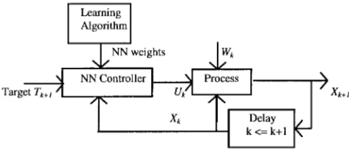
Fig. 1. Block diagram of the DA SPSA neural network-based control system. systems. To accomplish this, one needs to train (usually, offline) an inverse neural network as a controller. This is generally difficult since the system is unknown. An ideal scheme is a direct adaptive (DA) neural network control system. Spall described a generalized NN based on the simultaneous perturbation stochastic approximation (SPSA) approach to estimate the gradient of the performance function of an unknown nonlinear system [1]. Such a direct adaptive SPSA approach does not require any prior knowledge of the unknown system and does not need a separate training phase. An SPSA direct adaptive control system will converge to an optimal neural network parameter set, if it exists [3]. The NN-based SPSA approach as discussed in [2] and [3] uses a forward neural network (FNN) as the controller. The parameter vector size, in general, is large. For example, a network which contains four layers, two inputs, one out-put, with two hidden layers containing 20 and 10 nodes, respectively (denoted as @4_2;20;10;1), has 280 elements in the parameter vector. Other things being equal, its increased computational cost results in a slow performance measurement period (i.e., sampling period), and the performance measurement period is very important for a real-time control application.

As is well known, a recurrent neural network (RNN) has some advantages over FNN such as faster convergence, more accurate mapping ability, etc., but it is difficult to apply the gradient-descent method to update the neural network weights in RNN [4]. Ku et al. [5], [6] proposed the DRNN scheme that captures the dynamic behavior of a system and, since it is not fully connected, training is expected to be much faster than RNN. DRNN with time delay has RNN behavior but simple connections and is easy to use when applying the gradient-descent method. Therefore, in this paper, a diagonal recurrent neural network (DRNN) is employed in a DA SPSA control system. Simulation results are compared with those of the FNN SPSA scheme. These results also show that in general, after the SPSA process, the fixed DA SPSA neural network-based control results in a steady-state error because of the finite sample constraint of the SPSA approach. To improve the control performance, a conventional PID controller was employed to form a hybrid DA SPSA scheme. The proposed hybrid DA SPSA control system was examined by simulation and showed good performance.

II. SPSA BACKGROUND

Consider the problem of finding a root3of the gradient equation

g() @L()_@ = 0 (1)

for some differentiable cost function L : Rp ! R1. There are many methods for finding 3. In the case where L is observed in the presence of noise, an SA algorithm of the generic