Title
Efficient Estimation and Inference in Cointegrating
Regressions with Structural Change
Author(s)
Kurozumi, Eiji; Arai, Yoichi
Citation
Issue Date
2005-01
Type
Technical Report
Text Version
URL
http://hdl.handle.net/10086/16920
Discussion Paper #2004-09
Efficient Estimation and Inference in Cointegrating Regressions with Structural Change
Efficient Estimation and Inference in Cointegrating
Regressions with Structural Change
∗EIJI KUROZUMI†‡ YOICHI ARAI
Department of Economics Faculty of Economics Hitotsubashi University University of Tokyo
January, 2005
Abstract
This paper investigates an efficient estimation method for a cointegrating regression model with structural change. Our proposal is that we first estimate the break point by minimizing the sum of squared residuals and then, by replacing the break fraction with the estimated one, we estimate the regression model by the canonical cointegrating regression (CCR) method proposed by Park (1992). We show that the estimator of the
break fraction is consistent and of order faster thanT−1/2 and that the CCR estimator
with the estimated break fraction has the same asymptotic property as the estimator with the known break point. Simulation experiments show how the finite sample distri-bution gets close to the limiting distridistri-bution as the magnitude of the break and/or the sample size increases.
∗The discussion paper version of this paper might be updated occasionally. The latest version is available
at http://www.econ.hit-u.ac.jp/˜kurozumi/paper/efficient jan05.pdf.
†This paper was written while Eiji Kurozumi was a visiting scholar of Boston University.
‡Correspondence: Eiji Kurozumi, Department of Economics, Boston University, 270 Bay State Road,
1. Introduction
Cointegration is among the primary interests of a researcher who investigates the long-run relationship between economic variables. Single equation methods for testing cointegration or no cointegration have been developed by Engle and Granger (1987), Phillips and Ouliaris (1990), and Shin (1994) among others, while a system equation model is considered by Johansen (1988, 1991), Ahn and Reinsel (1990), L¨utkepohl and Saikkonen (2000), Saikkonen and L¨utkepohl (2000a, b), and papers in references of Hubrich, L¨utkepohl and Saikkonen (2001), who give a nice review of system methods.
It is often the case that data collected over relatively long time frames is used in the investigation of the long-run relationship, and the economic structure may change during the sample period. For a single or partial equation model, Campos, Ericsson and Hendry (1996) investigate the effect of structural change on cointegration tests, and Gregory and Hansen (1996a, b) propose tests for the null hypothesis of no cointegration with possibly one time structural break. Of importance is that the Gregory and Hansen’s test is robust to the existence of structural change but the test is not helpful in determining whether structural change has occurred or not. Thus, once the cointegrating relation with or without structural change is observed by the test, we need to test for structural change. Hansen (1992) proposes various tests for the parameter stability and Quintos and Phillips (1993) investigate the LM test for structural change, while Hao and Inder (1996) regard testing for structural change as a diagnostic test and develop the CUSUM test. The finite sample properties of Hansen’s (1992) tests are investigated by Gregory, Nason and Watt (1996) and Hao (1996), and they are generalized by Han (1996) to the exponential type tests as proposed by Andrews and Ploberger (1994) and Andrews, Lee and Ploberger (1996). Bai, Lumsdaine and Stock (1998) investigate testing for one time break and develop statistical inference about the estimator of the break point.
For a system equation model, tests of the cointegrating rank with a deterministic shift were developed by Saikkonen and L¨utkepohl (2000c), L¨utkepohl, Saikkonen and Trenkler (2003) for a known break point, while the unknown case is treated by Inoue (1999) and
L¨utkepohl, Saikkonen and Trenkler (2004). On the other hand, change in cointegrating vectors is considered by Quintos (1995) for known break points, while tests for structural change for unknown break points are proposed by Quintos (1997), Seo (1998) and Hansen and Johansen (1999). Hansen (2003) derives the limiting distribution of the maximum like-lihood estimator and proposes the likelike-lihood ratio test for parameter restrictions when the break point and the cointegrating rank are known. Unfortunately, tests for the cointegrat-ing rank with structural change assume the existence of structural change, whereas tests for structural change basically require the knowledge of the cointegrating rank. Additionally, to our best knowledge there is no test for the cointegrating rank with structural change in cointegrating vectors. Therefore, the system equation approach seems to be limited more or less when structural change in cointegrating vectors is incorporated in a model. For this reason, we consider a single equation model in this paper.
For a single equation model, suppose that we observe the cointegrating relation and structural change by using previously explained methods. If we know the date of structural change, we can estimate the model efficiently by the canonical cointegrating regression (CCR) method by Park (1992) and the fully modified regression (FMR) technique by Phillips and Hansen (1990) and Phillips (1995). However, we often encounter the case where we do not know the break date, and in this case the natural method for the estimation of the model is to first estimate the break point and then estimate the parameter in the model using the estimated break point. Bai, Lumsdaine and Stock (1998) show that the estimator of the parameter with the estimated break point has the same limiting distribution as the estimator with the known break point, assuming that the error term is independent of all leads and lags of the regressors. However, this assumption seems too restrictive for a cointegrating regression model because we often observe and commonly assume correlation between the error term and the regressors in a model. In this case, we cannot apply their result and are then required to find different methods to estimate the model with the unknown break point.
first, the error term is correlated with leads and lags of the regressors, and second that the break point is unknown. We propose to estimate the break point at first by minimizing the sum of squared residuals (SSR) and then, using the estimated break fraction, to estimate the model by the CCR method of Park (1992). We show that the estimator of the break fraction is consistent and of order faster thanT−1/2. Although this order may not be sharp, this is enough for us to derive the asymptotic distribution of the estimator of the parameter. Since the limiting distribution is shown to be a mixed normal, we can test parameter restrictions by constructing the Wald type test statistic, which converges to a chi-square distribution.
The structure of this paper is as follows. Section 2 explains the model and assumptions. In Section 3 we first derive the CCR estimator with the known break point. We then inves-tigate the asymptotic property of the estimator of the break fraction. Using this estimated break fraction, we estimate the regression model by the CCR method and show that the estimator of the parameter has the same limiting distribution as the CCR estimator with the known break point. Section 4 gives the finite sample property of the estimator. Section 5 concludes the paper.
2. A Model and Assumptions
Let us consider the following cointegrating regression model,
y1t = µ1+µ2ϕtτo +β10y2t+β20y2tϕtτo +v1t (1)
= b0xtτo +v1t,
for t = 1,· · ·, T, where {y1t} and {y2t} are one and m dimensional stochastic sequences,
ϕtτo is a step function such that ϕtτo = 0 for t ≤ [T τo] and ϕtτo = 1 for t > [T τo],
b = [µ1, µ2, β10, β20]0, and xtτo = [1, ϕtτo, y02t, y02tϕtτo]0. Let vt = [v1t, v20t]0 where v2t = 4y2t, and define its long-run variance as Ω = limT T−1E[VTVT0] whereVT =
PT t=1vt. We partition Ω conformably withvtas Ω = " ω11 ω021 ω21 Ω22 # .
We also define Σ = lim T→∞T −1XT t=1 E[vtvt0], Λ = lim T→∞T −1TX−1 j=1 TX−j t=1 E[vtvt0+j], Γ = Σ + Λ = " γ11 γ120 γ21 Γ22 # = " γ0 1 Γ02 # ,
where Γ is partitioned conformably withvt.
We employ the following set of assumptions throughout the paper.
Assumption 1 (a)y0 is a fixed or a random vector withE[y0]<∞and independent ofT. (b) {vt} is mean-zero and strong mixing with mixing coefficients of size −pα/(p−α) and
E|vt|<∞ for some p > α >5/2.
(c) The matrixΩ exists with finite elements, Ω>0, ω11>0, and Ω22>0.
(d) The break fractionτo is constant and τo∈ T = [τ ,τ¯]for known 0< τ <τ <¯ 1.
(e)β2=β2T =T−1/2β2o where β2o is a fixed vector.
Assumption (a) gives the initial value condition such thaty0 does not affect the
asymp-totic theory derived in the following sections. Assumptions (b) and (c) ensure that the functional central limit theorem (FCLT) holds for the partial sum process of{vt}, so that
T−1/2 [XT r] t=1 vt⇒B(r) = " B1(r) B2(r) # 1 m ,
whereB(r) is an (m+ 1) dimensional Brownian motion with the variance matrix Ω and ⇒
signifies weak convergence of the associated probability measures. The positive definiteness of Ω22 excludes the case where y2t is cointegrated. Assumption (d) is standard for a struc-tural break model. Assumption (e) is used to derive the convergence rate of the estimator of the break fraction. Strictly speaking, this assumption is not necessary for our asymptotic theory because we will not derive the limiting distribution of ˆτ, the estimator of the break fraction. However, as will be discussed in the next section, if we assume thatβ2 is fixed, the
asymptotic property of ˆτ will be determined only byy2t and a constant term will no longer play an important role for estimation ofτ. (e) is assumed so that both a constant and the I(1) regressors are effective in the estimation of the break point.
3. The CCR Estimator with Structural Change
Our strategy for estimation is that we first obtain the estimate of the break point by mini-mizing the SSR and then estimate (1) by the CCR method using the estimated break point. We will show that the CCR estimator with the estimated break point has the same limiting distribution as the CCR estimator with the known break point. Note that, although the following explanation proceeds based on the CCR method, we can easily apply our result to the fully modified regression (FMR) technique by Phillips and Hansen (1990) and Phillips (1995). The difference between the CCR and the FMR methods resides in how to correct serial correlations. See Phillips and Hansen (1990) and Park (1992) for details.
3.1. The CCR method with a known break point
First, we briefly explain the CCR method for a known break point. It consists of two separate step estimations. The first step is to estimate (1) by OLS regression. Let ˆbτo =
[ˆµ1τo,µˆ2τo,βˆ01τo,βˆ
0
2τo] be the OLS estimator of b and ˆv1tτo be the OLS residual. Using ˆbτo
and ˆv1tτo we construct variablesy1∗tτo and y
∗ 2tτo as y∗1tτo =y1t−( ˆβ10τoΓˆ 0 2τoΣˆ −1 τo + ˆβ 0 2τoΓˆ 0 2τoΣˆ −1 τo ϕtτo+[0,ωˆ021τoΩˆ −1 22τo])ˆvtτo, y2∗tτo =y2t−Γˆ 0 2τoΣˆ −1 τo vˆtτo,
where ˆvtτo = [ˆv1tτo,4y20t]0 and ˆΓ2τo, ˆΣτo, ˆω21τo, and ˆΩ22τo are consistent estimators of Γ2,
Σ,ω21, and Ω22that are defined below. Then, the CCR estimator is obtained by regressing
y∗ 1tτo ony ∗ 2tτo, y1∗tτo =b∗0τox∗tτo +e∗tτo, (2) where x∗ tτo = [1, ϕtτo, y2∗0tτo, y ∗0
2tτoϕtτo]0. We denote the CCR estimator and the estimated
residual as ˆb∗
τo and ˆe
∗
tτo.
The long-run matrices are estimated by ˆ Στo =T−1 T X t=1 ˆ vtτoˆv0tτo, Λˆτo =T−1 ` X j=1 k(j/`) TX−j t=1 ˆ vtτoˆvt+jτo, ˆ Γτo = ˆΣτo + ˆΛτo, Ωˆτo = ˆΣτo + ˆΛτo+ ˆΛ0τo,
Assumption 2 (a) k(·) is a continuous and even faction with |k(·)| ≤ 1, k(0) = 1 and R∞
−∞k2(x)dx <∞.
(b)` goes to infinity as n→ ∞ and `=o(T1/2).
Assumption 2 suffices to guarantee the consistency of ˆΛτo, ˆΓτo, and ˆΩτo, and many well
known kernels such as the Bartlett and the quadratic spectral kernels satisfy this assumption. See, for example, Andrews (1991).
The asymptotic distribution of ˆb∗
τo is given by the following proposition, which can be
proved in exactly the same way as Park (1992). Since this is the case, we omit the proof.
Proposition 1 Let Assumptions 1 (a)-(d) and Assumption 2 hold. Then, asT → ∞,
DT(ˆb∗τo−b) d −→ µZ 1 0 Xτo(r)Xτo(r) 0dr ¶−1Z 1 0 Xτo(r)dB1·2(r), (3) where DT = diag{T1/2, T1/2, T Im, T Im}, Xτo(r) = [1, ϕτo(r), B2(r)0, B2(r)0ϕτo(r)]0, ϕτo(r)
is a step function on[0,1]such thatϕτo(r) = 1{r≥τo}with1{·}being an indicator function,
andB1·2(r) =B1(r)−ω0
21Ω−221B2(r).
As discussed in Park (1992), the Wald test statistic based on the CCR estimator has an asymptotic chi-square distribution because (3) is a mixed normal distribution. For example, let us consider the general hypothesis of the form
H0 : g(b) = 0
where g(·) is a continuously differentiable q dimensional vector. Assume that G(b) =
∂g(b)/∂b0 is of rank q. Then, from Proposition 1, we can see that
WT(ˆb∗τo) = g(ˆb∗τo)0 ωˆ ∗ 1·2τoG(ˆb ∗ τo) Ã T X t=1 x∗tτox∗0tτo !−1 G(ˆb∗0τo) −1 g(ˆb∗τo) (4) d −→ χ2q, where ˆω∗
1·2τo is a consistent estimator of the long-run varianceω1·2, which can be constructed
3.2. The CCR method with an unknown break point
Regressions (1) and (2) are infeasible in practice because we do not know the true break point. A feasible method is that we first estimate the break point and then estimate the model using the estimated break point by the CCR method.
In the framework of cointegrating regressions, Bai, Lumsdaine and Stock (1998) inves-tigated the quasi-maximum likelihood estimator of the break point and they derived the limiting distribution of the estimator. One of the important assumptions in their paper is that the disturbance v1t must be independent of the regressors for all leads and lags (Assumption 3.2 in Bai, Lumsdaine and Stock, 1998). However, it is apparent that this assumption is not satisfied in our model, and we cannot apply their result. Therefore, we must investigate the asymptotic behavior of the estimator of the break point under general assumptions.
Let us consider a feasible version of the regression (1)
y1t=b0xtτ +v1tτ, (5)
whereτ ∈ T and v1tτ =v1t−b0(x
tτ −xtτo). Let ˆbτ and ˆv1tτ be the OLS estimator ofb and
the regression residual. The estimator of the break point is obtained by minimizing the sum of squared residuals in (5), or equivalently, the estimator of the break fraction is given by
ˆ
τ = arg inf
τ∈T ST(τ),
whereST(τ) =T−1
PT
t=1vˆ12tτ. We first give the consistency of ˆτ by the following proposition.
Proposition 2 Let Assumptions 1 (a)-(e) hold. Then, τˆ−→p τo.
Assumption 1 (e) implies that the magnitude of the break for y2t shrinks to zero as
T goes to infinity and is of order T−1/2. It is not difficult to see that Proposition 2 holds
without Assumption 1 (e). The reason we assume Assumption 1 (e) is that, ifβ2 is supposed
to be fixed,y2t asymptotically dominates the other terms in the objective function and the asymptotic property of ˆτ will be determined only by the behavior ofy2t. Assumption 1 (e)
is supposed so that both a constant andy2t have the same importance for determining the asymptotic behavior of the estimator. See also Bai, Lumsdaine and Stock (1998).
Once the consistency of ˆτ is obtained, we can restrict the parameter space of τ to only the vicinity of τo that shrinks to τo. Details are given in the appendix. By considering the shrinking parameter space, we can prove the next proposition.
Proposition 3 Let Assumptions 1 (a)-(e) hold. Then, T1/2(ˆτ−τ
o)−→p 0.
Proposition 3 implies that ˆτ converges in probability to τo of order faster than T−1/2. This convergence rate is slower than that obtained by Bai, Lumsdaine and Stock (1998) and the result in Proposition 3 may not be sharp. However, our purpose is not to derive the limiting distribution of the estimator of the break fraction but to obtain a feasible method of statistical inference about regression coefficients when the break point is unknown. The convergence rate given by Proposition 3 is enough for us to obtain such a feasible method and we do not pursue a sharp rate of ˆτ under general assumptions.
To construct the CCR estimator we need the estimators of the long-run variances. In exactly the same way as the known break point case, we construct ˆΣˆτ, ˆΛτˆ, ˆΓˆτ, and ˆΩτˆ by
replacing ˆvtτo by ˆvtτˆ = [ˆv1tτˆ,4y20t]0. The following proposition shows that these estimators are consistent.
Proposition 4 Let Assumptions 1 (a)-(e) and Assumption 2 hold. Then,Σˆτˆ, Λˆτˆ,Γˆˆτ, and ˆ
Ωτˆ converge in probability to Σ,Λ, Γ, and Ω, respectively.
We are now in a position to construct the CCR estimator using the estimated break point, ˆτ. Let y1∗tτˆ and y∗2tτˆ be defined in the same way as y1∗tτo and y2∗tτo using ˆτ. The feasible CCR estimator, ˆbτˆ, is obtained by regressing y∗
1tˆτ and y2∗tτˆ. The following is the
main theorem in this paper.
Theorem 1 Let Assumptions 1 (a)-(e) and Assumption 2 hold. Then,
DT(ˆb∗τˆ−ˆb∗τo)
p
Theorem 1 implies that the CCR estimator with the estimated break point has the same limiting distribution as the estimator with the known break point. Then, even if we construct the Wald test statistic forH0 using the feasible CCR estimator, it converges in
distribution to a chi-square distribution withq degrees of freedom, that is,
WT(ˆb∗ˆτ) = g(ˆb∗τˆ)0 ωˆ ∗ 1·2ˆτG(ˆb∗ˆτ) à T X t=1 x∗tˆτx∗0tτˆ !−1 G(ˆb∗0ˆτ) −1 g(ˆb∗τˆ) d −→ χ2q.
To conclude this section, we consider the extension of the model (1) in several directions. For example, we may be interested in a partial change of the parameters. In this case, we can easily see that all of the results in the paper are established in exactly the same manner. We may also want to include a linear trend as a regressor,
y1t=µ1+µ2ϕtτo +d1t+d2tϕtτo+β10y2t+β20y2tϕtτo +v1t.
Again, the propositions and the theorem can be shown to hold for this model. In this case,
DT is defined as DT = diag{T1/2, T1/2, T3/2, T3/2, T Im, T Im} and the definition of Xτo
in (3) should be changed appropriately. Seasonal constants may be of particular interest for some researchers and they may be included. In any case, although the expression (3) of the limiting distribution should be changed, the Wald statistic still has an asymptotic chi-square distribution and we can make statistical inferences about regression coefficients.
4. Finite sample evidence
In this section, we investigate finite sample properties of the feasible CCR estimator and the Wald test statistic proposed in the previous section. We consider the following data generating process:
y1t=µ1+µ2ϕtτo +β1y2t+β2y2tϕtτo +v1t, (6)
vt=Avt−1+εt,
where y2t is a one dimensional unit root process, vt = [v1t,4y2t]0, A = diag{a, a}, and
300 or 500. The break fractionτo is set to be 0.5 for all experiments. The values ofµ2 and
β2 are selected as follows. First, we regardd=µ2+β2× {V ar(y2t)}1/2 as a measure of the
magnitude of the change. We also note that variation iny1,t+1 given y1,t is v2,t+1+v1,t+1
for all t if structural change does not occur at t and its standard deviation is given by
{V ar(v2,t+1+v1,t+1)}1/2= 21/2 when vtis an i.i.d. sequence. We choose µ2 and β2 so that
the magnitude of the break,d, becomes approximately equal tos×21/2 fors= 0.5, 1, 2, or
3 att=T τo+ 1. According to this rule, we set{µ2, β2}={0.35,0.05},{0.7,0.1},{1.4,0.2},
and{2.1,0.3}, which correspond to the cases where T = 100 ands= 0.5, 1, 2, and 3. The same sets of values are also used forT = 300 and 500 to see the effect of the sample size on the finite sample property.
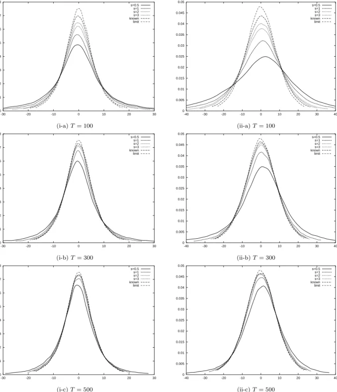
First, we see the finite sample distributions of the estimates ofβ1 andβ2. Figure 1 shows the probability density functions (pdf) ofT( ˆβ1−β1) andT( ˆβ2−β2) fora= 0, each of which
is drawn based on 100,000 replications. We can see that the pdf has fatter tails for each case when the magnitude of the break is smaller. The finite sample distribution approaches the limiting distribution as the magnitude of the break becomes larger, and the pdf with the known break point is closest to the limiting distribution. As expected, the finite sample distribution approaches the limiting distribution when the sample size is large. We can also see that the pdf of ˆβ2 is not as close to the limiting distribution as the pdf of ˆβ1. This is
becauseβ1 is estimated using the whole sample period, whileβ2 is estimated using only the
observations after the break point. As a whole, more than 300 observations are required to approximate the finite sample distribution by the limiting one when the magnitude of the change is very small (s= 0.5).
The above property is preserved when a = 0.6 and a = −0.6, but the finite sample distribution is slightly closer to the limiting one fora= 0.6 compared with the case when
a= 0, while the difference between the finite and the limiting distributions is slightly larger when a = −0.6 than the case when a = 0 (we do not draw the pdfs when a 6= 0 to save space).
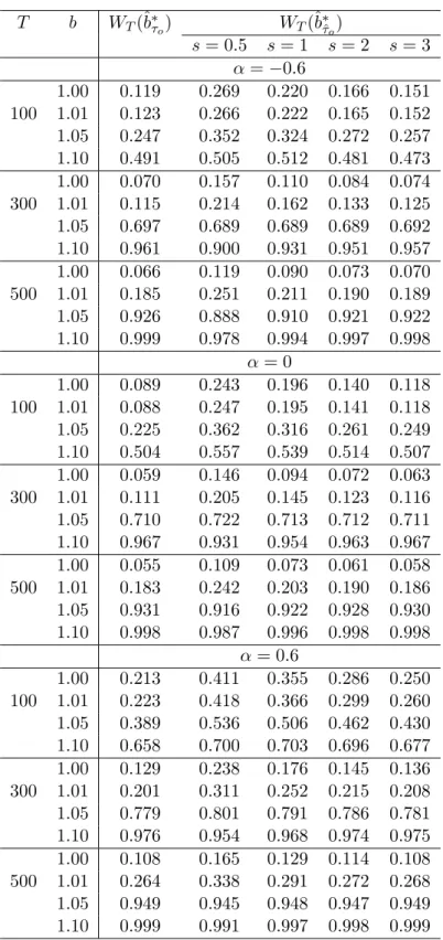
hypothesis of H0 : β1 =b and construct the test statistic. We set b= 1 to see the size of
the test, while it is set to be 1.01, 1.05, and 1.1 to investigate the power of the test. The level of significance is 0.05 and the number of replications is 5,000 in all experiments.
Table 1 summarizes the results of the simulations. When the break point is known, the size of the test is close to the nominal one whena= 0, but the test suffers from size distortion whena= 0.6. As expected from Figure 1, the size of the Wald statistic with the estimated break point approaches the known break point case as the magnitude of the break is larger. Regarding power, the test becomes more powerful when |b1o −1| increases. Although we must be cautious of the comparison of the power for different settings of parameters, the power property of the test does not seem to depend significantly on the value ofa.
We also investigate the size and power of the Wald test forb2. The performance of the
test under the null hypothesis is similar to the test ofb1, but the test of b2 is less powerful than that ofb1 (we do not report this result to save space).
5. Conclusion
In this paper we proposed to estimate the cointegrating regression model with structural change by the CCR estimation technique with the break point replaced by the estimated one. We first estimated the break fraction by minimizing the sum of squared residuals, and this estimator was shown to converge in probability to the true break fraction at a rate faster thanT1/2. We found that the feasible CCR estimator converges in distribution to a mixed normal distribution, so that the Wald test statistic based on it is asymptotically chi-square distributed. By Monte Carlo simulations, we showed that the finite sample distribution of the estimator approaches the limiting distribution as the magnitude of the break and/or the sample size becomes larger.
It might be possible to obtain an efficient estimator by other methods such as the dy-namic OLS (DOLS) method used by Saikkonen (1991) and Stock and Watson (1993), which estimates the model by adding leads and lags of the first differences of the I(1) regres-sors, where the lag length goes to infinity as T → ∞. Since the number of the regressors
changes depending on the sample size, much would be required to obtain the results given by Propositions 2 and 3.
References
[1] Ahn, S. K. and G. C. Reinsel (1990) Estimation for partially nonstationary multivariate autoregressive models. Journal of the American Statistical Association85, 813-823.
[2] Andrews, D. W. K. (1991) Heteroskedasticity and autocorrelation consistent covariance matrix estimation, Econometrica59, 817-858.
[3] Andrews, D. W. K., I. Lee and W. Ploberger (1996) Optimal changepoint tests for normal linear regression.Journal of Econometrics 70, 9-38.
[4] Andrews, D. W. K. and W. Ploberger (1994) Optimal tests when a nuisance parameter is present only under the alternative,Econometrica 62, 1383-1414.
[5] Bai, J., R. L. Lumsdaine and J. H. Stock (1998) Testing for and dating common breaks in multivariate time series. Review of Economic Studies65, 395-432.
[6] Campos, J., N. R. Ericsson and D. F. Hendry (1996) Cointegration tests in the presence of structural breaks.Journal of Econometrics 70, 187-220.
[7] Engle, R. F. and C. W. J. Granger (1987) Co-integration and error correction: Repre-sentation, estimation, and testing. Econometrica55, 251-276.
[8] Gregory, A. W. and B. E. Hansen (1996a) Residual-based tests for cointegration in models with regime shifts.Journal of Econometrics70, 99-126.
[9] Gregory, A. W. and B. E. Hansen (1996b) Tests for cointegration in models with regime and trend shifts. Oxford Bulletin of Economics and Statistics58, 555-560.
[10] Gregory, A. W., J. M. Nason and D. G. Watt (1996) Testing for structural breaks in cointegrated relationships. Journal of Econometrics71, 321-341.
[11] Hansen, B. E. (1992) Tests for parameter instability in regressions with I(1) processes.
[12] Hansen, P. R. (2003) Structural changes in the cointegrated vector autoregressive model.Journal of Econometrics114, 261-295.
[13] Hansen, H. and S. Johansen (1999) Some tests for parameter constancy in cointegrated VAR-models. Econometrics Journal 2, 306-333.
[14] Hao, K. (1996) Testing for structural changes in cointegrated regression models: Some comparisons and generalizations.Econometric Reviews 15, 401-429.
[15] Hao, K. and B. Inder(1996) Diagnostic test for structural change in cointegrated re-gression models. Economics Letters50, 179-187.
[16] Hubrich, K., H. L¨utkepohl and P. Saikkonen (2001) A review of systems cointegrating tests. Econometric Reviews20, 247-318.
[17] Inoue, A. (1999) Tests of cointegrating rank with a trend-break.Journal of Economet-rics 90, 215-237.
[18] Johansen, S. (1988) Statistical analysis of cointegration vectors. Journal of Economic Dynamics and Control12, 231-254.
[19] Johansen, S. (1991) Estimation and hypothesis testing of cointegration vectors in Gaus-sian vector autoregressive models.Econometrica 59, 1551-1580.
[20] L¨utkepohl, H. and P. Saikkonen (2000) Testing for the cointegrating rank of a VAR process with a time trend. Journal of Econometrics95, 177-198.
[21] L¨utkepohl, H., P. Saikkonen and C. Trenkler (2003) Comparison of tests for the coin-tegrating rank of a VAR process with a structural shift. Journal of Econometrics113, 201-229.
[22] L¨utkepohl, H., P. Saikkonen and C. Trenkler (2004) Testing for the cointegrating rank of a VAR process with level shift at unknown time. Econometrica72, 647-662.
[24] Park, J. Y., and P. C. B. Phillips (1988) Statistical inference in regressions with inte-grated processes: Part 1.Econometric Theory 4, 468-497.
[25] Phillips, P. C. B. (1995) Fully modified least squares and vector autoregression. Econo-metrica 63, 1023-1078.
[26] Phillips, P. C. B., and B. E. Hansen (1990) Statistical inference in instrumental variables regression with I(1) processes. Review of Economic Studies57, 99-125.
[27] Phillips, P. C. B. and S. Ouliaris (1990) Asymptotic properties of residual based tests for cointegration.Econometrica 58, 165-193.
[28] Quintos, C. E. (1995) Sustainability of the deficit process with structural shifts.Journal of Business and Economic Statistics 13, 409-417.
[29] Quintos, C. E. (1997) Stability tests in error correction models.Journal of Econometrics
82, 289-315.
[30] Quintos, C. E. and P. C. B. Phillips (1993) Parameter constancy in cointegrating re-gressions.Empirical Economics 18, 675-706.
[31] Saikkonen, P. (1991) Asymptotically Efficient Estimation of Cointegration Regressions.
Econometric Theory 7, 1-21.
[32] Saikkonen, P. and H. L¨utkepohl (2000a) Testing for the cointegrating rank of a VAR process with a intercept.Econometric Theory 16, 373-406.
[33] Saikkonen, P. and H. L¨utkepohl (2000b) Trend adjustment prior to testing for the cointegrating rank of a vector autoregressive process.Journal of Time Series Analysis
21, 435-456.
[34] Saikkonen, P. and H. L¨utkepohl (2000c) Testing for the cointegrating rank of a VAR process with structural shifts.Journal of Business and Economic Statistics18, 451-464.
[35] Seo, B. (1998) Tests for structural change in cointegrated systems.Econometric Theory
14, 222-259.
[36] Shin, Y. (1994) A residual- based test of the null of cointegration against the alternative of no cointegration. Econometric Theory 10, 91-115.
[37] Silverman, B. W. (1986)Density Estimation for Statistics and Data Analysis. Chapman and Hall, London.
[38] Stock, J. H. and M. W. Watson (1993) A Simple Estimator of Cointegrating Vectors in Higher Order Integrated Systems. Econometrica61, 783-820.
Appendix
Without loss of generality we shall assume thatT τo and Tτˆare integers in this appendix.
Proof of Proposition 2: We need to show that P(|τˆ−τo| > ε) → 0 for every ε > 0. Noting that P(|τˆ−τo|> ε) = P Ã inf τ∈T \δ(ε)ST(τ)<τ∈infδ(ε)ST(τ) ! ≤ P Ã inf τ∈T \δ(ε)ST(τ)< ST(τo) ! , (7)
where δ(ε) = {τ : |τ −τo| < ε}, it is sufficient to show that the right-hand side in (7) converges to zero.
The following lemma gives the limiting distribution of the OLS estimator of b.
Lemma 1 When τ =τo, DT(ˆbτo −b)⇒ µZ 1 0 Xτo(r)X 0 τo(r)dr ¶−1µZ 1 0 Xτo(r)dB2(r) + [0,0, γ 0 21,(1−τo)γ021]0 ¶ ≡ητo, (8) while forτ 6=τo, T−1/2DT(ˆbτ−b)⇒ − µZ 1 0 Xτ(r)X 0 τ(r)dr ¶−1Z 1 0 Xτ(r)∇X 0 2τ(r)dr b2≡ητ, (9) where ∇X2τ(r) = [ϕτ(r)−ϕτo(r), B02(r)(ϕτ(r)−ϕτo(r))]0 and b2 = [µ2, β20o]0.
Proof of Lemma 1: (8) is obtained in the same way as Park and Phillips (1988). To prove (9), note that T−1/2DT(ˆbτ −b) = Ã D−T1 T X t=1 xtτx0tτD−T1 !−1Ã T−1/2D−T1 T X t=1 xtτv1tτ ! . (10)
Using the FCLT and the continuous mapping theorem (CMT), we haveDT−1PTt=1xtτx0tτD−T1 ⇒
R1
0 Xτ(r)Xτ0(r)dr uniformly over τ. On the other hand, the term in the last parentheses on the right hand side of (10) becomes
T−1/2D−T1
T
X
t=1
= " T−1 T X t=1 v1tτ, T−1 T X t=1 v1tτϕtτ, T−3/2 T X t=1 y20tv1tτ, T−3/2 T X t=1 y20tv1tτϕtτ #0 . (11) Since v1tτ =v1t−b02∇x2tτ, where∇x2tτ = [ϕtτ −ϕtτo, T−1/2y02t(ϕtτ −ϕtτo)]0, we have T−1 [XT r] t=1 v1tτ = T−1 [T r] X t=1 v1t−b02T−1 [T r] X t=1 ∇x2tτ (12) ⇒ −b02 Z r 0 ∇X2τ(s)ds, T−3/2 [XT r] t=1 y2tv1tτ = T−3/2 [XT r] t=1 y2tv1t−T−3/2 [T r] X t=1 y2t∇x02tτb2 (13) ⇒ − Z r 0 B2(s)∇X 0 2τ(s)ds b2,
for 0≤r≤1. Using these results, we obtain (9).2
Next, we investigate the asymptotic behavior of ST(τ)−ST(τo) on τ ∈ T \δ(ε). We expandST(τ) andST(τo) as ST(τ) = T−1 T X t=1 (y1t−ˆb0τxtτ)2 = T−1 T X t=1 (b0xtτo +v1t−ˆbτ0xtτ +b0xtτ −b0xtτ)2 = T−1 T X t=1 {v1t−(ˆbτ −b)0DTDT−1xtτ −b02∇x2tτ}2 = T−1 T X t=1 v21t+T−1/2(ˆbτ −b)0DT Ã DT−1 T X t=1 xtτx0tτDT−1 ! T−1/2DT(ˆbτ−b) +T−1b02 T X t=1 ∇x2tτ∇x02tτb2+ 2T−1/2(ˆbτ−b)0DT Ã T−1/2D−T1 T X t=1 xtτ∇x02tτb2 ! −2 Ã T−1/2DT−1 T X t=1 xtτv1t !0 T−1/2DT(ˆbτ −b)−2 Ã T−1 T X t=1 ∇x2tτv1t !0 b2 ≡ S0T +S1T +S2T +S3T −S4T −S5T, say,
and ST(τo) = T−1 T X t=1 (y1t−ˆb0τoxtτo)2 = T−1 T X t=1 {v1t−(ˆbτo −b)0DTD−T1xtτo}2 = T−1 T X t=1 v21t−2T−1(ˆbτo−b)0DT Ã D−T1 T X t=1 xtτov1t ! +T−1(ˆbτo−b)0DT Ã D−T1 T X t=1 xtτox0tτoD−T1 ! DT(ˆbτo −b) ≡ S0T −S6T +S7T, say. We then have ST(τ)−ST(τo) =S1T +S2T +S3T −S4T −S5T +S6T −S7T. (14)
In the following, we will show that S1T +S2T +S3T converges in distribution to a random variable that is positive almost surely (a.s.) while the rest of (14) converges to zero in probability. Using (9) we have S1T +S2T +S3T ⇒ ητ0 Z 1 0 Xτ(r)X 0 τ(r)dr ητ +b02 Z 1 0 ∇X2(r)∇X 0 2(r)dr b2 +2ητ0 Z 1 0 Xτ(r)∇X 0 2(r)dr b2 = Z 1 0 ¡ ητ0Xτ(r) +b02∇X2(r) ¢2 dr,
while we can see that S6T and S7T are Op(T−1) since DT(ˆbτo −b) = Op(1) as shown in
Lemma 1. On the other hand, sinceS4T and S5T are expressed as
S4T = 2 " T−1 T X t=1 v1t, T−1 T X t=1 v1tϕtτ, T−3/2 T X t=1 v1ty20t, T−3/2 T X t=1 v1ty20tϕtτ # T−1/2DT(ˆbτ−b), S5T = 2 " T−1 T X t=1 v1t(ϕtτ −ϕtτo), T−3/2 T X t=1 y02tv1t(ϕtτ −ϕtτo) # b2,
we can see that both terms areOp(T−1/2). Since these convergences hold uniformly overτ, we have inf τ∈T \δ(ε)ST(τ)−ST(τo)⇒τ∈T \infδ(ε) Z 1 0 ¡ η0τXτ(r) +b02∇X2(r) ¢2 dr >0 (a.s.), (15)
which implies that (7) converges to zero asT goes to infinity.2
Proof of Proposition 3: Since the consistency of ˆτ is obtained in Proposition 2, we can restrict the range of τ only to the vicinity of τo that shrinks to τo. More precisely, for a given² >0, we define a sequence of positive real numbers,rT(ε), such that
rT(ε) = inf
r {r:P(|τˆ−τo| ≤r)≥1−ε},
and consider onlyτ that satisfies|τ −τo| ≤ rT(ε). Since ˆτ is a consistent estimator, rT(ε) goes to zero asT → ∞. Without loss of generality, we assume thatT rT(ε) goes to infinity asT → ∞. This property, in fact, holds if we redefine rT(ε) as max(rT(ε), T−a) for some 0 < a < 1. We abbreviate rT(ε) as rT for simplicity. We also reparameterize the break fraction as τ = τo+cT−1/2. Since we are considering only the vicinity of τ
o, the possible range ofcis C={c:|c| ≤T1/2r
T}.
In the following, we will show that, for everyco>0,T1/2(ST(τ)−ST(τo)) is asymptot-ically positive (a.s.) uniformly overc∈ C \δ(co) where δ(co) ={c :|c|< co}. This implies thatT1/2(S
T(τ)−ST(τo)) does not take its minimum onC \δ(co), so that ˆc=T1/2(ˆτ −τo) converges to zero in probability.
Lemma 2 The following results hold uniformly over c∈ C \δ(co).
T−3/2 [XT τ] t=[T τo]+1 y2t =d |c|T−1/2(B2(τo) +op(1)), (16) T−2 [XT τ] t=[T τo]+1 y2ty02t =d |c|T−1/2 ¡ B2(τo)B2(τo)0+op(1) ¢ , (17) T−1/2 [XT τ] t=[T τo]+1 v1t = op(1). (18)
T−1
[XT τ]
t=[T τo]+1
y2tv1t = op(1). (19)
Proof of Lemma 2: We proceed with the proof forτ > τo. The case where τ < τo is treated in the same way. Sincey2[T τo]+t=y2[T τo]+Ptj=1v2[T τo]+j from the definition ofy2t, we have
T−3/2 [T τ] X t=[T τo]+1 y2t = T−3/2 [T τ]X−[T τo] t=1 y2[T τ o]+ t X j=1 v2[T τo]+j = (τ −τo)T−1/2y2[T τo]+T −3/2(T r T)1/2 [T τ]X−[T τo] t=1 (T rT)−1/2 t X j=1 v2[T τo]+j = (τ −τo)T−1/2y2[T τo]+T −1r1/2 T ([T τ]−[T τo])Op(1) d = (τ −τo)(B2(τo) +op(1)).
The second last equality is established because (T rT)−1/2
Pt
j=1v2[T τo]+j isOp(1) uniformly
over C since |[T τ]−[T τo]| ≤ T rT on C. We also used the fact that rT → 0 so that
rT ×Op(1) =op(1). Since τ−τo=cT−1/2, (16) is obtained. Similarly, we can see that
T−2 [XT τ] t=[T τo]+1 y2ty20t = T−2 [T τ]X−[T τo] t=1 y2[T τ o]+ t X j=1 v2[T τo]+j y2[T τ o]+ t X j=1 v2[T τo]+j 0 = (τ −τo)T−1y2[T τo]y 0 2[T τo] +T−1/2y2[T τo]T−3/2(T rT)1/2 [T τ]X−[T τo] t=1 (T rT)−1/2 t X j=1 v2[0 T τo]+j +T−3/2(T rT)1/2 [T τ]X−[T τo] t=1 (T rT)−1/2 t X j=1 v2[T τo]+j(T−1/2y2[T τo])0 +T−2(T rT) [T τ]X−[T τo] t=1 (T rT)−1/2Xt j=1 v2[T τo]+j (T rT)−1/2Xt j=1 v2[T τo]+j 0 = (τ −τo)(T−1/2y2[T τo])(T −1/2y0 2[T τo]) +T −1/2y 2[T τo]r 1/2 T (τ −τo)Op(1) +r1T/2(τ −τo)Op(1)(T−1/2y2[T τo]) 0+ (τ −τ o)rTOp(1) d = (τ −τo)(B2τoB 0 2τo+op(1)),
For (18) and (19) we have T−1/2 [XT τ] t=[T τo]+1 v1t = rT1/2(T rT)−1/2 [T τ]X−[T τo] t=1 v1[T τo]+t = rT1/2Op(1), T−1 [XT τ] t=[T τo]+1 y2tv1t = T−1 [T τ]X−[T τo] t=1 y2[T τ o]+ t X j=1 v2[T τo]+j v1[T τ o]+t = rT1/2(T−1/2y2[T τo])(T rT)−1/2 [T τ]X−[T τo] t=1 v1[T τo]+t +rT(T rT)−1 [T τ]X−[T τo] t=1 Xt j=1 v2[T τo]+j v1[T τ o]+t = rT1/2Op(1) +rTOp(1).
Again, sincerT →0, these equations imply (18) and (19).2
Next, we investigate the asymptotic property of ˆbτ on C \δ(co). Again, we proceed with the proof forτ > τo. We first investigate the asymptotic behavior ofT−1/2D−1
T
PT
t=1xtτv1tτ, which is expressed as (11). Here note that
T−1 T X t=1 ∇x02tτ = − τ −τo, T−3/2 [XT τ] t=[T τo]+1 y02t = −cT−1/2[1, Op(1)]
from (16), and then, using expression (12), we have
T−1
T
X
t=1
v1tτ =Op(T−1/2) +cOp(T−1/2). (20)
Similarly, from (16) and (17) we have
T−3/2 T X t=1 y2t∇x02tτ = − T−3/2 [T τ] X t=[T τo]+1 y2t, T−2 [XT τ] t=[T τo]+1 y2ty02t = −cT−1/2[Op(1), Op(1)],
and then, using expression (13), T−3/2 T X t=1 y2tv1tτ =Op(T−1/2) +cOp(T−1/2). (21)
We can easily see that T−1PT
t=1v1tτϕtτ and T−3/2
PT
t=1y2tv1tτ have the same orders as (20) and (21). Then, from expression (11), we have
T−1/2DT−1
T
X
t=1
xtτv1tτ =Op(T−1/2) +cOp(T−1/2).
Since the term in the first parentheses on the right hand side of (10) converges in distribution uniformly as was seen in the proof of Lemma 1, we have
T1/4T−1/2DT(ˆbτ−b) =Op(T−1/4) +cOp(T−1/4). (22)
Using this result, we get
T1/2S1T = c2Op(T−1/2) +cOp(T−1/2) +Op(T−1/2) = cOp(rT) +Op(rT) +Op(T−1/2),
where the second equality holds because|c|T−1/2 =|τ−τ
o| ≤rT so thatcT−1/2=O(rT). Similarly, using Lemma 2 and (22) we have
T1/2S2T = T1/2b02 |τ −τo| −T−3/2 P[T τ] [T τo]+1y 0 2t −T−3/2P[T τ] [T τo]+1y2t T −2P[T τ] [T τo]+1y2ty 0 2t b2 d = T1/2b02 " cT−1/2 −cT−1/2(B0 2(τo) +op(1)) −cT−1/2(B 2(τo) +op(1)) cT−1/2(B2(τo)B20(τo) +op(1)) # b2 = cn(µ2−β20B2τo)2+op(1) o , T1/2S3T = 2T1/4T−1/2(ˆbτ −b)0DT Ã T1/4T−1/2DT−1 T X t=1 xtτ∇x02tτb2 ! = (Op(T−1/4) +cOp(T−1/4))×(cOp(T−1/4)) = Op(rT) +cOp(rT),
T1/2S4T = 2T1/4T−1/2(ˆbτ −b)0DT Ã T1/4T−1/2DT−1 T X t=1 xtτv1t ! = (Op(T−1/4) +cOp(T−1/4))×Op(T−1/4) = Op(T−1/2) +Op(rT), T1/2S5T = 2 T−1/2 [T τ] X t=[T τo]+1 v1t, T−1 [T τ] X t=[T τo]+1 y20tv1t b2 = op(1).
Since S6T and S7T do not depend on τ, they are op(T−1) uniformly over τ. Then, by combining these results, we get
T1/2(ST(τ)−ST(τo))=d c
n
(µ2−β20B2τo)2+op(1) o
+op(1).
Note thatc >0 because τ > τo. Since
c(µ2−β20B2τo) 2 ≥c
o(µ2−β20B2τo)
2 >0 (a.s.)
and the middle term in the above inequality does not depend onc, we can see thatST(τ)−
ST(τo) is asymptotically positive (a.s.) over C \δ(co). This implies T1/2(ˆτ −τo) converges to zero in probability.2
Proof of Proposition 4: We first prove the following lemma.
Lemma 3 Assume thatT1/2(ˆτ −τ
o)−→p 0. Then, for 0≤r≤1, (i) T−1P[T r] t=1y2t(ϕtτˆ−ϕtτo) p −→0. (ii) T−3/2P[T r] t=1 y2ty20t(ϕtˆτ−ϕtτo) p −→0. (iii) T−1/2P[T r] t=1 vt(ϕtˆτ−ϕtτo) p −→0. (iv)T−1P[T r] t=1y2tvt0(ϕtτˆ−ϕtτo) p −→0. (v)DT(ˆbτˆ−ˆbτo) p −→0.
Proof of Lemma 3: (i) We have ¯ ¯ ¯ ¯ ¯ ¯T −1 [XT r] t=1 y2t(ϕtˆτ−ϕtτo) ¯ ¯ ¯ ¯ ¯ ¯≤0sup≤r≤1 ¯ ¯ ¯T−1/2y2[T r]¯¯¯ ¯ ¯ ¯T1/2(ˆτ −τo) ¯ ¯ ¯−→p 0.
(ii)-(iv) can be proved in the same way as (i). (v) is proved if we show that
DT−1 à T X t=1 xtτˆx0tτˆ− T X t=1 xtτox0tτo ! DT−1−→p 0, (23) and D−T1 à T X t=1 xtτˆv1tτˆ− T X t=1 xtτov1tτo ! p −→0. (24) Noting that xtτˆx0tτˆ−xtτox0tτo = (xtτˆ−xtτo)x0tˆτ+xtτo(xtτˆ−xtτo)0 and (xtτˆ−xtτo)0 = [0,(ϕtτˆ−ϕtτo),0, y20t(ϕtˆτ−ϕtτo)], (25)
we can show (23) using Lemma 3 (i) and (ii). Similarly, we have
DT−1 T X t=1 (xtτˆv1tˆτ−xtτov1tτo) =DT−1 T X t=1 xtˆτ(v1tˆτ−v1tτo) +D−T1 T X t=1 (xtτˆ−xtτo)v1tτo.
Sincev1tˆτ−v1tτo =−b02∇x2tτˆ, the first term converges to zero in probability by using Lemma
3 (i) and (ii). Similarly, the second term is shown to be op(1) using expression (25) and Lemma 3 (iii) and (iv). Then, convergence (24) is established.2
Since ˆv1tˆτ =v1t−(ˆbτˆ−b)0DTDT−1xtˆτ−b02∇x2tˆτ, we have T−1 T X t=1 ˆ v12tτˆ = T−1 T X t=1 v12t+ (ˆbτˆ−b)0DT à T−1D−T1 T X t=1 xtτˆx0tτˆDT−1 ! DT(ˆbτˆ−b) +b02 à T−1 T X t=1 ∇x2tˆτ∇x02tτˆ ! b2−2(ˆbτˆ−b)0DTT−1DT−1 T X t=1 xtτˆv1t −2b02T−1 T X t=1 ∇x2tτˆv1t+ 2(ˆbτˆ−b)0DTT−1DT−1 T X t=1 xtˆτ∇x02tτˆb2 = T−1 n X t=1 v12t+R1T +R2T +R3T +R4T +R5T, say.
We can see thatR2T,R4T, and R5T areop(T−1/2) from Lemma 3. On the other hand, it is seen thatDT−1PTt=1xtτˆx0
tτˆDT−1 is bounded in probability, so that R1T is of orderT−1 since
DT(ˆbτˆ −b) ⇒ ητo from (8) and Lemma 3 (v). Similarly, since DT−1 PT
t=1xtˆτv1t = Op(1), we can see that R3T = Op(T−1). Then, we showed that T−1PTt=1ˆv21tˆτ = T−1
PT t=1v12t+ op(T−1/2). Since T−1 PT t=1v21t p
−→ σ11 by the weak law of large numbers, we have
T−1PT t=1vˆ12tτˆ p −→σ11. Similarly we haveT−1PT t=1v2tvˆ1tτˆ =T−1 PT t=1v2tv1t+op(T−1/2)−→p σ21, so that we obtain T−1PTt=1vˆtτˆˆv0tτˆ p −→Σ. In exactly the same way, we see that
T−1 TX−j t=1 ˆ vtτˆvˆt+jτˆ =T−1 TX−j t=1 vtvt0+j+op(T−1/2)
for a givenj. This implies
ˆ Λτˆ−T−1 ` X j=1 k(j/`) TX−j t=1 vtvt0+j = ` X j=1 k(j/`)×op(T−1/2) = op(`/T1/2).
Since`=o(T1/2) by Assumption 2 (b), the last term converges to zero in probability, which
implies ˆΛτˆ −→p Λ.
In the same way, we can show the consistency of ˆΓˆτ and ˆΩˆτ.2
Proof of Theorem 1: In the following, we replace the estimators of the long-run variances by the true ones without loss of generality because they are consistent estimators from Proposition 4. Similar to the proof of Lemma 3 (v), it is enough to show that
DT−1 à T X t=1 x∗tτˆx∗0tτˆ− T X t=1 x∗tτox∗0tτo ! DT−1 = D−T1 T X t=1 (x∗tτˆ−x∗tτo)x∗0tτˆD−T1+D−T1 T X t=1 x∗tτo(x∗tτˆ−x∗0tτo)DT−1−→p 0, (26) and D−T1 à T X t=1 x∗tτˆe∗tτˆ− T X t=1 x∗tτoe∗tτo ! = DT−1 T X t=1 x∗tˆτ(e∗tτˆ−e∗tτo) +D−T1 T X t=1 (x∗tˆτ−x∗tτo)e∗tτo −→p 0. (27)
From the definitions ofx∗tτˆ and x∗tτo we see that (x∗tτˆ−xtτ∗o)0 = [0,(ϕtτˆ−ϕtτo), y∗02tˆτ−y∗02tτo, y
∗0
2tτˆϕtτˆ−y2∗0tτoϕtτo]. (28)
The third element of (28) is expressed as
y2∗tτˆ−y∗2tτo =−Γ20Σ−1(ˆvtτˆ−ˆvtτo), (29)
where the lastm rows of ˆvtτˆ−vˆtτo are apparently zero while the first element of it can be expressed as
ˆ
v1tˆτ−vˆ1tτo =−(ˆbˆτ−b)0DTDT−1(xtτˆ−xtτo)−(ˆbτˆ−ˆbτo)0DTDT−1xtτo −b02∇x2tτˆ (30)
because ˆv1tˆτ =v1t−(ˆbτˆ−b)0xtτˆ−b02∇x2tτˆ and ˆv1tτo = v1t−(ˆbτo −b)0xtτo. Similarly, the
fourth element of (28) is expressed as
y∗2tˆτϕtˆτ−y2∗tτoϕtτo =y2t(ϕtτˆ−ϕtτo)−Γ02Σ−1(ˆvtτˆϕtτˆ−vˆtτoϕtτo), (31)
and the first element of (ˆvtτˆϕtτˆ−vˆtτoϕtτo) becomes
ˆ
v1tτˆϕtτˆ−vˆ1tτoϕtτo
= v1t(ϕtτˆ−ϕtτo)−(ˆbτˆ−b)0DTDT−1(xtτˆ−xtτo)ϕtτˆ−(ˆbτˆ−ˆbτo)0DTD−T1xtτoϕtτˆ −(ˆbτo−b)0DTDT−1xtτo(ϕtτˆ−ϕtτo)−b02∇x2tτˆϕtτˆ. (32)
By carefully checking each element of (26) using expressions (28)–(32), we can show by Lemma 3 that the convergence of (26) is established.
For (27), noting that
e∗tˆτ =v1t−ω210 Ω−221v2t−( ˆβ1ˆτ−β1)0Γ02Σ−1ˆvtτˆ−( ˆβ2ˆτ−β2)0Γ02Σ−1ˆvtτˆϕtτˆ−b02∇x2tτˆ
and
we can see that e∗tτˆ−e∗tτo = −( ˆβ1ˆτ−β1)0Γ02Σ−1ˆvtτˆ−( ˆβ2ˆτ−β2)0Γ02Σ−1vˆtτˆϕtτˆ−b02∇x2tτˆ +( ˆβ1τo−β1)0Γ02Σ−1ˆvtτo+ ( ˆβ2τo −β2)0Γ20Σ−1vˆtτoϕtτo = −( ˆβ1ˆτ−β1)0Γ02Σ−1(ˆvtˆτ−vˆtτo)−( ˆβ1ˆτ−βˆ1τo) 0Γ0 2Σ−1ˆvtτo −( ˆβ2ˆτ−β2)0Γ02Σ−1ˆvtτˆ(ϕtˆτ−ϕtτo)−( ˆβ2ˆτ−β2)0Γ02Σ−1(ˆvtτˆ−vˆtτo)ϕtτo −( ˆβ2ˆτ−βˆ2τo)0Γ02Σ−1ˆvtτoϕtτo−b20∇x2tˆτ. (33) Again, by checking each element of (27) using expressions (28)–(33), the convergence of (27) is proved.2