Sampling online social networks by random walk
Jianguo Lu
1, Dingding Li
21School of Computer Science, University of Windsor 2 Department of Economics, University of Windsor
Email: {jlu, dli}@uwindsor.ca
401 Sunset Avenue, Windsor, Ontario N9B 3P4. Canada
ABSTRACT
This paper proposes to use simple random walk, a sampling method supported by most online social networks (OSN), to estimate a variety of properties of large OSNs. We show that due to the scale-free nature of OSNs the estimators derived from random walk sampling scheme are much better than uniform random sampling, even when uniform random sam-ples are available disregarding the notorious high cost of ob-taining the random samples. The paper first proposes to use harmonic mean to estimate the average degree of OSNs. The accurate estimation of the average degree leads to the discov-ery of other properties, such as the population size, the het-erogeneity of the degrees, the number of friends of friends, the threshold value for messages to reach a large component, and Gini coefficient of the population. The method is vali-dated in complete Twitter data vali-dated in 2009 that contains 42 million nodes and 1.5 billion edges.
Keywords
OSN, Online Social Network, Hansen-Hurwitz, Estima-tor, Scale free network, Harmonic mean
1.
INTRODUCTION
The properties of online social networks are of great interests to general public as well as IT professionals. Yet the raw data are usually not available to the public and the summary released by the service providers is sketchy. Thus sampling is needed to reveal the hidden properties or structure of the underlying data [5, 20, 13].
For instance, we may want to learn the average num-ber of friends in a network, or the average degree of
Permission to make digital or hard copies of all or part of this work for personal or classroom use is granted without fee provided that copies are not made or distributed for profit or commercial advantage and that copies bear this notice and the full citation on the first page. To copy otherwise, to republish, to post on servers or to redistribute to lists, requires prior specific permission and/or a fee.
Copyright 2012 ACM 978-1-4503-1549-4 ...$5.00.
a graph. One obvious but often impractical method is to select randomly a set of users {U1, U2. . . , Un},
count their degrees{d1, . . . , dn} for each user, and
cal-culate the sample mean as the estimate of the popula-tion mean: b dSM = 1 n n X i=1 di (1)
The sample mean estimator dbSM is an unbiased
es-timator of the population, if the users can be selected randomly with equal probability. Unfortunately this is not the case in most practice. When micro bloggers are selected, they are often not picked randomly due to the limited access methods provided by OSN sites. Rather, more popular bloggers tend to have a higher probability of being sampled if users are crawled by following the links.
There are studies on the sampling methods for OSN [5, 20] and in related areas such as social networks [22, 26], graphs [13, 25], web URLs [8], and search engine index and deep web [1, 17, 16]. The typical underlying techniques include Metropolis Hasting Random Walk (MHRW) [18] for uniform sampling and Random Walk (RW) [14] for unequal probability sampling.
A random walk on graph follows one of the links with an equal probability among all the links. A blogger with more followers will have higher probability of being sam-pled. It is well known that the asymptotic probability of a node being sampled is proportional to its degree [14]. Therefore, the sample mean tends to overestimate the population average degree.
MHRW is reported rather good at obtaining a ran-dom sample of ranran-dom networks. However, in the sam-pling process many nodes are retrieved, examined, and rejected. The cost is rather high especially for OSN where the node retrieval needs network traffic and usu-ally there are quota for daily accesses.
Even when uniform random samples are obtained, the sample mean estimator has a high variance because the degree distribution of OSNs usually follows power law. Many nodes have small degrees, while some nodes
may have very large degree. The inclusion/exclusion of a super large node in a sample will make the estimates diverge.
When uniform random samples are hard to obtain, it is rather common to use PPS (Probability Proportional to Size) sampling and Hansen-Hurwitz related estima-tors [7]. In particular, the harmonic mean instead of the arithmetic mean of the sample can be used as the estimator of the average degree of OSN:
b dH=n " n X i=1 1 di #−1 (2) Here the subscript H indicates that it is the harmonic mean, and that it can be derived from the traditional Hansen-Hurwitz estimator as described in the next sec-tion. For this estimator the sample is obtained by sim-ple random walk, resulting in the node selection prob-ability proportional to its degree. This estimator was first derived and studied in depth by Salganik et al. [22] to estimate the properties of hidden population such as drug-addicts. In that setting the true values are un-known, the assumptions such as sampling probability are flimsy, thus the veracity of the estimator is impos-sible to evaluate.
In the context of OSN, Kurant et al. [11, 5, 6] stud-ied various sampling methods, including random walk, to discover network properties such distribution of node degrees. [5] studied the sampling of Facebook, in partic-ular the Re-Weighted Random Walk that can be also traced back to Hansen-Hurwitz estimator. [11] men-tioned harmonic mean estimator, but fell short of the analysis and comparison of the estimator.
Rasti et al. [21] studied re-weighted random walk sampling in peer-to peer networks. Both [5] and [21] compare their methods with Metropolis-Hasting ran-dom walk, not uniform ranran-dom samples. The compar-ison to uniform random samples was conducted in [10] for the estimation of population size not average degree. This is the first paper to show that in a real large network the harmonic mean estimator is much better than sample mean estimator in uniform random sam-ples, even ignoring the cost of obtaining the uniform samples. In practice as demonstrated in Twitter net-work, the sample size can be thousands times smaller than uniform random samples to achieve similar accu-racy. In theory, the improvement can be unlimited with the growth of the network size.
Thecontributionsof this paper are 1) the properties of the estimator (bias and variance) are analyzed and empirically verified in a large real network; 2) the ad-vantage over uniform random sample is analyzed and compared. In particular we found that in Twitter data the estimator is much better–it has a very small bias, and the variance is orders of magnitude smaller than the sample mean estimator; 3) the cause is identified
as the heterogeneity of the data induced by the scale-free nature of the network. Coefficient of variation is proposed to quantify the heterogeneity; 4) the accurate estimation of the average degree can lead to the dis-covery of a string of other network properties such as the network size, the heterogeneity of the degrees, the threshold value for message diffusion, and the inequality of the friends in the network.
We want to emphasize that our method is not limited to the estimation of direct connections between users in OSN. The average degree can be the average number of friends in the case of Facebook or Linkedin, or average followers and followees in Twitter and Weibo networks. In addition to such explicit graph where edges represent the following (or friend) relationships, in OSNs there are implicitly derived graphs where an edge exists if two nodes share messages, groups, etc.., resulting in message networks and group networks. In a message network, two persons are linked if they shared a message. In group network, two persons are connected if they belong to the same group. Thus, the degree can represent the direct connections to friends, the number of message reposts on the network, or the number of groups people are associated with.
2.
ESTIMATORS
2.1
Sample mean estimator
Suppose that in the population there areN number of users. Each user has a propertyYi, i∈ {1,2, . . . , N},
which can be age, number of friends, or number of mes-sages etc..
Let the population total is τ =PN
i=1Yi, and
popu-lation mean is Y = τ /N. Our task is to estimate Y
using a sample. In particular, this paper focuses on the degree property, i.e., estimating the average degree d
using a sample {d1, d2, . . . , dn}.
If a uniform random sample Y1, . . . , Yn is obtained,
the sample mean is an unbiased estimator as defined below: b YSM = 1 n n X i=1 Yi (3)
When Yi is the degree of node i, i.e., Yi = di, the
above equation becomes the sample mean estimator for degrees: b dSM = 1 n n X i=1 di (4)
The variance of the estimatordbSM is [24] var(dbSM) =
N−n N
σ2
n (5)
can be calculated by σ2= 1 N N X i=1 d2i − 1 N N X i=1 di !2 = 1 N N X i=1 d2i −d2 (6)
wheredis the arithmetic mean of all the degrees in the total population.
The estimated variance of the estimatordbSM is
d var(dbSM) = N−n N s2 n (7)
wheres2 is the sample variance ofd1, d2, . . . , dn.
The problem with this sample mean estimator is that uniform sample is not easy to obtain. Moreover, the population varianceσ2, and consequently the estimator variance, are large due to the scale-free nature of the network. The degree distribution in online social net-works follows power law or Zipf law. That is, if we rank all the nodes according to their degrees in decreasing order (d1, d2, . . . , dN), then
di= A
iα, (8)
whereAand αare constants. αis called the exponent or slope that is typically around one in various scale-free networks1.
With such degree distribution the population vari-ance is very large, leading to large varivari-ance of the sam-ple mean estimator. Suppose thatα= 1, which is typ-ical for many scale free networks [19] including Twitter network [12]. σ2can be approximated as below by com-bining Equations 8 and 6:
σ2=E(X2)−E2(X) = E(X2) E2(X)−1 E2(X) = N PN i=1d 2 i (PN i=1di)2 −1 ! d2 = N PN i=1i− 2 (PN i=1i−1)2 −1 ! d2 ≈ N ln2N −1 d2 (9)
It shows that the variance does not converge when the network sizeN grows to the limit.
1
Note that there are two ways to describe the property of power law, one using the Zipfian approach as used here, the other is the frequency of the degrees that is equivalent to Zipfian approach except that the exponent is greater by one.
2.2
Harmonic mean estimator
When sampling probability is not equal for each unit, a common approach is to use Hansen-Hurwitz estima-tors. One of them is to estimate the population total [24]: b τHH = 1 n n X i=1 Yi pi , (10)
where pi is the selection probability of unit i, τ = PN
i=1Yi is the population total, and
PN
i=1pi = 1. Se-lection probability of unit i is the probability it is se-lected in one draw of the sample elements. Note that Hansen-Hurwitz estimator is used when sampling with replacements, i.e., a unit can be sampled multiple times just the same as in random walk sampling.
WhenYi= 1 for alli∈ {1,2, . . . , N}, the above
esti-mator is reduced to another version of Hansen-Hurwitz estimator that estimates the total number of nodesN =
PN i=1Yi: b NHH = 1 n n X i=1 1 pi (11) In our OSN case, samples are often obtained by ran-dom walk. It is well known that ranran-dom walk obtains a biased sample. Asymptotically the probability of a user being visited in a random walk is proportional to its degree, i.e., in the case of random walk,
pi= di PN j=1dj = di τ (12)
Therefore an estimator for degree mean dbH can be
derived from the unbiased Hansen-Hurwitz estimator forN as follows: c dH= τ b NHH =τ " 1 n n X i=1 τ di #−1 =n " n X i=1 1 di #−1 (13)
The estimator for the arithmetic mean degree turns out to be the harmonic mean of the degrees in the sam-ple. Salganik et al [22] gave a similar derivation using the ratio of two estimators in the setting of respondent driven sampling.
Although NbHH is an unbiased estimator, its inverse
may not be unbiased. Cochran [3] showed that the bias is on the order of 1/n. Since the sample sizenin social network sampling is rather large in general, the bias is negligible.
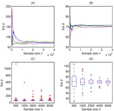
0 1 2 3 4 x 10⁵ 50 100 150 200 250 Sample size n Est d (A) 0 1 2 3 4 x 10⁵ 50 60 70 80 90 Sample size n Est d (B) 500 1000 2000 4000 8000 0 200 400 600 800 1000 (C) Est d Sample size n 500 1000 2000 4000 8000 40 50 60 70 80 90 100 (D) Est d Sample size n
Figure 1: Comparison of dbSM in UR (Uniform
Random) sampling and dbH in RW (Random
Walk) sampling. Panels A (for UR) and B( for RW) show that the estimation fluctuates with the increase of sample size. Panels C (for UR) and D (for RW) show the box plots of 100 es-timations for sample sizes ranging between 500 and 8000. The variance ofNbHH is var(NbHH) = 1 n N X i=1 pi(1/pi−N)2 (14)
It can be estimated from a sample using
d var(NbHH) = 1 n(n−1) n X i=1 (1/pi−N)2 (15)
Using Delta method the variance of estimatordH is
d var(dcH) =
s2
v
v4n (16)
wherevi = 1/di, v ands2v are the sample mean and
variance ofvi’s. This equation will be used in
calculat-ing the error bound in Figure 2.
3.
EXPERIMENTS
3.1
Data
The estimator is verified on the Twitter network data that are provided by Kwak et al. [12], characterizing the complete Twitter network as of July 2009. The data contain about 1.47 billion edges and 41.7 million
Table 1: Empirical bias and standard error of the two estimators over 100 runs for various sample size n.
Bias Standard error
n UR RW UR RW 500 2.6295 1.1444 108.1054 12.0539 1000 -4.1512 0.1016 53.8785 8.7383 2000 -0.8226 -0.0320 36.2923 5.6482 4000 4.0328 -0.2842 45.0989 4.1571 8000 2.1037 -0.0674 25.1908 2.7238
nodes or users, occupying around 20 gigabytes hard drive space. Since they are too large to fit into the memory of commodity computers, we index them using Lucene, a popular index engine. Then the random walk and uniform random sampling are performed on the in-dex that are stored in hard drive. Since our method is better to be used in undirected graph, we remove the direction in Twitter data.
3.2
Results
Two estimators,dbSM in Equation 1 anddbH in
Equa-tion 13, are tested on the data for five different sample sizes 500, 1000, 2000, 4000, and 8000. For each sam-ple size 100 samsam-ples are selected using uniform random sampling and random walk sampling respectively. Their bias and standard errors are tabulated in Table 1.
It shows that indeeddbH has a very small bias as
ex-pected. What is striking is that its standard error is much smaller than dbSM.
We use Figure 1 to explain the result further. Panels C is the box plot for dbSM using uniform sampling. It
shows that the estimation fluctuates very much, can even go as high as 1000 when n=500, where the true mean is 70.5. The big variance problem is ameliorated slightly but remains large with the growth of the sample size.
On the other hand the box plot for dbH in Panel D
shows much smaller variance.
We also run five large samples, each with size 4×
105, as depicted in panels A (for UR) and B (for RW). Note that in the case of uniform random sampling, the estimate jumps from time to time even when the sample size is rather large.
Figure 2 shows four estimations bounded by the 95% confidence interval calculated by Equation 16.
3.3
Discussions
This paper shows that the biased sampling is much better than uniform sampling for the estimation of av-erage degrees. In the past, people try to obtain uni-form samples whenever possible, and resort to biased
0 2000 4000 6000 8000 10000 40 50 60 70 80 90 100 110 120 sample size d Random walk
Figure 2: 95% confidence interval and four RW
(Random Walk) estimation processes using dbH
estimator. The error bound is drawn from Equa-tion 16.
sampling such as PPS (Proportional To Size) sampling only when uniform sampling is impossible [22] or costly. The results of this paper suggest that in the context of online social networks, random walk sampling instead of uniform sampling should be used, even when uniform random samples are readily accessible.
It is easy to understand that the variance of uniform random estimator dbSM is large because online social
networks are mostly scale-free as shown in Equation 9. The smaller variance ofdbH can be explained below.
LetdW be the random variable for the degrees
sam-pled by random walk. First we draw its empirical dis-tribution and its comparison with uniformly sampled degrees in Figure 3. Uniform random (UR) samples re-semble the distribution of the total population [23] that obeys power law with exponent around one. On the other hand, in random walk (RW) sampling schemedW
has a flatter starting section and a drooping tail, which can be approximated by the Mandelbrot law:
dWi = B
(a+i)b (17)
wherebis the exponent,B is a normalization constant,
ais a constant that corresponds to the position where the curve droops down.
Let v= 1 n n X i=1 1 dW i . (18) 100 102 104 106 100 101 102 103 104 105 106 107 rank degree RW UR
Figure 3: The degree distributions of the sam-ples obtained from UR (Uniform Random) and
RW (Random Walk) samplings. n=500,000.
The nodes, including the ones being repeatedly sampled, are ranked in decreasing order of their degrees, and drawn with degrees against their ranks.
The variance of the reciprocal of the variable is
var(1/dW) = n Pn i=1(i+a) 2b (Pn i=1(i+a)b) 2 −1 ! v2 = n n X i=1 (i+a)2b n X i=1 (i+a)b !−2 −1 v2 ≈ n 1 2b+ 1n 2b+1 1 b+ 1n b+1 −2 −1 ! v2 ≈ (b+ 1)2 2b+ 1 −1 v2
Thus var(1/dW) is a constant that does not grow
with the population size asσ2 does.
4.
IMPLICATIONS
Average degree plays a pivotal role in discovering other properties of a large network. Its accurate es-timation has a ramification on a string of other hidden properties of large networks. One immediate result is the total number of edges in the graph when user size is known. However, the more profound consequence is that we can discover the heterogeneity, CV (Coefficient of Variation), of the entire network with a small sam-ple using average degree. The discovery of CV will in turn deduce other properties such as the total number of users, the inequality of degrees (friends of friends and Gini coefficient).
4.1
Estimate heterogeneity
Vari-0 1000 2000 3000 4000 5000 6000 7000 800 1000 1200 1400 1600 1800 2000 2200 Sample size n Est CV sqr
Figure 4: 15 Estimation processes ofγ2in
Twit-ter data using Equation 20. The red dotted line is the true value.
ation (denoted as γ), that is an important metric to measure the heterogeneity of degree distribution. It is defined as the standard deviation normalized by the av-erage degree: γ2=σ2/d2. Expanding the definition for variance we have γ2+ 1 = d 2−d2 d2 + 1 = 1 N N X i=1 d2i " 1 N N X i=1 di #−2 =N N X i=1 d2i "N X i=1 di #−2
On the other hand the sample mean of the degrees ob-tained by random walk is
dW = 1 n n X i=1 dWi = N X i=1 pidi = 1 N d N X i=1 d2i (19)
Combining the two equations we derive the estimator for CV as follows:
b
γ2+ 1 = d
W
d , (20)
where dW is the sample mean of the degrees obtained
by random walk,dcan be estimated by the arithmetic mean of the same data. The convenience of the method is that only one random walk is needed. Figure 4 shows 15 estimates that converge quickly with the growth of the sample size.
4.2
Population estimation
Once γ2 is available, it can be used to estimate the population size as follows, which is a special case of Eq
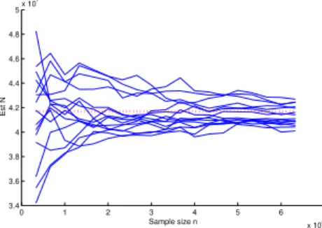
0 1 2 3 4 5 6 7 x 10⁴ 3.4 3.6 3.8 4 4.2 4.4 4.6 4.8 5x 10 7 Sample size n Est N
Figure 5: 15 estimation processes of twitter
ac-counts N using Equation 21. Red dotted line is
the true value.
3.20 in [2]: b N = (γ2+ 1) n 2 1 C, (21)
where n is the sample size, C is the number of colli-sions, and the sample is obtained by random walk2. In the area of capture-recapture research [2, 17, 15], it has been a perplexing problem for the population estima-tion of heterogeneous data whose capture probabilities are unequal, mainly due to the difficulty of estimating the heterogeneity. Now in the setting of OSN, the prob-lem is solved thanks to the estimator dbH.
Because of the accurate predication of the hetero-geneity of the data (γ2), the estimation of population size is rather good as shown in Figure 5. Since this es-timator hinges on collision times, extra caution should be taken to avoid spurious collisions caused by random walk. For instance if a node A is only connected to node B, a visit to A will cause node B visited twice. To avoid such loops, we take samples spaced every a few steps apart.
4.3
Other properties
4.3.1
Friends of friends
γ2can be also used to measure the ratio between the number of friends of your friends , and the number of your friends. As the saying goes, your friends have more friends than you do. To be more precise, your friends have γ2+ 1 times more friends than you do.
The mean number of friends of friends is [4]
N X i=1 d2i/ N X i=1 di=d+σ2/d (22)
2Here is a simple derivation for the estimator. The expected number of collisions is E(C) = n 2 ! N X i=1 p2i = n 2 ! 1 τ2 N X i=1 d2i = n 2 ! γ2+ 1 N
The above equation shows that your friends have no less than the friends you have. Simple rearranging the equation results in:
PN i=1d 2 i/ PN i=1di d = 1 +σ 2/d2 = 1 +γ2 (23)
In words, the equation says that on average your friends have 1 +γ2times more friends then you do. In a homo-geneous network where everybody has the same number of connections,γ= 0, thus your friends have the same number of friends as you do. In twitter society, γ2 is around 1000, thus your friends have a thousand times more friends than you do.
4.3.2
Message diffusion
Along the same lineγ2 can be used to quantify the diffusion of messages that is borrowed from epidemiol-ogy. In particular, it can be derived that the threshold for the occurrence of large component, or the occurrence of epidemics [9] (Eq 7.8) is
π=(γ
2+ 1)d−2
(γ2+ 1)d−1, (24) whereπis the proportion of the nodes that are immuned uniformly from the network.
4.3.3
Clustering Coefficient
Some structural network properties can be also de-rived using γ2. For instance, one important network property is Clustering Coefficient, indicating the pro-portion whether your friend of friend is also your friend. It is hard to calculate directly for a large network, but can be estimated [19] (eq 13.47) by
dγ4/n. (25)
4.3.4
Gini coefficient
Gini index is used to measure the inequality of wealth. It can also be used to measure the inequality of friend-ships in OSNs. Usingdthe Gini coefficient can be ap-proximated by b G= 1 2n(n−1)d n X i=1 n X j=1 |di−dj| (26)
The classic problem of Gini coefficient estimation is that the mean is hard to obtain. Thanks to the estima-tion of average degree, in Twitter network, we find its Gini coefficient is around 0.70-0.82.
5.
CONCLUSIONS
This paper proposes to use random walk to sample a network and use the harmonic mean to estimate the average degree. The empirical experiments show that
the estimator is much better even than uniform random samples.
The method is very practical in that in thousands or even hundreds of steps of random walk we can learn the average degree of a large network containing tens of millions of nodes and billions of edges.
The method works well because of the scale-free na-ture of the underlying network where the variance tends to be very large, potentially unlimited when the net-work size becomes infinitely large. For such netnet-works, we analytically showed that the harmonic mean estima-tor removed the large variance problem.
Therefore the estimator works not only for online social networks, but also any scale-free networks that are ubiquitous and more common than random net-works. For instance, we also validated the estimator in document-term graph where document and terms are nodes, and they are connected if a document contains a term.
The method relies on the assumption that random walk produces samples whose selection probability is proportional to their degrees. Theoretically this is true only asymptotically. Therefore the samples before the mixing time should be thrown away. Our experiments show little difference whether or not to include the first batch of samples in the random walk.
The degree estimation is not only important by itself but also crucial for discovering other network proper-ties. The success solution of average degree can lead to the discovery of the heterogeneity of the underlying data, the user and link size etc.
The method is not restricted to the degrees of the ex-plicit networks where the edges are the friendship rela-tions. Instead, the edges can be forged by other implicit relations, such as sharing the same message.
6.
ACKNOWLEDGEMENTS
We thank the reviewers for their detailed comments, and the support from NSERC (Natural Sciences and Engineering Research Council of Canada) and SSHRC (Social Sciences and Humanities Research Council of Canada).
7.
REFERENCES
[1] Z. Bar-Yossef and M. Gurevich. Random
sampling from a search engine’s index.Journal of
the ACM (JACM), 55(5):24, 2008.
[2] A. Chao, S. Lee, and S. Jeng. Estimating population size for capture-recapture data when capture probabilities vary by time and individual animal.Biometrics, pages 201–216, 1992.
[3] W. Cochran.Sampling techniques. Wiley-India, 2007.
[4] S. Feld. Why your friends have more friends than you do.American Journal of Sociology, pages
1464–1477, 1991.
[5] M. Gjoka, M. Kurant, C. Butts, and
A. Markopoulou. A walk in facebook: Uniform sampling of users in online social networks.Arxiv
preprint arXiv:0906.0060, 2009.
[6] M. Gjoka, M. Kurant, C. Butts, and
A. Markopoulou. Practical recommendations on crawling online social networks.Selected Areas in
Communications, IEEE Journal on,
29(9):1872–1892, 2011.
[7] M. Hansen and W. Hurwitz. On the theory of sampling from finite populations.The Annals of
Mathematical Statistics, 14(4):333–362, 1943.
[8] M. Henzinger, A. Heydon, M. Mitzenmacher, and M. Najork. On near-uniform url sampling.
Computer Networks, 33(1-6):295–308, 2000.
[9] M. Jackson. Social and economic networks. Princeton Univ Pr, 2008.
[10] L. Katzir, E. Liberty, and O. Somekh. Estimating sizes of social networks via biased sampling. In
Proceedings of the 20th international conference
on World wide web, pages 597–606. ACM, 2011.
[11] M. Kurant, A. Markopoulou, and P. Thiran. Towards unbiased bfs sampling.Selected Areas in
Communications, IEEE Journal on,
29(9):1799–1809, 2011.
[12] H. Kwak, C. Lee, H. Park, and S. Moon. What is twitter, a social network or a news media? In
Proceedings of the 19th international conference
on World wide web, pages 591–600. ACM, 2010.
[13] J. Leskovec and C. Faloutsos. Sampling from large graphs. InProceedings of the 12th ACM SIGKDD international conference on Knowledge discovery
and data mining, pages 631–636. ACM, 2006.
[14] L. Lov´asz. Random walks on graphs: A survey.
Combinatorics, Paul Erdos is Eighty, 2(1):1–46,
1993.
[15] J. Lu. Efficient estimation of the size of text deep web data source. InProceeding of the 17th ACM conference on Information and knowledge
management, pages 1485–1486, Napa Valley,
California, USA, 2008. ACM.
[16] J. Lu. Ranking bias in deep web size estimation using capture recapture method.Data &
Knowledge Engineering, 69(8):866–879, 2010.
[17] J. Lu and D. Li. Estimating deep web data source size by capture–recapture method.Information
retrieval, 13(1):70–95, 2010.
[18] N. Metropolis, A. Rosenbluth, M. Rosenbluth, A. Teller, and E. Teller. Equation of state calculations by fast computing machines.The
journal of chemical physics, 21:1087, 1953.
[19] M. Newman.Networks: an introduction. Oxford University Press, Inc., 2010.
[20] M. Papagelis, G. Das, and N. Koudas. Sampling
online social networks.Knowledge and Data
Engineering, IEEE Transactions on, (99):1–1,
2011.
[21] A. Rasti, M. Torkjazi, R. Rejaie, N. Duffield, W. Willinger, and D. Stutzbach.
Respondent-driven sampling for characterizing unstructured overlays. InINFOCOM 2009, IEEE, pages 2701–2705. IEEE, 2009.
[22] M. Salganik and D. Heckathorn. Sampling and estimation in hidden populations using
respondent-driven sampling.Sociological
methodology, 34(1):193–240, 2004.
[23] M. Stumpf, C. Wiuf, and R. May. Subnets of scale-free networks are not scale-free: sampling properties of networks.Proceedings of the National Academy of Sciences of the United
States of America, 102(12):4221, 2005.
[24] S. Thompson.Sampling. Wiley, 2012. [25] T. Wang, Y. Chen, Z. Zhang, T. Xu, L. Jin,
P. Hui, B. Deng, and X. Li. Understanding graph sampling algorithms for social network analysis.
Inthe 3rd ICDCS Workshop on Simplifying
Complex Networks for Practitioners, 2011.
[26] C. Wejnert and D. Heckathorn. Web-based network sampling.Sociological Methods &