Evaluation of the performance of deep learning techniques over tampered dataset

(1)

AL-HAMADANI, MOKHALED N. A., M.S. Evaluation of the Performance of Deep Learning Techniques Over Tampered Dataset. (2015)

Directed by Dr. Shan Suthaharan. 92 pp.

The reduction of classication error over supervised data sets is the main goal in Deep Learning (DL) approaches. However, tampered data is a serious problem in machine learning techniques. One of the recent interests to the machine learning community is the performance enhancement of supervised learning algorithms over tampered training data. In this thesis, the well-known deep learning techniques known as No-Drop, Dropout and DropConnect have been investigated by using toy example data set, the popular handwritten digits data set (MNIST), and our new natural images data set. The investigation divided into three groups which are training Deep Learning techniques over regular data sets, tampered data sets and noisy data sets. First, Deep Learning techniques have been investigated over regular data sets, the experiments showed good results in terms of accuracy and error rate. Then, Deep learning techniques were investigated with tampered MNIST data, this tampered mechanism is the rst step toward the security analysis of Deep Learning techniques. The results of DL techniques over tampered MNIST data set showed the same as in regular MNIST. Therefore, the investigation continued with adding two noises which were Gaussian noise and Salt and Pepper noise to reduce the clarity of the MNIST data set. The results showed that Deep Learning techniques still give good accuracy under noise eld environment. The thesis contribution is the extensive research that supports Deep Learning techniques that trained over tampered data to obtain high classication accuracy.

(2)

EVALUATION OF THE PERFORMANCE OF DEEP LEARNING TECHNIQUES OVER TAMPERED DATASET

by

Mokhaled N. A. Al-Hamadani

A Thesis Submitted to

the Faculty of the Graduate School at The University of North Carolina at Greensboro

in Partial Fulllment

of the Requirements for the Degree Master of Science

Greensboro 2015

Approved by

(3)

I would like to express my deepest gratitude to my family who are always supporting and encouraging me during my academic journey. To my beloved country "Iraq" despite all the unconditional situations over there, I have made it successful with your support. I will do my best to build you again. To my lovable

partner, you are always supporting and encouraging me in all the situations. I would like to thank all my Professors for their constant support through out the work, I wouldn't reach this point without your help and guidance. I would like to

(4)

APPROVAL PAGE

This thesis written by Mokhaled N. A. Al-Hamadani has been approved by the following committee of the Faculty of The Graduate School at The University of North Carolina at Greensboro.

Committee Chair

Shan Suthaharan Committee Members

Fereidoon Sadri Jing Deng

Date of Acceptance by Committee

(5)

ACKNOWLEDGMENTS

First of all, all the praise and thanks be to Allah for giving me the ability to complete my academic journey successfully.

I would like to thank the HCED (The Higher Committee For Education

Development in Iraq), who sponsored me to pursue my study in the United States of America.

I would like to express my deepest gratitude to my professor and advisor, Dr. Shan Suthaharan, for his excellent guidance, care, and patience during my thesis. I would not have been able to do the research and achieve learning in the same manner without his help and support.

(6)

IV. EVALUATION OF DEEP LEARNING APPROACHES . . . 41

4.1. Training Phase . . . 41

4.2. Testing Phase . . . 66

V. RESULTS AND FINDINGS . . . 84

5.1. Comparing DL Techniques with Regular Datasets . . . 84

5.2. Comparing DL Techniques with Tampered Dataset . . . 85

5.3. Comparing DL Techniques with Noisy Dataset . . . 86

VI. CONCLUSION AND FUTURE WORK . . . 88

(7)

LIST OF TABLES

Page

Table 1. Number of Observations in Training MNIST Dataset . . . 33

Table 2. Number of Observations in Testing MNIST Dataset . . . 34

Table 3. Number of Observations in Training New Puzzle Dataset . . . 38

Table 4. Number of Observations in Testing New Puzzle Dataset . . . 40

Table 5. Comparing Classication Error of DL Algorithms Using Regular Two-class Problems for the Three Datasets . . . 85

Table 6. Comparing Classication Error of DL Algorithms Using Tampered Two-class Problems for MNIST Dataset . . . 85

Table 7. Comparing Classication Error of DL Algorithms Using Noisy Two-class Problems for MNIST Dataset . . . 86

(8)

LIST OF FIGURES

Page

Figure 1. An Example of Neural Networks Layers . . . 9

Figure 2. An Example of Dropout Model . . . 12

Figure 3. An Example of DropConnect Model . . . 13

Figure 4. Our Model Layout for a Single DropConnect Layer . . . 14

Figure 5. Tanh Activation Function . . . 15

Figure 6. Sigmoid Activation Function . . . 16

Figure 7. Feed Forward Pass Steps . . . 19

Figure 8. An Example of No-Drop Model . . . 29

Figure 9. Histogram of Training MNIST Data Set . . . 32

Figure 10. Histogram of Testing MNIST Data Set . . . 33

Figure 13. Random Digits From MNIST Dataset . . . 35

Figure 14. An Example of New Puzzle Data Set . . . 37

Figure 15. Histogram of Training New Puzzle Data Set . . . 38

Figure 16. Histogram of Testing New Puzzle Data Set . . . 39

Figure 17. Evaluation of Deep Learning Approaches Architecture . . . 41

Figure 18. Error Rate of Training DropConnect Using Toy Example . . . 43

Figure 19. Training Results of DropConnect Model on Regular MNIST Dataset . . . 44

Figure 20. Before and After Attacking Digit 7 . . . 46

(9)

Figure 22. Before and After Attacking Digit 9 . . . 47

Figure 23. Training Results of DropConnect Model on Tampered MNIST Dataset . . . 47

Figure 24. The Visualizing of Regular and Noisy Digit 7 . . . 49

Figure 25. Training Results of DropConnect Model on Noisy Digit 7 . . . 50

Figure 30. Training Results of DropConnect Model on the New Puzzle Dataset . . . 54

Figure 31. Error Rate of Training Dropout Using Toy Example . . . 55

Figure 32. Training Results of DropOut Model on Regular MNIST Dataset . . . 56

Figure 33. Training Results of DropOut Model on Tampered MNIST Dataset . . . 57

Figure 34. Training Results of DropOut Model on Noisy MNIST Dataset . . . 59

Figure 35. Training Results of DropOut Model on the New Puzzle Dataset . . . . 60

Figure 36. Error Rate of Training No-Drop Algorithm over Toy Example . . . 61

Figure 37. Training Results of No-Drop Model on Regular MNIST Dataset . . . 62

Figure 38. Training Results of No-Drop Model on Tampered MNIST Dataset . . . 63

Figure 39. Training Results of No-Drop Model on Noisy MNIST Dataset . . . 65

Figure 40. Training Results of No-Drop Model on the New Puzzle Dataset . . . . 66

(10)

Figure 42. Testing Results of DropConnect Model on Regular MNIST

Dataset . . . 69

Figure 43. Testing Results of DropConnect Model on Tampered MNIST Dataset . . . 70

Figure 44. Testing Results of DropConnect Model on Noisy MNIST Dataset . . 71

Figure 45. Testing Results of DropConnect Model on New Puzzle Dataset . . . . 73

Figure 46. Error Rate of Testing Dropout Using Toy Example . . . 74

Figure 47. Testing Results of DropOut Model on Regular MNIST Dataset . . . . 75

Figure 48. Testing Results of DropOut on Tampered MNIST Dataset . . . 76

Figure 49. Testing Results of DropOut Model on Noisy MNIST Dataset . . . 77

Figure 50. Testing Results of Dropout Model on the New Puzzle Dataset . . . 78

Figure 51. Error Rate of Testing No-Drop Using Toy Example . . . 79

Figure 52. Testing Results of No-Drop Model on Regular MNIST Dataset . . . . 80

Figure 53. Testing Results of No-Drop Model on Tampered MNIST Dataset . . . 81

Figure 54. Testing Results of No-Drop Model on Noisy MNIST Datase . . . 82

(11)

CHAPTER I INTRODUCTION 1.1 Introduction

Recently, Deep Learning (DL) starts to play an essential role in data science [1]. Deep Learning has a layered-based architecture that has been motivated by articial intelligence [2]. These layers apply a nonlinear transformation that helps to extract the best features for classication problems. There have been dierent kinds of classication problems in DL methods which showed state-of-the-art results on dierent image recognition data sets in terms of the reduction of the error rate [3], [4], [5]. However, there's still a problem that has not been investigated yet in DL, which is the classication under dierent attack conditions. Recent studies showed that one of the machine learning techniques which is Support Vector Machine (SVM) has been aected by the attacking training data set [6]. They used a poisoning attacks over MNIST data set. In particular, they trained and tested two sub-class problems from MNIST data set. Their experiment results showed signicant increase in their classier's test error. For this reason, this thesis started to investigate the Deep Learning techniques which are known as DropConnect, Dropout, and No-Drop over tampered data set. Dropout is a form of regularization for fully connected neural network layers. It drops randomly some of the activations. DropConnect is a generalization of Dropout algorithm which is instead of dropping out some of the activations, it drops out some of the weights. In addition, No-Drop has the same concept of Dropout/DropConnect, but without dropping out any of the activations

(12)

or the weights. To evaluate DL techniques, There have been used three data sets. First, the popular handwritten (MNIST) data set which has 70,000 images ranging from 0 to 9. It is divided into two parts. The rst part has 60,000 training images and the second part has 10,000 testing images. Each digit is normalized and centered in a gray-level image with size 28 x 28 [7]. Moreover, for the purpose of this thesis, we have created two data sets. The toy example data set which has two classes 0 and 1 and each class has 50 samples. The third data set, called new puzzle natural images data set. It contains 26,197 natural images. It has been divided into two parts, training and testing. The training data set has 20,000 images and the testing data set has 6197 images. It has 7 classes from 0 to 6. The investigation started over regular two-class problems. The three data sets are used in this thesis have been divided into two-class problems. Deep Learning methods have been trained and tested over these regular data sets. The extensive experiments showed that Deep Learning methods can obtain lower error rate over regular data sets. The second part of the investigation was over tampered MNIST data set. In this thesis, we present our new attacking mechanism on two-class problem as the classication problem of SVM [6]. Our attacking mechanism is mixing two digits together from MNIST data set only and producing a new digit. After applying this attack, there is a tempered MNIST data set that may aect the performance of Deep Learning methods. These tampered two-class problems have been showed good results in terms of error rate. Moreover, the investigation continued with adding two dierent kinds of noise to MNIST data set only that can aect the images by adding some noise to their background. These noises are random variation of brightness or color information in the images [8]. We have chosen two dierent noises which are Gaussian noise and Salt and Pepper noise

(13)

for this problem. Gaussian noise is used to blur an image. Blurring the image can reduce the clarity or the resolution of the image, which may aect the performance of Machine Learning techniques. The second noise is the Salt-and-Pepper noise which is a one type of Impulse Noise which can corrupt the images, where the noisy pixels can take only the maximum and minimum values in the dynamic range [9]. In addition, it added randomly white or black pixels over the image. Salt-and-Pepper noise can have dark pixels in bright regions and bright pixels in dark regions. Therefore, we applied Deep Learning algorithms to the regular data sets, tempered MNIST data set, and noisy MNIST data set. The experiment showed that training under attacking data set still obtain lower error rate.

This thesis is structured as follows: Chapter II "Deep Learning (Structure and Methodology)" presents related work, neural networks, and Deep Learning and Deep Learning approaches; Chapter III "Data Set" presents several data sets that used in this research; Section IV "Evaluation of Deep Learning Approaches" presents the simulation of Deep Learning algorithms under dierent attack conditions with the machine learning phases; Chapter V "Results and Findings" presents the comparison of the classication error rate values for Deep learning approaches; and in Chapter VI the "Conclusion and Future Work" presents an overview for the whole research and points out some of the future work.

1.2 Machine Learning

Machine learning is a eld of study that works to build an algorithm that can learn from data [10]. Machine learning is a type of articial intelligence that provides computers with the ability to learn without being explicitly programmed [11].

(14)

Machine learning teaches the computer programs to learn with experience. For example, a spam lter classiers messages into spam or not spam. In other words, it tries to get the output that should be a yes or no indicting whether the message is spam or not. This example needs to have a set of input data with the corresponding output values. Machine learning algorithms train with taking the set of input, lets say x and repeatedly train with the input until it provides the output that can be closer to their corresponding outputs such as y. This is in training set. However, in testing set, the algorithms work to produce an output that can be either a spam message or not spam as in classication problems. Machine learning works with large data sets and try to classify them by using some algorithms. The more data is represented to machine learning method, the more classication can be accurate and gives better results. Machine learning tasks are grouped into two categories. The rst category is called supervised learning. The supervised learning is a type of learning that the training examples or data are labeled with the desired results. Supervised learning is like having a teacher telling you the right answer [12]. This learning is common in classication problems. For example, classication problems for pattern recognition, the algorithm train with the training set to compute outputs, then it compares the measured output with the desired output to compute the error rate of the classier. Classication problems are a type of supervised learning method that has a goal to minimize the error rate with respect to the given input. As much as the algorithm train with the set of inputs repeatedly, that much it learned and decreased the error rate. The second category called unsupervised learning. The unsupervised learning is much harder than supervised learning because the data set is unlabeled. This model is not provided with the correct results during the training. Unsupervised learning

(15)

is like learning without a teacher [12]. The goal of this type is to have the computer learn to do something without telling it how to do it. A type of unsupervised learning is called clustering. In this type of learning the goal is to cluster the input data in classes on the basis of their statistical properties [13]. This type of learning will not have names to assign to these clusters, it can produce a new example and then assign it to one of these classes based on the similarities of the data.

(16)

CHAPTER II

DEEP LEARNING (STRUCTURE AND METHODOLOGY) 2.1 Related Work

Recently many studies focus on classication of Deep Learning techniques over supervised and unsupervised data sets. The goal of all these studies is to get the better classication accuracy and less error rate. This research focuses on classication problems of deep learning techniques over supervised data sets. Following a list of some of the related

works:-Li, Zeiler, Zhang, Yann, and Rob have introduced a new algorithm in the Deep Learning eld called DropConnect which is a generalization of DropOut [3]. Their algorithm has a similar concept of the Dropout algorithm. However, DropConnect algorithm has a new technique which is randomly dropping out some of the weights instead of randomly dropping out some of the activations as it's in Dropout algorithm to avoid the over-tting problem. This technique shows signicantly better result in classication problems with fully-connected layers in Neural Network. They have used both of the algorithms in several datasets such as MNIST, CIFAR-10, SVHN, and NORB to check the accuracy and error rate. DropConnect algorithm showed state-of-art results on these datasets by getting less error rate among all the previous studies.

Hinton, Srivastava, Krizhevsky, Sutskever and Salakhutdinov have presented an algorithm called Dropout [4]. This algorithm applied to a fully-connected layers within neural networks. Dropout algorithm is randomly dropping out some of the

(17)

activations. This technique improves network generalization ability and improves the test performance. It also reduces the overtting problems. They have tested Dropout algorithm in batch of data sets including (speech and object recognition) which showed new record comparing to other algorithms.

Dan, Ueli, and Jurgen have presented a new method which is combing several Deep Neural Networks (DNN) columns into a multi-column Deep Neural Networks (MCDNN) [14]. This new technique has matched the human performance on some tasks such as recognition of handwritten digits and trac signs. In this technique, they took only the winner neurons to train them. They used several data sets to test their method such as MNIST, Latin letters, Chinese characters, trac signs, NORB, and CIFAR-10. They used graphic cards (GPU) to make the training much faster. This method shows state-of-art on MNIST data set and several other image data sets that were close to human performance.

Xavier Frazao and Luis Alexandre have introduced a new algorithm which is called DropAll [15]. This method is a generalization of combing the two well-known methods for regularization of convolutional neural networks which are Dropout and DropConnect. Dropout and DropConnect algorithms were dropping out randomly from the activations or the weights, respectively. In this algorithm, they used to DropAll from the activations and the weights together to avoid over-tting with using a new method of combing networks. They used a common data set which called CIFAR-10, which is a natural images data set. Their results in this data set showed the improvements of their technique in terms of the accuracy and the error rate than Dropout and DropConnect.

(18)

2.2 Neural Networks 2.2.1. Historical Background

Neural Networks begin in the early 1940's by McCulloch and Pitts [16], when they introduced the rst neural network computing. Several years later, and specically in 1985, Rosenblatt developed and designed the perceptron [17]. The perceptron has three layers, the rst layer for input units, the middle layer as an association layer, and the nal layer as an output layer. Perceptron design was capable to recognize simple numerics. However, this design was not capable to solve problems like the XOR problem. Then, in 1974, Paul Werbos developed the Back-propagation learning method which is one of the most important methods nowadays in neural networks [18]. Therefore, the progress of developing neural networks during 1970's to early 1980's were important to elevating the neural networks eld. Finally, researchers have kept working on developing neural networks with dierent applications such as pattern recognition and several other applications.

2.2.2. Neural Networks

Neural Network is an information processing method that has been inspired by the biological nervous systems, in particular the brain [19]. Neural Networks work to solve problems that are too complex. These problems can be solved by a human being easily, but it's too complicated for a computer to do it, such as pattern recognition. Neural networks learn from the experience instead of being explicitly programmed [20]. Neural network is also known as an articial neural network or neural sets. Neural Network consists of three groups of layers. The rst group is called the input layer which is connected to a layer of hidden units. The second group called the hidden layer, which is connected to a layer of output units and is the last group of

(19)

layers, as shown in gure 1. Moreover, neural networks architectures can be grouped into two categories [21].

Figure 1. An Example of Neural Networks Layers

First category is called Feed-forward networks which is a simple neural network method is a set of connections from the input layer to the hidden layer and then to the output layer, which means that neural networks are organized in hierarchical architecture. This method works to produce one output from the data set or set of outputs of the networks by moving the data from the input layers to the hidden layer by non-linear transformation activation function after passed on and weighted. These outputs would be the inputs for the next hidden layers and so on until it provides the outputs by the output layer. These outputs can be compared with the actual outputs of the data set in terms of supervised learning. This step measures the error rate of the feed forward method. The second category called Back-propagation algorithm. This algorithm works to reverse the steps of feed forward method. In this algorithm

(20)

the network can measure the derivative of the error of feed forward with respect to the weight parameters. It works to minimize the error rate of the network until it gets closer to producing the desired output. These two categories are described in detail in Deep Learning Approaches section.

2.3 Deep Learning (DL)

Deep Learning is a recently developed eld which is a new area in machine learning methods, although it belongs to Articial Intelligence. Deep Learning emulate to imitate the human brain by analyzing, learning, and solving dierent kinds of complex problems. It's derived from the concept of Articial Neural Networks (ANN) and utilize learning algorithms that are inspired by our understanding of how the brain learns. However, Articial Neural Networks algorithms are assessed basing on how well they work for practical applications such as speech recognition, object recognition, and handwritten digits. In addition, Deep Learning algorithms have a layered-based architecture. These layers apply nonlinear transformation functions to its input neurons and it provides outputs [22]. These outputs would be the input for the next layers and passed on and weighted and transformed by some functions to the next layers. Finally, the output layers give the output that determine which input has been read. These steps are known as a Feed Forward phase. As we mentioned that DL has the concept of ANN, then it has the architecture of Feed Forward and Back-Propagation. In the Back-Propagation phase, the network works to update the weight parameters by inverting the steps of Feed Forward. For this reason, it's also known as Feed Backward.

(21)

2.4 Deep Learning Approaches

Deep Learning has recently proposed two approaches which are DropOut and DropConnect for regularizing large fully connected layers in neural networks [3], [4]. These two approaches reduce the over-tting problems and improve the test performance. These algorithms have been trained and tested by several data sets and give the state-of-art results. The following sections describe these two approaches. 2.4.1. Dropout

Dropout was presented by Hinton in 2012. This algorithm was a form of regularization for fully connected neural network layers [4]. Dropout is applied to the output layer's where each element is kept with probability p, otherwise being set to 0 with probability (1−p). If the Dropout algorithm is applied to the outputs of a fully connected layer, then the equation can be written

as:-r =m∗a(W v)

where m is a binary mask vector of size dwith each element j coming independently from a Bernoulli distributionmj Bernoulli(p) when p = (0.5), W is a weight matrix

with fully connected layers, v is the input vector, andais an activation function, such as in our case ( tanh and Sigmoid). Figure 2 shows the Dropout model.

(22)

Figure 2. An Example of Dropout Model

This algorithm showed better results with several data sets by dropping out half of the activations randomly in each iteration. This was the key of reducing the over-tting problems with training large data sets within neural networks.

The training Dropout model can be described as the

following:-(1) Selecting an example v from the training data set and multiplying it with the weight matrix, then apply an activation function (tanh and Sigmoid) to it. Therefore, mask out element by element the product.

(2) The results in r would be the input of the soft-max function which predicts the class probability of the classication problem.

(3) The prediction output results are used to compute the error rate of the classication problem by comparing them with the true output by using cross-entropy function.

All these steps are known as a forwards pass. For Backwards or back-propagation has used a standard mini-batch Stochastic Gradient Decent algorithm to update the weight parameters. Mini-batch SGD works by taking the derivative of cross-entropy

(23)

function with respect to weight parameters. Feed forwards and back-propagation are described in more detail in DropConnect's section.

2.4.2. DropConnect

DropConnect is a recent algorithm in Deep Learning eld, and it's a generalization of Dropout algorithm. DropConnect algorithm is similar to the concept of Dropout algorithm, but it diers in one thing, which is instead of dropping out some of the activations as in Dropout, it drops some of the weights in DropConnect. For DropConnect algorithm, the output can be written

as:-r=a((M∗W)v)

where M is a mask matrix for the weight parameter and mij Bernoulli(p) when p

= (0.5) also as in Dropout algorithm, W is a weight matrix, v is an input vector, and a is an activation function for either (tanh or sigmoid). This technique showed better results than the previous techniques of the Deep Learning method which are (Dropout and No-Drop) [3]. Figure 3 shows the Dropconnect model.

(24)

This model has the same architecture as the Dropout model. In [3] four basic components for DropConnect model have been mentioned, which are feature extractor, DropConnect layer, softmax classication layer, and cross entropy loss. In this research work, the rst component which is the feature extractor, it has been skipped and it has been assumed that the features are extracted already.

Figure 4. Our Model Layout for a Single DropConnect Layer

Therefore, the DropConnect model has three fundamental components as shown in gure 4 that have been inspired from original model in [3]. The description of DropConnect model is as

follows:-(1) Input

Features:-V=(n x 1), where v is the input vector of the DropConnect model. V is one image features or pixels from the benchmarks data sets that are used in this research.

(2) Activation

Function:-There are lots of activation functions that have been used within Neural networks. These activation functions are non-linear functions and used to transform the activation level of neurons that have been weighted and summed

(25)

to an output layer. The output of the activation function can be either 0 or 1 and it depends on the input. In this research, we have used the two most common activation functions, which are (tanh and sigmoid).

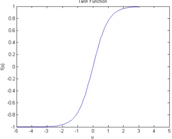
• tanh (Hyperbolic Tangent

Function):-Tanh is the hyperbolic tangent function. Function):-Tanh is derived from the hyperbolic sine and the hyperbolic cosine functions, then it can be written

as:-tanh(u) = sinh(u) cash(u)

Hyperbolic Tangent Function is a scaled and shifted version of Sigmoid function and its output range is from (1-, 1) [23] as shown in gure 5. Tanh usually converges faster than Sigmoid function [24].

(26)

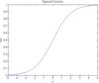
• Sigmoid (Standard Logistic

Function):-Sigmoid is the standard logistic function. The Function):-Sigmoid function is also called the sigmoidal curve [25], this function can be written

as:-Sigmoid= 1 1 + exp(−u)

The logistic function(Sigmoid) output is in the range of (0,1) as shown in gure 6. This function is similar to the input/output of biological neurons [26]. Another key point is that the derivative of the Sigmoid activation function is easy to calculate.

r=a((M ∗W)v)

Therefore, activation functions that are used in the above equation have also a weight parameter and Mask matrix.

(27)

• Weight Parameter

W:-Weight parameter is one of the main components in the DropConnect model because it helps the model to determine which digit has been read. It's a fully connected weight matrix that has been generated randomly for the rst iteration in the range of (0,1). Then these weight parameters can be updated by using Stochastic Gradient Descent.

• Mask

M:-Mask is a binary matrix and mij Bernoulli(p) when p = (0.5). It

generates randomly during the training and testing phase. It's the main key component for training successfully with the DropConnect model because it generates randomly for each single training example. This matrix helps the DropConnect algorithm to drop or re some of the weights or neurons as it called in Neural Network. The purpose of this operation is to keep some of the weight values that can help the algorithm to determine which digits have been read during training and testing phases.

(3) Softmax

Function:-Softmax activation function is a neural transfer function [27]. Function:-Softmax function is a supervised learning algorithm. It calculates the neural output from its input vector. It gives the probabilities of k values in the range of (0,1). Softmax function make sure that the summation of the probability has to be 1. Soft-max function allows to use the cross-entropy loss function to compute the error rate of the classication problem [28]. Softmax function can be written

(28)

as:-o= _P_nexp(W sj ∗r)

k=1exp(W sk∗r)

wherekis the number of classes it uses output of the activation function r as an input, and with the new weight parameter Ws, this weight parameter generates randomly for the rst iteration same as W, and it can be updated by SGD. This equation leads to predict the probability for the class that has been read. (4) Cross Entropy

Loss:-Cross Entropy or Error Function is a function that measures the error that compares computed output values with the known target desired output values of some training data. Cross entropy can be written as

A(i) =−

K

X

i=1

yilog(oi)

where K is the number of classes for any data set, yi are the labels of training

data of any data set or the ground truth labels [3], and oi is the target desired

output values of training data or the probabilities that are computed by Soft-max function.

The above points were the description of the Dropconnect model. They are also the Feed Forward pass step of the DropConnect algorithm as shown in gure 7. Training with DropConnect requires Feed Forwards and Back-propagate gradient. These two techniques are described as

(29)

follows:-Figure 7. Feed Forward Pass Steps

Figure 6 summarizes the Forward pass steps. Forward pass is computing activations and Soft-max output by selecting an example v which assumed that the features are extracted. These features are the input for activation function where a mask is rst drawn from a Bernoulli(p) when p = (0.5) distribution to mask out elements of weight matrix (W) that has been generated randomly. As mentioned above, the mask generates randomly in each iteration and this is the key of successfully training with DropConnect. Then, the masked weight is multiplyed with the input v. Therefore, the output of this multiplication

(30)

(u) can be the input of the activation functions. The result of the activation function (r), is the input of the Soft-max activation function with the new weight parameter which is (Ws) which predict for us the probability of the digit that has been read. Finally, it computes the cross-entropy (error rate) by multiplying the soft-max function output, which is (o), the predicted value of the current digit with the truth values of the digit to see the error rate of detecting the corresponding digit.

(5) Backpropagate

Gradients:-In this step, the DropConnect model use Stochastic Gradient Descent to compute the derivative of the entropy with respect to the weight parameters. However, there are three dierent gradient methods, which are gradient descent, stochastic gradient descent, and mini-batch stochastic gradient descent. All these methods are important optimization techniques, which are trying to minimize the error function by taking the derivative of the cross-entropy function with respect to weight parameters. Therefore, this research explains the three techniques with their advantages and disadvantages as

follows:-• Gradient Descent

(GD):-Gradient Descent is an algorithm that minimizes error functions. It takes m examples in each iteration, where m is the whole data-set observations. Then it calculates all the derivative (di) where i=1 to m. Then it sums the derivative for all (di) and updates W and Ws as

follows:-W =W0−α

X di

(31)

where W0 is the initial weight that generated randomly, α is the

learning rate, P

di is the summation of all the derivatives, and W is the

new updated weight parameter. However, this method is really slow because it takes m examples, where m is the whole data-set, and it computes the derivative for all of them to update a single weight parameter [24]. Also, it can be intractable on a single machine if the data-set is too big to t a main memory.

• Stochastic Gradient Descent

(SGD):-Stochastic Gradient Descent (SGD) or online learning is a gradient descent optimization method for minimizing the entropy function by taking the derivative of the cross-entropy function with respect to weight parameters [24]. In other words, it's an understanding of how changing weights in a network would change the cross-entropy function. SGD works to update the weight parameters (W and Ws) in Deep Learning techniques. This is an optimization method of GD as mentioned above, and it also works much faster than GD because SGD takes one example in each iteration [29]. It calculates the derivativedj at each step or for each single example.

Then, it updates the currentW with the localdi as follows:-Wi =Wi−1−αdj

where Wi − 1 is the initial weight for the current example, Wi is the

updating weight parameter for the current example or for each example that we want to update in SGD, α is the learning rate, and dj is the

(32)

• Mini-Batch Stochastic Gradient Descent (Mini-Batch

SGD):-Mini-Batch Stochastic Gradient Descent has the same concept as SGD and GD; therefore, it mixes both of the techniques to come up with mini-batch SGD. It works faster than GD and it takes samples of data n from the whole data set in each iteration [24]. Then it calculates all the derivatives (di) where i=1 to n. Then it sums the derivative for all (di) and updates W and Ws as

follows:-W =W0−α

X di

where W0 is the initial weight that generated randomly, α is the

learning rate, P

di is the summation of all the derivatives, and W is the

new updated weight parameter.

In this research, stochastic gradient descent (SGD) has been used to update the weight parameters.

The learning rate α has been seen in both Stochastic Gradient Descent and Gradient Descent. The learning rate is used to minimize the updated weight parameters. The learning rate is dierent from GD to SGD and it is much smaller in SGD than the corresponding learning rate in Batch Gradient Descent because there is much more variance in the update [29]. Therefore, SGD should use a small enough constant learning rate that can give stable convergence in the learning set. One more point about the learning rate is that it can be changed manually if the network stops improving as mentioned in [3].

Now, the derivative can be given by calculating one example to update the weight parameters. So, there are two derivatives in this thesis for Backpropagate

(33)

gradient, which are ∂E

∂W ( this is the derivative of entropy with respect to weight

parameter (W)) and ∂E

∂Ws (this is the derivative of entropy with respect to soft-max function's weight parameter (Ws)).

• ∂E

∂W is the derivative of entropy with respect to weight parameter W.

This derivative can be divided into three derivatives to simplify it as the following:-∂E ∂W = ∂E ∂oj ∗ ∂oj ∂r ∗ ∂r ∂W where ∂E

∂oj is the derivative of the entropy E with respect to the Soft-max function(o), ∂oj

∂r is the derivative of the Soft-max function (o) with respect

to activation function(r), and _∂W∂r is the derivative of the activation function (r) with respect to weight parameter (W).

This has been done to simplify the SGD and make it much easier to understand. Here is the mathematical derivative for the above.

• ∂E

∂oj is the derivative of the entropy (E) with respect to the Soft-max function (o) which is the

following:-∂E ∂oj =−Xyy∗log(oj) = −yy∗ 1 oj (2.1)

where yy is the truth table of the true labels of the data sets and log(oj)

is the probability of the digit that is being computed during the forward pass step.

(34)

• ∂oj

∂r is the derivative of the soft-max function (o) with respect to activation

function (r). ∂oj ∂r = exp(W sj∗r) Pn k=1exp(W sk∗r)

where the W sj is the weight parameter for only one example that we are

training and dividing it by the summation of all the examples which isW sk,

and the above equation is the soft-max function whereo= exp(W sj∗r)

Pn k=1exp(W sk∗r). ∂oj ∂r = exp(W sj∗r) Pn k=1exp(W sk∗r) = [ Pn k=1exp(W sk∗r)∗W sj ∗exp(W sj∗r)] [Pn k=1exp(W sk∗r)]2 −[exp(W sj ∗r)∗ Pn k=1W sk∗exp(W sk∗r)] [Pn k=1exp(W sk∗r)]2 = W sPnj ∗exp(W sj∗r) k=1exp(W sk∗r) − exp(W sj ∗r)∗ Pn k=1W sk∗exp(W sk∗r) [Pn k=1exp(W sk∗r)]2 =W sj ∗oj − exp(W sj ∗r) Pn k=1exp(W sk∗r) ∗ Pn k=1W sk∗exp(W sk∗r) [Pn k=1exp(W sk∗r)]2 =W sj ∗oj−oj∗ Pn k=1W sk∗exp(W sk∗r) [Pn k=1exp(W sk∗r)]2

(35)

=oj W sj − Pn k=1W sk∗exp(W sk∗r) [Pn k=1exp(W sk∗r)]2 (2.2)

Then, from (2.1) and (2.2) we get the following (2.3).

∂E ∂oj ∗ ∂oj ∂r =−yy∗ 1 oj ∗oj W sj − Pn k=1W sk∗exp(W sk∗r) [Pn k=1exp(W sk∗r)]2 =−yy∗W sj −(−yy)∗ Pn k=1W sk∗exp(W sk∗r) [Pn k=1exp(W sk∗r)]2 (2.3) • ∂r

∂W is the derivative of the activation function (r) with respect to the weight

parameter (W).

∂r ∂W =

1 1 + exp(−u)

where the equation above is the activation function r = _1+exp(1 ₋_u) and u is the multiplication of Weight parameter W with Mask M and the input examplev. ∂r ∂W = 1 1 + exp(−u) = 1

1 + exp(−u)∗(exp(−u)) = 1 1 + exp(−u)∗ 1− 1 1 + exp(−u)

(36)

=r∗(1−r) (2.4) Then the derivative of EntropyE with respect to weight parameter W is

∂E ∂W =Equation (2.3)∗Equation(2.4). ∂E ∂W = ∂E ∂r ∗ ∂r ∂W. (2.5) • ∂E

∂W s is the derivative of the Entropy with respect to the weight parameter

W s.

This derivative is divided into two parts as well as ∂E

∂W. Here is the

simpli-cation of this part.

∂E ∂W s = ∂E ∂oj ∗ ∂oj ∂W s • ∂E

∂oj is the derivative of the EntropyE with respect to the soft-max function oj which is the same as equation (2.1).

• ∂oj

∂W s is the derivative of the Soft-max functionoj with respect to the weight

parameterW s. ∂oj ∂W s = exp(W sj∗r) Pn k=1exp(W sk∗r)

where the W sj is the weight parameter for only one example that we are

training and dividing it by the summation of all the examples which isW sk,

and the above equation is the soft-max function whereo= exp(W sj∗r)

Pn

(37)

∂oj ∂r = exp(W sj∗r) Pn k=1exp(W sk∗r) = [ Pn k=1exp(W sk∗r)∗r∗exp(W sj ∗r)] [Pn k=1exp(W sk∗r)]2 −[exp(W sj∗r)∗ Pn k=1r∗exp(W sk∗r)] [Pn k=1exp(W sk∗r)]2 = Prn∗exp(W sj ∗r) k=1exp(W sk∗r) −exp(W sj ∗r)∗ Pn k=1r∗exp(W sk∗r) [Pn k=1exp(W sk∗r)]2 =r∗oj − exp(W sj ∗r) Pn k=1exp(W sk∗r) ∗ Pn k=1r∗exp(W sj ∗r) [Pn k=1exp(W sk∗r)]2 =r∗oj −oj ∗r∗ Pn k=1exp(W sj ∗r) [Pn k=1exp(W sk∗r)]2 =R∗oj−oj∗oj∗r =oj(1−oj)∗r (2.6)

In some points we don't need W sk because if we have k = 10, then we

will need only W sj between all the k. Therefore, it take asW sj from this

point.

Then the derivative of Entropy E with respect to weight parameter W s is ∂E

(38)

∂E ∂W s = ∂E ∂oj ∗ ∂oj ∂W s =−yy∗ 1 oj ∗oj(1−oj)∗r =−yy∗(1−oj)∗r (2.7) 2.4.3. No-Drop

No-Drop is the third technique that has been used in this research. This method has the same concept as Dropout and DropConnect, but without dropping out any activations or weights. The No-Drop algorithm is applied to the outputs of a fully connected layer, then the equation can be written

as:-r =a(W v)

where W is a wight matrix with fully connected layers, v is the input vector, and a is an activation function such as in this thesis ( tanh and Sigmoid). Figure 8 shows the No-Drop model. Training with No-Drop is the same as in both previous techniques (Dropout and DropConnect). This model showed some good results by training and testing it with some data sets as mentioned in [3]. However, Dropout and DropConnect models are better than this technique as mentioned in [3].

(39)

Figure 8. An Example of No-Drop Model

The Dropout and DropConnect methods work together to prevent the over-tting by using mask vector/matrix. This technique doesn't use mask.

(40)

CHAPTER III DATA SET 3.1 Toy Example Dataset

We created a two-dimensional toy example data set. It has two classes assigned as (0 and 1). For class 0, we generate random positive numbers in the range of (10, 20). For class 1, we generate random negative numbers in the range of (-10, -20). The training and testing sets consist of 50 and 20 points per class, respectively. This toy example is a perfect way to validate the models of Deep Learning.

3.2 MNIST Dataset

MNIST is the most popular handwritten digits data set which contains thousands of scanned images of handwritten digits with their actual labels. MNIST data set comes from the subset of two data sets that are collected by NIST (National Institute of Standards and Technology) [22]. A MNIST data set contains 70,000 images of handwritten digits (0 through 9). These digits have been divided into two parts. The rst part contains 60,000 images for training sets. These images are scanned handwritten samples from 250 people. Those 250 people were divided into two halves where the rst half were employees in the US Census Bureau and the second half were high school students. These images have been normalized by using some normalizing algorithm and centered in (28 x 28) = 784, gray scale pixels [7]. These pixels are a dimensional vector represents the features in the MNIST data set. Moreover, each pixel in the MNIST data set is represented by a value between 0 and 255, where 0 is

(41)

black and 255 is white and anything in between is represented by a dierent shade of gray.

The training part in the MNIST data set itself is divided into two parts. The rst part contains 50,000 images as a training set and 10,000 images as a validation set. The second part of the MNIST data set contains 10,000 images as a testing set. However, these 10,000 images were taken from 250 dierent people (People were from the same two organizations, USCB employees and high school students) in order to make it a good test of performance. In addition, this can help us to evaluate the performance of DL algorithms who have been trained by images weren't written by the same people.

3.2.1. Analyzing MNIST Data Set

MNIST data set is a large data that can be hard to understand without simplifying or analyzing it. Therefore, MNIST has two parts as we mentioned before which are training and testing data set and both contains 70,000 images. To analyze this, we have to know the number of digits in each part and the ratio of them in order to observe if it is a balanced data set or unbalanced data set.

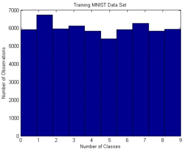
(1) Training Data set

This part has 60,000 images of handwritten digits (0 to 9). The ratio of the training set is shown in the gure 9.

(42)

Figure 9. Histogram of Training MNIST Data Set

From gure 9 we observed that the training part of MNIST data set is balanced because they almost have close to 6000 observations or images for each digit. However, for curiosity we analyzed it more to see how many observations or images each digit has. Table 1 shows the number of observations with the corresponding digits.

(43)

Table 1. Number of Observations in Training MNIST Dataset Training MNIST Dataset Digit Numbers Number of Observations

0 5932 1 6742 2 5958 3 6131 4 5842 5 5421 6 5918 7 6265 8 5851 9 5949

(2) Testing Data Set

This part has 10,000 images of handwritten digits (0 through 9). The ratio of the testing set of MNIST data set is shown in gure 10.

(44)

The same as in the training data set, we observed from gure 10 that the testing part is balanced too because each digit has almost close to 1000 images or observations. Table 2 shows the specic number of observations with the corresponding digits in the testing data set.

Table 2. Number of Observations in Testing MNIST Dataset Testing MNIST Dataset Digit Numbers Number of Observations

0 980 1 1135 2 1032 3 1010 4 982 5 892 6 958 7 1028 8 974 9 1009

For further analysis, it's quite hard to determine which feature is good for the classication problem. However, we started to analyze more by plotting a histogram of dierent images from the training data set along with the visualizing of the corresponding images. That can show the best features for the classication problem. We took random images as an examples as shown in the below gures.

(45)

(a) Digit (1) (b) Histogram of Digit(1)

Figure 13. Random Digits From MNIST Dataset

From them above gures, we determined that we have lot of 0's which are the dark regions in the images which can't help our algorithms in the classication problem. These regions can be cropped in order to use the only light region or that has the

(46)

digit. However, it's handwritten digits which have been written in dierent ways, so it might have digits written in the center, left or the right side of the image based on the digits as shown in the gure 13. These gures shown how the digits have dierent locations. Therefore, in order to crop an image, it has to be done randomly. So, that can give the high probability of getting the whole digit in the images.

3.3 New Dataset

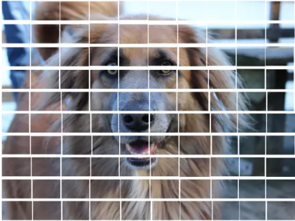
For the purpose of this thesis, it has been created a new natural images data set. These images have been taken by using a professional camera Canon T3i. This data set contains images of bears, dogs, cars, cats, ducks, beaches, and sunsets. Each category contains between 35 to 39 images. However, training and testing data must be larger in order to train any model perfectly. Therefore, we came with a new idea which was dividing each image into 100 pieces and turning it into puzzle data set. Figure 14 shows an example of the dog puzzle picture. Puzzle are a well known activity and they need time to collect all of the pieces to make a picture as a human being. For this reason, this new idea came to check the performance of Deep Learning methods with this new puzzle data.

(47)

Figure 14. An Example of New Puzzle Data Set

The puzzle data set consists of 26197 images in 7 classes. These images are scaled down and re-sized to 28 x 28 pixels as in MNIST data set [7]. Also, these images were converted from color images into gray images. Each class contains between 3500 to 3900 images. We labeled them as MNIST data set, when class bear has class label as 0 to class sunset has class label as 6. This data set has been divided into two parts. The rst part contains 22,000 images for training set and the second part contains 4197 images for testing set.

3.3.1. Analyzing New Data Set (1) Training Data set

This part of the Puzzle data set contains 22,000 natural images within 7 classes from (0 through 6). The ratio of the training set is shown in gure 15. Figure 15 shows that the training new puzzle data set classes are very close to each

(48)

other which is a balanced data set. Also, in table 3, it has been provided the number of observations of each class with the corresponding digits or categories.

Figure 15. Histogram of Training New Puzzle Data Set Table 3. Number of Observations in Training New Puzzle Dataset Training New Puzzle Dataset Digit Numbers Number of Observations

0 2990 1 3196 2 3218 3 2934 4 3023 5 3386 6 3253

(49)

(2) Testing Data Set

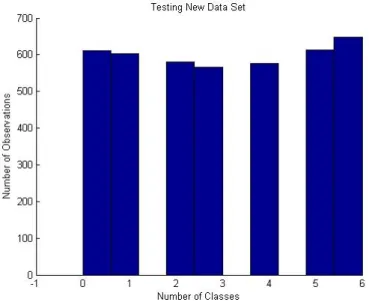
This part of Puzzle data set contains 4197 natural images within 7 classes from (0 through 6). The ratio of training set is shown in gure 16.

Figure 16. Histogram of Testing New Puzzle Data Set

Figure 16 shows that the training new puzzle data set classes are very close to each other which is a balanced data set. Therefore, there's no need to make the data balance by adding more samples or duplicating the number of sample in each category. For further analyzing, we have provided a table that contains the exact number of sample for each category, that can give a clear picture of how close are the number of samples and proved that the data set is balanced.

(50)

Table 4, it provided the number of observations/samples of each class with the corresponding digits or categories.

Table 4. Number of Observations in Testing New Puzzle Dataset Testing New Puzzle Dataset Digit Numbers Number of Observations

0 610 1 603 2 581 3 566 4 577 5 613 6 647

(51)

CHAPTER IV

EVALUATION OF DEEP LEARNING APPROACHES

The evaluation of Deep Learning approaches has been divided into two parts, training and testing. The three data sets have been divided into 80 percent for training and 20 percent for testing. The three approaches of DL which are, DropConnect, Dropout, and No-Drop have been trained and tested using toy example data set, MNIST data set, and new puzzle data set. The chapter description is shown in gure 17.

Figure 17. Evaluation of Deep Learning Approaches Architecture

4.1 Training Phase

The training phase is used to train the model and choose the optimum parameters for a given model, by comparing the input with expected output. Training

(52)

phase section has been divided into three parts, training with DropConnect, Dropout, and with No-Drop. The attacking mechanism and noise environment have been added to MNIST data set only. The other data sets trained and tested in the regular way without having any attacking or noisy conditions. The investigations for the three approaches have been done similarly to [30], we investigated on two-class sub-problems. In particular, for MNIST data set has been taken the following two-class problems: 1 and 7; 1 and 8; 1 and 9. Then, it has been added attacking and noisy conditions to these two-class problems. Therefore, MNIST data set has three cases which

are:-(1) Regular Two-class Problems (2) Tampered Two-class Problems (3) Noisy Two-class Problems

• Gaussian Noisy Two-class Problems

• Salt and Popper Noisy Two-class Problems

For toy example data set and new puzzle data set have been taken only the regular two class problems. In particular, for new puzzle data set that has been taken the following two class-problems, dogs and bears, dogs and cats, and dogs and ducks. 4.1.1. Training with DropConnect

The training of DropConnect algorithm for single layer neural networks has been done using toy example data set, MNIST data set, and new puzzle data set. The training of Dropconnect algorithm has been used a Stochastic Gradient Descent for all the experiments with the learning rate equal to (0.0001). The evaluation of the DropConnect algorithm has been done as the following

(53)

(1) Training DropConnect Model Using Toy Example Data Set

The toy example data set has two classes which are, class (0) and class (1), which each class has 50 samples. The data set has been shued before training DropConnect algorithm with it. Figure 18 shows the error rate of the training DropConnect using toy example.

Figure 18. Error Rate of Training DropConnect Using Toy Example

The error rate of training DropConnect over toy example was 0.2370. That means if there are more samples in the toy example, it may reduce the error rate to lower than 0.2370.

(2) Training DropConnect Model Using MNIST Data Set

The training MNIST data set contains 60,000 images from 0 to 9 (10-classes). Each digit in the training set is normalized to t 28 x 28 pixels. These pixels have values between 0 and 255, it has been scaled the pixel values into [0,1] range before training DropConnect model. As mentioned before, the MNIST data

(54)

set has been divided into three parts. Therefore, the training of DropConnect algorithm using MNIST data set has been done as the following

:-• Regular MNIST Two-class Problems

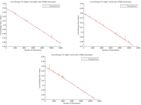
The DropConnect algorithm has been trained using regular MNIST two-class problems. First two two-class problems were (1 and 7) which have 6000 and 6000 sample, respectively. The second and third two-class problems were (1 and 8) and (1 and 9) which have 6000 and 5000 samples, respectively. Figure 19 shows the error rate of the training phase of those three cases.

Figure 19. Training Results of DropConnect Model on Regular MNIST Dataset

Figure 19 clearly shows the results of training DropConnect model on multi-run experiments with these three regular cases which shows that

(55)

the model trained well. It gave a lower error rate for (1 and 7) two-class problems which was equal to (0.4575). Moreover, it gave a bit higher error rate for both cases (1 and 8) and (1 and 9) which was equal to (0.4717, respectively). It may get an even lower error rate, if it uses more sample. More training sample mean better of training of the model and fewer error rate.

• Tampered Two-class problems

Corrupted data may aect the performance of the model in two ways. In one way, the corrupted data may aect the model and reduce the accuracy of classication problem which causes getting high error rate [6]. In the other way, the corrupted data may aect the model in better way which may increase the accuracy of the classication problem. On the other hand, it reduces the error rate which is the main goal of our work.

This research present a new attacking mechanism. As we mentioned that we used two-class problems, this research has been taken class (1) as an A and class (7) as a B. It added A to B and then it divided the sum of it by 2. Therefore, it produces a new class in MNIST data set that can be recognized as 1. Then, it has applied this mechanism to the other two-class problems and has been trained DropConnect model with the new attacking data.

Digit(1) has been attacked by digit(7) by using the new attacking mechanism which have 6000 and 6000 samples, respectively. Then, the data set has been shued before training DropConnect algorithm with it. Figure 20 shows digit 7 before and after attacked.

(56)

(a) Digit 7 (b) Attacked Digit 7

Figure 20. Before and After Attacking Digit 7

In the second case, digit(1) has been attacked by digit(8) by using the same attacking mechanism which have 6000 and 5000 samples, respectively. Figure 21 shows digit 8 before and after attack.

In the third case, digit(1) has been attacked by digit(9) which have 6000 and 5000 samples, respectively. Figure 22 shows digit 9 before and after attack.

(57)

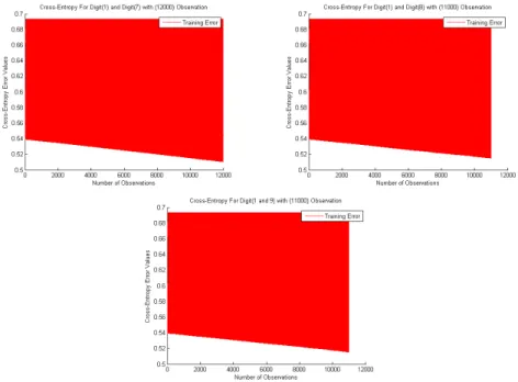
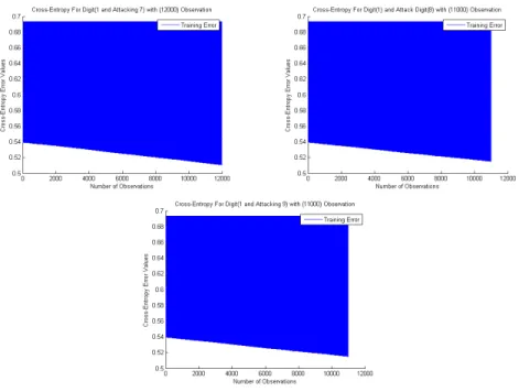
The DropConnect model has been trained using these three tampered MNIST data set. Figure 23 shows the result of our experiments.

(58)

Figure 23 shows the results of training DropConnect model on multi-run experiments using these three tampered two-class problems, which shows that the model trained well even under attacked conditions. It gave an error rate that was equal to the regular case for (1 and attack 7) as (0.4576). Moreover, it gave the same error rate for both two-class problems which are (1 and attack 8) and (1 and attack 9) as (0.4717). This is the contribution of the thesis that Deep Learning approaches can still obtain lower entropy under tampered data sets.

• Noise Two-class Problems

Evaluation of DropConnect model performance can be aected by noisy nature of data, which may aect classication error rate. There are dierent kinds of noise that can aect the images by adding some noise to their background. There have been chosen two dierent noises which were Gaussian noise and Salt and Pepper noise for this problem. Then, we added these two noises to the same two-class problems as in the previous sections. The Gaussian noise has 0 mean and 0.01 variance which is the default Gaussian noise [31]. Also, we added Salt and Pepper noise with default 0.05 noise density [31]. These two noises types have been added to the following digits (7, 8, and 9), respectively. Therefore, these classes have been shued. Moreover, DropConnect model has been trained on these three (two-class problems) in order to estimate, if the noise environ-ment can aect the performance of DropConnect algorithm or not. Also, we visualized the digits before and after adding both noises.

(59)

In the rst case, the following gures show the visualizing of digit 7 before and after adding both noises.

(a) Digit 7 (b) Gaussian Noise on Digit 7

(c) Salt and Pepper Noise on Digit 7

Figure 24. The Visualizing of Regular and Noisy Digit 7

Figure 24 shows the visualizing of regular digit 7 and after adding both noises which are Gaussian noise and Salt and Pepper noise.

Figure 25 shows the noisy digit(7) has aected the performance of DropConnect model. First plot shows the classication error of train-ing DropConnect within Gaussian noise on digit 7. Second plot shows the classication error of training DropConnect within Salt and Pepper noise on digit 7. It gave a higher error rate for Gaussian noise which was equal to (0.5164) and for Salt and Pepper noise that was equal to (0.5166). Also,

(60)

it diers in terms of over-tting problems. By adding both noise types, it causes over-tting to the classication error.

Figure 25. Training Results of DropConnect Model on Noisy Digit 7

In the second case, the following gures show the visualizing of digit 8 before and after adding both noises.

(61)

Figure 26. The Visualizing of Regular and Noisy Digit 8

Figure 27 shows the aect of the noise in digit (8) to the performance of DropConnect algorithm. First plot shows the classication error of training dropConnect within Gaussian noise on Digit 8. Second plot shows the classication error of training DropConnect within Salt and Pepper noise on digit 8. It gives lower error rate (0.5196) for Gaussian noise and (0.5197) for Salt and Pepper noise.

(62)

In the third case, the following gures show the visualizing of digit 9 before and after adding both noises.

(63)

Figure 29, shows almost the same results as in the previous two cases for noisy digits (7 and 8). First plot shows the classication error of training dropConnect within Gaussian noise on digit 9. Second plot shows the classication error of training dropConnect within Salt and Pepper noise on digit 9. It gave an error rate that was equal to (0.5201) for Gaussian noise and (0.5203) for Salt and Pepper noise. That shows that noise environment aected the performance of DropConnect algorithm by giving high error rate comparing to other cases (regular and tampered).

Last but not least, based on this section, we observed that training DropConnect under dierent attacking conditions still gave good results for the classication problem. However, noise data aected the perfor-mance of DropConnect algorithm by giving slightly higher error rate than regular and tampered data sets.

(64)

(3) Training DropConnect Model Using New Puzzle Data Set

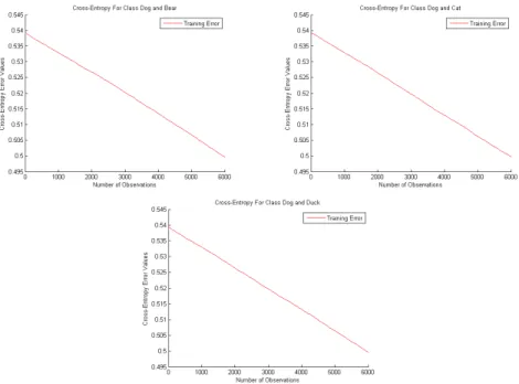
The puzzle data set contains 6 classes that represent the natural images. As we mentioned that the puzzle data set has been trained by taken two-class problems as the following, (dogs and bears), (dogs and cats), and (dogs and ducks). Each class has 3000 samples for training. The DropConnect algorithm has been trained using these three (two-class problems) and provided the following results

Figure 30. Training Results of DropConnect Model on the New Puzzle Dataset Figure 30 shows the results of training DropConnect algorithm on multi-run experiments using regular two-class problems of new puzzle data set. It shows the classication errors of training dropConnect algorithm using these two-class problems. It gave an error rate for the three cases that was equal to (0.4998). These results have been compared in chapter ve.

(65)

4.1.2. Training with Dropout

The Dropout algorithm has been trained using the same three data sets which are, toy example data set, handwritten digits data set (MNIST), and the new puzzle data set. Dropout used a Stochastic Gradient Descent to update the wright parameters. It has been used the same learning rate as in DropConnect algorithm which is, equal to (0.0001). Before training the Dropout algorithm, the data sets have been shued. The training of Dropout algorithm has been done as the

following:-(1) Training Dropout Technique using Toy Example Data Set

The toy example data set contains 100 samples divided into two classes which are, class (0) and class (1). Figure 31 shows the error rate of the training Dropout using toy example. The error rate of training Dropout using toy example was 0.2371.

(66)

(2) Training Dropout Model Using MNIST Data Set

The training of Dropout algorithm using MNIST data set has been divided into three parts as mentioned before in Dropconnect section as the

follows:-• Regular MNIST Two-class Problem

The Dropout algorithm has been trained using regular MNIST two-class problems. There have been used the same classes as in DropConnect which were (1 and 7), (1 and 8) and (1 and 9). Figure 32 shows the error rate of the training phase of those three cases.

Figure 32. Training Results of DropOut Model on Regular MNIST Dataset Figure 32 shows the results of training Dropout model with these three regular cases. It gave a higher error rate than DropConnect algorithm, for (1 and 7) it gave an error rate that was equal to (0.5105), for (1 and 8)

(67)

and (1 and 9) two-class problems, it gave an error rate that was equal to (0.5151) and (0.5154), respectively.

We have been used the same attacking mechanism that used in DropConnect algorithm. Therefore, the visualization of the regular digits and tampered digits were the same as in DropConnect algorithm's part. For this reason, We gave the direct results of the training the Dropout algorithm over these three tampered classes which were, (1 and 7), (1 and 8) and (1 and 9) with the same numbers of samples. Digit 1 has been attacked by digits (7,8, and 9). Figures 33 shows the results of the exper-iments.

(68)

Figure 33 shows the results of training Dropout model using these three tampered cases which shows that the model trained well even under attack conditions. It gives the same error rate that was equal to the regular for (1 and 7) two class problem as (0.5105). It gave lower error rate for both two class problems (1 and 8) and (1 and 9) as (0.5151). This is the contribution of the thesis that Deep Learning approaches can still obtain lower entropy under tampered data sets.

• Noise Two-class Problems

The training of Dropout algorithm using noisy two class problems followed the same procedure of DropConnect algorithm. There have been used the same two noise types which were Gaussian noise and Salt and Pepper noise with the default noise density. The visualization of the digits before and after adding the noises are the same in DropConnect section.

The Dropout algorithm has been trained over (1 and noisy 7), (1 and noisy 8) and (1 and noisy 9) and it gave the following results that are shown in gure 34.

(69)

Figure 34. Training Results of DropOut Model on Noisy MNIST Dataset Figure 34 shows the results of the training the Dropout algorithm over the three noisy two-class problems. First plot shows the classication error of the training Dropout within noisy digit 7. The second plot shows the classication error of training Dropout within noisy digit 8. The third plot shows the classication error of training Dropout within noisy digit 9. The estimated error during the training for (1 and noisy 7) was (0.5302, (1 and noisy 8) was (0.5310), and (1 and 9) was (0.5314). That shows that Dropout has been aected by noise environment which gave slightly higher error rate.

Finally, based on this section, we observed that training Dropout under dierent attacking conditions still gave good results for the classication

(70)

problem. Also, Dropout algorithm has been aected by noise data set that gave slightly higher error rate than regular and tampered data set.

(3) Training Dropout Model Using New Puzzle Data Set

The training of Dropout algorithm using two-class problems of the new puzzle data set followed the same steps of DropConnect algorithm. Figure 35 shows the results of the three cases.

Figure 35. Training Results of DropOut Model on the New Puzzle Dataset

Figure 35 shows the results of training Dropout algorithm over regular two-class problems of the new puzzle data set. In each plot, it shows the classication errors of Training Dropout over these three two-class problems. It gave error an rate for (Dog and Bear) two-class problem that was equal to (0.5250), for (Dog and Cat) as (0.5251), and for (Dog and Duck) as (0.5248).

(71)

4.1.3. Training with No-Drop

The No-Drop model has been trained using the same three data sets which are, toy example data set, handwritten digits data set (MNIST), and the new puzzle data set. It used a Stochastic Gradient Descent for back propagation step. Therefore, it used the same learning rate as in DropConnect and Dropout algorithm which is equal to (0.0001). Shuing the data set has been occurred in this technique too. The training of No-Drop algorithm has been done as the

following:-(1) Training No-Drop Technique Using Toy Example Data Set

The toy example data set has two classes which are, class (0) and class (1). Each class contains 50 samples. Figure 36 shows the error rate of the training No-Drop over toy example.

Figure 36. Error Rate of Training No-Drop Algorithm over Toy Example The error rate of training No-Drop using toy example was 0.2371 as its in Dropout algorithm.

(72)

(2) Training No-Drop Model Using MNIST Data Set

The training of No-Drop algorithm Using MNIST data set has been divided into three parts as mentioned before in Dropconnect and Dropout section as the

follows:-• Regular MNIST Two-class Problem

The No-Drop algorithm has been trained using regular MNIST two-class problems. There have been used the same classes as in DropConnect and Dropout which were (1 and 7), (1 and 8) and (1 and 9). Figure 37 shows the error rate of the training phase of those three cases.

Figure 37. Training Results of No-Drop Model on Regular MNIST Dataset Figure 37 shows the results of training No-Drop model with these three regular cases which shows that the model trained well. In each plot, we

(73)

show the classication errors of training No-Drop algorithm regular two-class problems. It gave error rate that was equal to 0.4576 for (1 and 7) two class problems, and 0.4717 for both (1 and 8) and (1 andd 9) two-class problems. It gave almost the same error rate than as in the case of training DropConnect algorithm.

We have been used the same attacking mechanism that used in DropConnect and Dropout algorithms. Therefore, the results of training the No-Drop algorithm using these three tampered classes which were, (1 and 7), (1 and 8) and (1 and 9) with the same numbers of samples. Digit 1 has been attacked by digits (7,8, and 9). Figures 38 shows the results of the experiments.