Congestion Control Algorithm
Luca De Cicco and Saverio Mascolo
Abstract—Voice over Internet Protocol (VoIP) is an Internet application of ever increasing importance. The purpose of this note is to derive a mathematical model of the Skype VoIP congestion control. The proposed model is in the form of a non linear hybrid automaton, which has been validated through extensive experiments. The dynamics of the Skype sending rate, the stability of its equilibrium points and the efficiency in bandwidth utilization while avoiding network instability are analyzed. Results show that, under network congestion, the Skype sending rate is driven by the packet loss ratio and matches the available bandwidth with a steady state finite error.
Index Terms—Hybrid automaton, Computer networks, VoIP conges-tion control
I. I
NTRODUCTIONThe transport of multimedia traffic over the Internet is of ever
increasing importance due to the spreading of multimedia content
delivery applications such as IP television (IPTV), Videoconferencing
over IP, Voice over IP (VoIP), video on demand (VoD).
The stability of the traditional data Internet is due to the
Trans-mission Control Protocol (TCP) congestion control algorithm, which
constitutes the most complex part of the TCP [1]. However, the
TCP congestion control is not appropriate to deliver time-sensitive
traffic such as VoIP calls, because of its retransmission mechanism
and additive increase multiplicative decrease (AIMD) sliding window
control [2], [3]. As a consequence, audio/video applications employ
proprietary congestion control algorithms that are executed over the
UDP protocol, which is a transport protocol that does not implement
congestion control [2].
Voice over IP is an important example of a real-time service
increasingly offered over the Internet. Skype VoIP today counts
over 40 millions active users worldwide and up to 17 millions
concurrent users
1. Skype reports that more than 100 billions minutes
of calls have been generated by Skype clients, resulting in the
most used VoIP application
2. Thus, Skype can be considered as the
most representative application producing VoIP traffic. This explosive
growth poses challenges to telecom operators and ISPs both from the
point of view of network stability and business model. For this reason,
it is important to assess the impact of a large number of Skype VoIP
calls on TCP responsive traffic that stills delivers the most part of
the Internet traffic [2], [3]. In second instance, this study is useful
to understand if there is the need for a better designed congestion
control algorithm for VoIP.
Up to now, the only congestion control algorithm for data networks
that has been widely modelled and analyzed is the standard TCP
congestion control and its variants [4],[5],[6],[7],[8]. This is due to
the fact that the TCP congestion control algorithm and its variants
are fully disclosed and well described in scientific literature and in
standardization bodies such as the IETF.
The TCP Friendly Rate Control (TFRC) protocol is a new
conges-tion control algorithm designed for multimedia flows which is under
standardization within the IETF [3]. However, as a matter of fact,
Luca De Cicco is post-doc at Dipartimento di Elettrotecnica ed Elettronica, Politecnico di Bari, Via Orabona 4, Italy (e-mail: [email protected])
Saverio Mascolo is a Faculty member of Dipartimento di Elettrotecnica ed Elettronica, Politecnico di Bari, Via Orabona 4, Italy (e-mail: [email protected]) 1http://share.skype.com/stats rss.xml 2 http://ebayinkblog.com/wp-content/uploads/2009/01/skype-fast-facts-q4-08.pdf rs(t)
Sender
Skype
Receiver
RT T(t), l(t) Emulated IP Network Congestion ControllerSkype
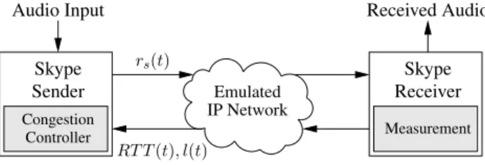
MeasurementFig. 1. Experimental testbed emulating a Skype audio call over the Internet
this standardization effort is lagging behind and TFRC is not used in
any commercial multimedia application.
The literature regarding Skype can be grouped in three main
categories: 1) studies concerning its peer-to-peer overlay network
[9], [10]; 2) studies on its traffic characteristics (see [11], [12] and
references therein); 3) studies on how to identify Skype calls among
other flows [13].
Authors of [9] present the results of a large-scale experimental
evaluation focusing on the P2P network employed by Skype. In
particular they focus on the technique employed to implement NAT
traversal functionalities and they characterize the super-nodes (SN)
of the P2P network.
In [11], [12], we have shown that Skype reacts to network
congestion by reducing the sending rate, thus being able to match
the link capacity to some extent.
In [13] the characteristics of Skype VoIP traffic have been studied
and a method to identify Skype calls among other flows has been
proposed. The method is based on two classifiers: one employs the
Chi-Square test to the payload of passively sniffed traffic, the other
measures packet size and inter packet gaps.
This paper enriches the literature by proposing for the first time
a mathematical model that describes how Skype VoIP dynamically
tracks the network available bandwidth in the presence of variable
network conditions. The model can be used to analyze fundamental
properties of the Skype congestion control such as network stability
and efficiency in network utilization.
Modelling the sending rate produced by Skype is difficult due to
the following reasons: 1) the protocol behaviour is hidden by AES
en-cryption; 2) the input variables that drive the controller are unknown;
3) it is very reasonable to conjecture that the controller implements
switching dynamics due to the use of if-then-else decisional blocks.
The rest of this note is organized as follows: in Section II
we summarize the data collected through extensive experimental
investigations in order to build the model; in Section III we propose a
mathematical model of Skype sending rate when congestion occurs;
in Section IV we derive a hybrid model of a Skype flow accessing
a bottleneck link along with a stability analysis. Finally, Section V
draws the conclusions.
II. E
XPERIMENTALT
ESTBED ANDB
ACKGROUNDFig. 1 shows a block diagram of the system to be modelled. We
consider the Skype sending rate dynamics as the output of a black box
that models the congestion controller. In [14] we have conjectured
the following two input variables: 1) the connection round trip time
(RTT); 2) the packet loss ratio. To the purpose, it is worth noting that
round trip times and packet loss rates are two variables that can be
easily measured end to be used as feedback signals in
end-to-end congestion control algorithms. In particular, congestion control
algorithms that employ delay measurements to adjust the input rate
are called
delay-based
(such as in the case of TCP Vegas and TCP
Fast), whereas algorithms that react to losses are called
loss-based
(such as in the case of TCP Reno and its variants).
Normal
S
1Losses
S
3Congestion
S
2 Li(0)=Linit ˆ l(0) = 0Fig. 2. Skype VoIP hybrid system model
The Skype VoIP sender receives round trip time
RT T
(
t
)
and loss
ratio
l
(
t
)
as feedback variables
3and set the sending rate
r
s
(
t
)
by
throttling both packet size and packet sending rate.
In order to model how feedback signals drive the Skype sending
rate, we have collected data through extensive experimental
measure-ments obtained using the testbed shown in Fig. 1, which consists of
real Skype applications running over a local area network where a
router-host is properly equipped to delay packets, set the available
bandwidth
b
(
t
)
and set packet drop probability
l
(
t
). In particular, we
have considered step-like inputs for
RT T
(
t
),
l
(
t
)
and the available
bandwidth
b
(
t
), which is a basic practice when trying to investigate
the dynamic behaviour of a system. The experimental evaluation
reported in [14] has led to the following findings: 1) variations of the
input signal
RT T
(
t
)
have no significant effect on the input rate, thus
Skype VoIP does not implement a delay-based congestion control; 2)
when the signal
l
(
t
)
is increased, Skype reacts to a persistent loss
by increasing the transmission rate; moreover, in such cases, packet
size is increased, suggesting that Skype employs a Forward Error
Correction (FEC) scheme in order to be able to recover lost packets.
FEC is a widely employed technique aimed at recovering lost packets
in real-time Internet applications such as VoIP. Basically, the idea is
to piggyback redundant information, i.e. the FEC data, on a VoIP
packet in order to be able to recover lost packets. The redundant
information is obtained by computing the XOR of previously sent
VoIP packets [15].
In [14] we have shown that the Skype VoIP sending rate can be
modelled using the
hybrid automaton
shown in Fig. 2.
In particular, the sending rate can exhibit three different dynamics
depending on the state
S
i(
i
= 1
,
2
,
3) of the automaton: in the state
S
1, which is characterized by normal network conditions, i.e. no
congestion occurs and no losses are present, the sending rate is kept
constant; in the state
S
2, which is triggered when Skype realizes that
the network available bandwidth has changed and congestion occurs,
the sending rate is throttled by using the congestion control algorithm;
in the state
S
3, which is triggered when losses not due to network
congestion are present (i.e. due to a lossy link), Skype employs a
Forward Error Correction (FEC) scheme in order to counteract the
losses attributed to a lossy link. In [14] we have found that the loss
ratio measured by Skype
ˆ
l
(
t
)
is a first-order low passed version of
the actual loss ratio
l
(
t
)
experienced by the flow. The time constant
of the filter was found to be around
11
s.
In the next Section, we will focus on the behaviour of the Skype
VoIP sending rate in the presence of variations of the available
bandwidth.
3Skype shows measured RTT and loss ratio in its “technical info” tool-tip
0 100 200 300 400 500 600 700 800 0 50 100 time (s) Throughput (kb/s)
Sending rate Loss rate Available BW
0 100 200 300 400 500 600 700 800 0 50 100 150 time (s)
Packet Sending rate (packets/s)
0 100 200 300 400 500 600 700 800 0 100 200 300 400 500 time (s)
Packet Size (byte)
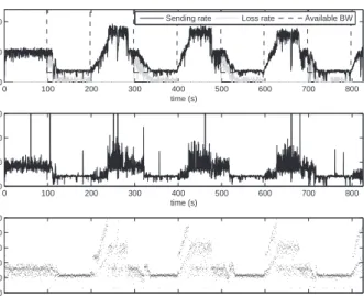
Fig. 3. Sending rate, loss rate, packet sending rate and packet size evolution in the presence of a square wave available bandwidth of200s period
III. T
HES
KYPEC
ONGESTIONC
ONTROLM
ODELThis Section aims at providing a mathematical model describing
the dynamic behaviour of the Skype sending rate in the presence of
a variable link available bandwidth.
To the purpose, we investigate how the Skype sending rate reacts
to sudden changes of available bandwidth. We employ an available
bandwidth that varies as a square wave with maximum value
A
M=
160
kb/s, minimum value
A
m= 16
kb/s and with a period equal to
200
s, which is large enough to show all the transient dynamics.
Fig. 3 shows that Skype decreases the sending rate when the link
capacity drops from the value
A
Mto the value
A
m. The Skype
flow takes approximately
40
s to track the available bandwidth during
which it experiences a significant loss rate. It can be viewed that,
when the available bandwidth drops, the loss rate increases to a peak
value of
35
kb/s whereas the sending rate reduces to less than
20
kb/s
in around
40
s. When the link capacity increases (i.e. at
t
= 400
s)
the input rate ramps up to
90
kb/s, again in around
40
s.
In order to find out the Skype controller dynamics, we have
captured both packet sizes and packet sending rate over time (see
Fig. 3). It can be noticed that the packet sending rate drops in a
step-like function when Skype detects congestion, whereas the packet size
is decreased slowly, resulting in a slow adaptation to the available
bandwidth. In other terms, the most part of Skype congestion control
is performed by throttling the packet sending rate, whereas the packet
size is changed for fine tuning.
Based on the large number of experiments we have run [11],
[14], we make the hypothesis that the audio codec employed by
Skype is multi-rate so that the encoder can select among
N
levels
L
k=
{
L
1, L
2, . . . , L
N}
with
L
1< L
2<
· · ·
< L
N. Moreover,
we assume that the Skype adaptive codec is able to select the most
appropriate mode according to a metric which is the analogous of
Carrier to Interference ratio (C/I) in the case of Adaptive Multi-Rate
Wide Band (AMR-WB) encoder.
By letting
i
(
t
)
denote the switching law
i
(
·
) :
R
7→ {
1
, . . . , N
}
and
L
i(t)the encoder level at time
t
, we are ready to make the key
hypothesis that the Skype control law for the sending rate is ruled
by the following equation:
r
s(
t
) = (1
−
ˆ
l
(
t
))
·
(1 +
f
(
t
))
L
i(t)(1)
where
f
:
R
7→
[0
,
1]
⊂
R
models the FEC action, meaning that
when
f
(
t
) = 0
the FEC action is not active whereas when
f
(
t
) = 1
0 0 0.5 1 200 400 600 800 1000 1200 1400 0 200 400 600 800 1000 1200 1400 0 500 0 200 400 600 800 1000 1200 1400 200 1 0 0.5 1.5 0 0 50 150 100 400 600 800 1000 1200 1400 Av. Bandwidth Predicted thr. Actual thr.
Packet size (bytes)
Loss ratio kb/s f ( t ) l(t) ˆl(t) t(s)
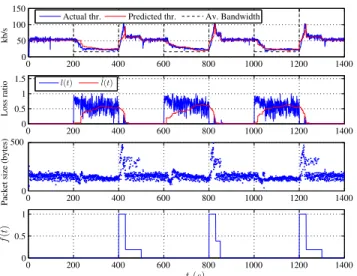
Fig. 4. Comparison between the actual and predicted rate using (1)
the FEC action is at maximum. Equation (1) describes the following
behaviours: when
ˆ
l
(
t
) = 0
(i.e. no congestion occurs) the sending
rate
r
s(
t
)
is given by
L
i(t)or
(1 +
f
(
t
))
L
i(t)if the FEC is active.
When congestion happens (i.e.
ˆ
l
(
t
)
6
= 0) the feedback signal reduces
the sending rate of
ˆ
l
(
t
)(1 +
f
(
t
))
L
i(t).
We have run a set of experiments using a square wave available
bandwidth with maximum value of
160
kb/s, a minimum value of
16
kb/s with a period of
400
s.
Fig. 4 shows that the packet size is kept roughly constant until the
first bandwidth increase occurring at
t
= 400
s. We conjecture that
Skype infers an increase of the available bandwidth by measuring
a decrease in both RTT and
l
(
t
), which triggers a “probing phase”.
Since losses can occur during this phase, Skype activates the FEC
action. We conjecture that Skype implements the FEC action by
bundling multiple frames in a single packet, so that an increase in the
FEC action will turn into a larger packet size [12], [15]. For these
considerations, we conjecture the FEC action
f
(
t
)
shown in Fig. 4,
which is proportional to the packet size. Fig. 4 shows that the FEC
action is reduced when the filtered loss ratio
ˆ
l
(
t
)
reaches zero, and
it is turned off later when
ˆ
l
(
t
)
is detected not to grow. Moreover, by
looking at the packet size evolution, we infer that the FEC action is
kept off during congestion.
Fig. 4 shows both the Skype measured and predicted sending rate
using (1) with a constant value of
L
i(t)equal to
56
kb/s. This value
is measured at the beginning of the Skype connection when
f
(
t
) = 0
and
ˆ
l
(
t
) = 0.
Equation (1) nicely predicts the Skype sending rate, both in the case
of presence or absence of congestion, including the large transient
time we have reported before.
In conclusion, the main driver of the Skype sending rate is
ˆ
l
(
t
),
which is a low-pass filtered version of the actual loss ratio
l
(
t
).
Therefore, the dynamics of
ˆ
l
(
t
)
affects the sending rate response
to congestion which is somewhat slow.
IV. H
YBRIDA
UTOMATON MODELLING AS
KYPEF
LOWA
CCESSING AB
OTTLENECKIn this Section we propose a hybrid automaton to model a Skype
flow accessing a single bottleneck link characterized by an available
bandwidth
b
(
t
), a drop tail queue whose maximum size is
q
Mand a
round trip time
T
which is the sum of the delay of the forward path
T
1and the delay of the backward path
T
2.
˙
q
= 0
Σ
1o
= 0
˙
q
=
r
−
b
˙ˆ
l
=
f
2Σ
2˙
q
= 0
Σ
3o
= 0
o
=
r
−
b
r > b q= 0 r < b q6= 0, q6=qM r≤b q=qM˙ˆ
l
=
f
2l
˙ˆ
=
f
1 r≥bFig. 5. The hybrid automaton modelHof a Skype flow accessing a drop tail queue
The queue dynamics can be modelled by the following differential
equation [16]:
˙
q
(
t
) =
(
0
q
(
t
) = 0
, r
(
t
)
≤
b
(
t
)
or
q
(
t
) =
q
M, r
(
t
)
≥
b
(
t
)
r
(
t
)
−
b
(
t
)
otherwise
(2)
where
r
(
t
)
is the queue input rate. The queue overflow rate
o
(
t
)
can
be modelled as follows:
o
(
t
) =
r
(
t
)
−
b
(
t
)
q
(
t
) =
q
M, r
(
t
)
> b
(
t
)
0
otherwise
(3)
which means that when the queue is full the exceeding input rate
r
(
t
)
−
b
(
t
)
is dropped [16].
The dynamic model of the Skype sending rate can be derived from
(1) by considering that the feedback signal
ˆ
l
(
t
)
is a filtered version of
the actual packet loss ratio
l
(
t
) =
o
(
t
)
/r
(
t
)
measured at the sender
after the backward delay
T
2. Based upon experiments, we assume
that Skype filters
l
(
t
−
T
2)
using a first order low pass filter with a
time constant
τ
:
˙ˆ
l
(
t
) =
−
1
τ
ˆ
l
(
t
) +
1
τ
l
(
t
−
T
2)
which, by considering that
l
(
t
) =
o
(
t
)
/r
(
t
), turns out:
˙ˆ
l
(
t
) =
−
1
τ
ˆ
l
(
t
) +
1
τ
o
(
t
−
T
2)
r
(
t
−
T
2)
(4)
By substituting (1) and (3) in (4), after straightforward
computa-tions we obtain:
˙ˆ
l
(
t
) =
f
1=
1 −ˆl(t) τ−
b(t−T2)/τ (1−ˆl(t−T2))(1+f(t−T2))Li(t−T2 )q
=
q
M,
r > b
f
2=
−
1τˆ
l
(
t
)
otherwise
(5)
It is simple to show that the dynamics of the considered system can
be described by means of the three states hybrid automaton
H
which
is shown in Fig. 5.
Let
X
=
{
ˆ
l, q
: 0
≤
ˆ
l
≤
1
,
0
≤
q
≤
q
M} ⊂
R
2be the set of
continuous states,
x
(
t
) =
[ˆ
l
(
t
)
q
(
t
)]
T∈
X
be the continuous
state of the system at the continuous time
t
and
Σ =
{
Σ
1,
Σ
2,
Σ
3}
denote the discrete set of
H
[17]. In particular: the state
Σ
1holds
when the queue is empty and the input rate is less then or equal
to the link available bandwidth; the system dynamics is described
by state
Σ
2when the queue is neither full nor empty; the state
Σ
3describes the evolution of the system when the queue is full and the
input rate is greater than or equal to the available bandwidth [16].
By considering the guard conditions (
r > b
and
r < b
) the domains
(or invariant sets) of the three discrete states are the following:
Dom
(Σ
1)
=
{
x
∈
X
|
q
= 0
∧
1
−
b
(1 +
f
)
L
i≤
ˆ
l
≤
1
}
Dom
(Σ
3)
=
{
x
∈
X
|
q
=
q
M∧
0
≤
ˆ
l
≤
1
−
b
(1 +
f
)
L
i}
In the sequel we will prove four lemmas that will be used to
analyze the stability of the equilibrium points of the automaton
H
.
Before starting to prove the first Lemma, we notice that the filter
time constant
τ
∼
= 11
s is from
10
up to
100
times the value
of the
RT T
measured in realistic Internet scenario, which goes
from milliseconds up to few seconds such as in the case of old
wireless GPRS networks or satellite connections. Moreover,
ITU-T recommends a maximum value of
400
ms for mouth-to-ear delay
[18], which corresponds to a round trip time of
800
ms, in order
to consider the quality of a VoIP call acceptable. Therefore, since
τ
T
2it is well justified to neglect the time delay
T
2in the model
of the system.
Lemma 1:
When the automaton is in the state
Σ
3, the following
inequality holds:
b
(
t
)
≤
L
i(t)(1 +
f
(
t
))
(6)
Proof:
In the state
Σ
3,
b
(
t
)
≤
r
(
t
)
holds. Since
r
(
t
) = (1
−
ˆ
l
(
t
))
L
i(t)(1 +
f
(
t
))
≤
L
i(t)(1 +
f
(
t
)), the inequality (6) is proved.
Thus, if (6) is not verified
Dom
(Σ
3)
is an empty set, and
Σ
3is not
reachable.
Lemma 2:
The system
Σ
3has a unique asymptotically stable
equilibrium point that is feasible:
ˆ
l
∗= 1
−
q
b∗L∗(1+f∗)
q
∗=
q
M(7)
where
b
∗,
L
∗,
f
∗are the inputs at steady state.
Proof:
The state
Σ
3holds when
r
(
t
)
≥
b
(
t
)
and the queue is full
(
q
=
q
M), i.e. when congestion occurs. Equation (5) in steady state
condition (i.e. when
l
˙ˆ
(
t
) = 0
and
q
˙
(
t
) = 0) gives the equilibrium
point (7) where
b
∗,
L
∗and
f
∗are the steady state inputs. Since
from Lemma 1 when in
Σ
3it holds
b
∗≤
L
∗(1 +
f
∗), it results that
ˆ
l
∗∈
[0
,
1], i.e. the equilibrium is feasible.
In order to prove the stability of the equilibrium, we employ the
direct Lyapunov method. By using the candidate Lyapunov function
V
(ˆ
l
) =
12
(ˆ
l
−
ˆ
l
∗
)
2the following derivative of
V
˙
(ˆ
l
)
is obtained after
straightforward computations:
˙
V
(ˆ
l
) =
−
1
τ
(ˆ
l
−
ˆ
l
∗)
2(2
−
ˆ
l
−
ˆ
l
∗)
1
−
ˆ
l
which is definite negative for all
ˆ
l
∈
[0
,
1]. Thus, for the direct
Lyapunov stability criterion the equilibrium
ˆ
l
∗is asymptotically
stable.
Lemma 3:
The system
Σ
1has a unique equilibrium point:
ˆ
l
∗= 0
q
∗= 0
(8)
which is globally asymptotically stable.
Proof:
The lemma is proved by observing that
Σ
1is a linear
system with one real strictly negative eigenvalue.
Lemma 4:
The hybrid automaton
H
has a sink state
Σ
3if
b
∗<
(1 +
f
∗)
L
∗and a sink state
Σ
1if
b
∗>
(1 +
f
∗)
L
∗.
Proof:
Let us consider the first part of the proposition which
assumes
b
∗<
(1 +
f
∗)
L
∗. The proof starts by showing that for
any initial condition
(ˆ
l
0, q
0)
∈
X
, the state dynamics of the hybrid
automaton enters the state
Σ
3and remains indefinitely in this state,
i.e.
Σ
3is a
sink
state. To this purpose we find the reachability set of
H
.
Fig. 6 (a) shows that
Dom
(Σ
2)
is partitioned in the following two
zones depending on the sign of
q
˙
:
Z
1=
{
x
∈
X
: ˆ
l <
1
−
b
∗/
(1 +
f
∗)
L
∗,
0
≤
q < q
M}
Z
2=
{
x
∈
X
: ˆ
l >
1
−
b
∗/
(1 +
f
∗)
L
∗,
0
< q
≤
q
M}
1 ˙ q <0 Dom(Σ2) ˙ˆ l <0 r < b (a) ˆ l∗ (b) Dom(Σ3) 1 Dom(Σ1) Dom(Σ1) ˆl ˆl q qM q qM 1− b∗ (1+f∗)L∗ P Z1 Z2 (r > b) (r < b)Fig. 6. Qualitative phase portrait of the Skype state space model when (a)
b∗<(1 +f∗)L∗or (b)b∗≥(1 +f∗)L∗
Thus, it results that if
r > b
,
x
∈
Z
1then the queue builds up
otherwise
x
∈
Z
2and the queue is drained.
It is easy to show that if we initialize
H
in the state
Σ
1(the queue
is empty and
r < b
) then from (5) the state evolution is given by:
ˆ
l
(
t
) = ˆ
l
0e
−t τ
q
(
t
) = 0
where the initial condition is
x
0= (ˆ
l
0,
0)
∈
Dom
(Σ
1). The state
of
H
remains in
Σ
1if
r
(
t
)
< b
(
t
)
(i.e. when
ˆ
l
(
t
)
>
1
−
b
∗/
(1 +
f
∗)
L
∗). The state switches to
Σ
2at the time
t
12when the sending
rate matches the available bandwidth, i.e. when
r
(
t
12) =
b
∗:
t
12=
−
τ
log
1
ˆ
l
0(1
−
b
∗(1 +
f
∗)
L
∗)
that is positive for each
x
0∈
Dom
(Σ
1). Thus, we can conclude
that if we initialize
H
in the
Σ
1state, the only reachable state is
Σ
2after a time
t
12. Moreover, since the state is now in the region
Z
1the queue must build up, so that the only reachable state from
Σ
2is now
Σ
3. Thus, we can conclude that if
H
is initialized in
Σ
1the
only possible evolution of the state is
Σ
1→
Σ
2→
Σ
3.
Let us now focus on the states that can be reached by initializing
H
in
Σ
2, that is
(ˆ
l
0, q
0)
∈
Dom
(Σ
2) =
Z
1∪
Z
2. By solving (5),
for
t >
0
the evolution of the state is given by:
ˆ
l
(
t
) = ˆ
l
0e
−t τ(9)
q
(
t
) =
q
0−
ˆ
l
0τ L
∗(1 +
f
∗)(1
−
e
− t τ) + (
L
∗(1 +
f
∗)
−
b
∗)
t
(10)
It is easy to show that if the initial condition belongs to
Z
1, there is
no way for the state to end in
Σ
1(since the queue must build up) so
that the only state that can be reached is
Σ
3(full queue). Let us now
start from the initial condition in
Z
2. Now two different evolutions
of the hybrid automaton are possible: the state can either go in
Σ
1,
then back to
Σ
2and then to
Σ
3, or either go directly in
Σ
3. Finally,
if the initial condition belongs to the set:
P
=
{
x
∈
Z
2:
q < τ
(
L
∗(1 +
f
∗)
−
b
∗) log
1
−
b
∗L
∗(1 +
f
∗)
+
τ L
∗(1 +
f
∗)ˆ
l
−
τ
(
L
∗(1 +
f
∗)
−
b
∗)(1 + log ˆ
l
)
} ⊂
Z
2the state will follow the path
Σ
2→
Σ
1→
Σ
2→
Σ
3, otherwise
it will follow the path
Σ
2→
Σ
3. In either the cases if the hybrid
automaton starts from
Σ
2the state will end in
Σ
3that is, the queue
fills up and packet losses occur.
In order to conclude the first part of the proof we need to show that
if we initialize the system in
Σ
3the state of
H
will remain in
Σ
3. This
follows from Lemma 2 since the equilibrium (7) is asymptotically
stable.
100 90 80 70 60 50 40 30 20 10 0.1 0.2 0.3 0.4 0.5 0.6 0.7 0.8 0.9 0 1 q (ˆl∗, q∗) = (0.2546, qM) ˆ l Fig. 7. Trajectories obtained using the proposed model whenL∗= 54kb/s andb∗= 30kb/s
The second part of the proof which states that
Σ
1is a sink state
if
b
∗>
(1 +
f
∗)
L
∗follows the same arguments we have developed
in the first part and it is omitted due to space limitation.
Proposition 1:
By considering the equilibrium inputs
b
∗,
L
∗and
f
∗, the hybrid automaton shown in Fig. 5 reaches the following
asymptotically stable equilibrium state:
ˆ
l
∗= 1
−
q
b∗ L∗(1+f∗)q
∗=
q
M(11)
if
b
∗<
(1 +
f
∗)
L
∗or:
ˆ
l
∗= 0;
q
∗= 0
(12)
otherwise.
Proof:
From Lemma 4 we know that if
b
∗<
(1 +
f
∗)
L
∗then
Σ
3is a sink state, so that for any initial condition
(ˆ
l
0, q
0)
∈
X
the
state ends in
Σ
3. Moreover, in Lemma 2 we have proved that
Σ
3has
the asymptotic stable equilibrium (11), so that we can conclude that
for any initial condition
(ˆ
l
0, q
0)
∈
X
the state will asymptotically
converge to (11).
If we assume
b
∗>
(1+
f
∗)
L
∗, by following similar arguments, we
can conclude that for any
(ˆ
l
0, q
0)
∈
X
the state will asymptotically
converge to (12).
Fig. 7 shows the trajectories obtained by considering initial conditions
(marked with a
×
)
(ˆ
l
0, q
0)
∈
X
. The figure shows that all the
trajectories are attracted by the stable equilibrium
(ˆ
l
∗, q
∗)
predicted
by Proposition 1 and marked in Fig. 7 with a
◦
.
Proposition 2:
Under network congestion, i.e.
r
∗> b
∗, the Skype
controller produces a steady state overflow rate equal to:
o
∗=
p
b
∗L
∗(1 +
f
∗)
−
b
∗(13)
which means that Skype is not able to avoid congestion.
Proof:
Being in
Σ
3, Lemma 1 implies
b
∗<
(1 +
f
∗)
L
∗.
From Proposition 1 we know that (11) is an asymptotically stable
equilibrium for
H
. Therefore, by considering (3), the steady state
value of the overflow rate is given by:
o
∗= (1
−
ˆ
l
∗)
L
∗(1 +
f
∗)
−
b
∗(14)
Now by substituting (11) in (14), it turns out (13). The overflow rate
o
∗is greater than zero since
b
∗< L
∗(1 +
f
∗). In other terms, under
congestion, the evolution of the system will be described by
Σ
3(see
b(t) 50 100 150 0 0 20 200 250 300 350 400 40 80 60 20 0 0 50 100 150 200 250 300 350 400 400 350 300 250 200 150 100 50 0 0 40 Actual rate b∗= 30 kb/s ;L∗= 56 kb/s qM o∗∼= 11kb/s 10 5 q ( t ) (KB) o ( t ) (kb/s) r ( t ) (kb/s) t(s) r∗∼= 41kb/s
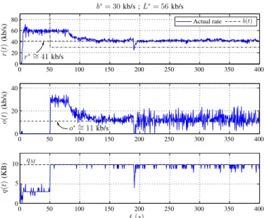
Fig. 8. Validation of the Skype VoIP model (Propositions 1 and 2)
Lemma 4), thus the queue will be full (
q
∗=
q
M) and the overflow
rate will be persistent (
o
∗>
0).
In order to validate this Proposition through an experiment, a Skype
flow has been injected in a bottleneck whose maximum queue length
is
q
M= 10
KB and that experiences an available bandwidth drop
from
120
kb/s to
b
∗= 30
kb
/s
at
t
= 50
s.
Fig. 8 shows the results of the experiment. The actual throughput,
the loss rate and the queue length produced by the Skype flow are
compared with the steady state values (represented in dashed thick
lines in Fig. 8) predicted by the model. It is worth noting that the
throughput at equilibrium (
r
∗= (1
−
ˆ
l
∗)
L
∗'
40
.
988
kb/s) and
the loss rate (
o
∗=
√
b
∗L
∗−
b
∗∼
= 10
.
988
kb/s) found by using
Propositions 1 and 2 nicely match the steady state values measured
through the experiment.
V. C
ONCLUSIONSIn this note we have proposed a hybrid automaton to model
the congestion control algorithm implemented by the Skype VoIP
application. Main findings are: 1) the loss ratio is the main driver
of the Skype input rate; 2) the sending rate matches the available
bandwidth with a finite error, so that Skype experiences a persistent
congestion; 3) the sending rate matches the available bandwidth with
a slow time constant.
R
EFERENCES[1] V. Jacobson, “Congestion avoidance and control,”ACM Comput. Com-mun. Rev., vol. 18, no. 4, pp. 314–329, 1988.
[2] L. Eggert and G. Fairhurst, “UDP Usage Guidelines for Application Designers,”RFC 5405, Nov. 2008.
[3] S. Floyd, M. Handley, J. Padhye, and J. Widmer, “Equation-based con-gestion control for unicast applications,” inProc. of ACM SIGCOMM, 2000.
[4] S. Low, F. Paganini, and J. Doyle, “Internet congestion control,”IEEE Control Systems Magazine, vol. 22, no. 1, pp. 28–43, 2002.
[5] J. Lee, S. Bohacek, J. P. Hespanha, and K. Obraczka, “Modeling communication networks with hybrid systems,”IEEE/ACM Transactions on Networking, vol. 15, no. 3, pp. 630–643, 2007.
[6] S. Mascolo, “Congestion control in high-speed communication networks using the Smith principle,” Special Issue on “Control methods for communication networks” Automatica, vol. 35, no. 12, pp. 1921–1935, 1999.
[7] C. Hollot, V. Misra, D. Towsley, and W. Gong, “Analysis and design of controllers for AQM routers supporting TCP flows,”IEEE Transactions on Automatic Control, vol. 47, no. 6, pp. 945–959, 2002.
[8] R. Srikant, The Mathematics of Internet Congestion Control. Birkh¨auser, 2004.
[9] S. Guha, N. Daswani, and R. Jain, “An Experimental Study of the Skype Peer-to-Peer VoIP System,” inProc. IPTPS ’06, Feb. 2006.
[10] S. Baset and H. Schulzrinne, “An Analysis of the Skype Peer-to-Peer Internet Telephony Protocol,” inProc. of IEEE INFOCOM ’06, Apr. 2006.
[11] L. De Cicco, S. Mascolo, and V. Palmisano, “An Experimental Investi-gation of the Congestion Control Used by Skype VoIP,” inProc. of 5th International Conference on Wired/Wireless Internet Communications (WWIC), Coimbra, Portugal, May 2007.
[12] ——, “Skype Video Responsiveness to Bandwidth Variations,” inProc. of ACM NOSSDAV 2008, Braunschweig, Germany, May 28–30, 2008. [13] D. Bonfiglio, M. Mellia, M. Meo, D. Rossi, and P. Tofanelli, “Revealing
skype traffic: when randomness plays with you,” in Proc. of ACM SIGCOMM ’07, Aug. 2007.
[14] L. De Cicco, S. Mascolo, and V. Palmisano, “A Mathematical Model of the Skype VoIP Congestion Control Algorithm,” inProc. of IEEE Conference on Decision and Control ’08, Cancun, Mexico, 9-11 Dec 2008.
[15] W. Jiang and H. Schulzrinne, “Comparison and optimization of packet loss repair methods on voip perceived quality under bursty loss,” inProc of NOSSDAV ’02, Miami, Florida, USA, 2002.
[16] S. Mascolo, “Modeling the Internet congestion control using a Smith controller with input shaping,” Control Engineering Practice, vol. 14, no. 4, pp. 425–435, Apr. 2006.
[17] J. Lygeros, K. Johansson, S. Simic, J. Zhang, and S. Sastry, “Dynam-ical properties of hybrid automata,”IEEE Transactions on Automatic Control, vol. 48, no. 1, pp. 2–17, 2003.