Optimizing Network Performance In Replicated Hosting
Ningning Hu
†Oliver Spatscheck
§Jia Wang
§Peter Steenkiste
††
Carnegie Mellon University, Pittsburgh, PA 15213, USA
§
AT&T Labs – Research, Florham Park, NJ 07932, USA
Abstract
Most important commercial Web sites maintain multiple replicas of their server infrastructure to increase both reli-ability and performance. In this paper, we study how many replicas should be used and where they should be placed in order to improve client network performance, including both the latency (e.g., round-trip time) between clients and the replicas, and the bandwidth performance between them. This study is based on a large scale measurement study from an 18-node infrastructure, which reveals for the first time the distribution of today’s Internet end-user access band-width. For example, we find that 50% of end users have access bandwidth less than 4.2Mbps. Using a greedy algo-rithm, we show that the first five replicas dominate latency optimization in our measurement infrastructure, while the first two replicas dominate bandwidth optimization. We also found that geographic diversity does not help as much for bandwidth optimization as it does for latency. To determine the proper trade-off between latency and bandwidth, we use a simplified TCP model to show that, when content size is less than 10KB, the deployment should focus on optimizing latency, while for content sizes larger than 1MB, the deploy-ment should focus on optimizing bandwidth.
1
Introduction
It is increasingly common for content providers to use replication to increase the reliability and performance of their server infrastructure. Some content providers use commercial Content Distribution Networks (CDNs) [22] to achieve this goal, while others replicate their server infras-tructure in multiple locations. Most large content providers use both techniques depending on the type and the value of the content delivered. In this paper, we focus on the latter method, i.e., replicating the whole server infrastruc-ture. This technique has two advantages over CDNs. First, replicating the entire server infrastructure (we will call each replicated server a replica) at multiple sites not only
al-lows the content to be delivered from multiple locations, but also allows the content provider to perform more compli-cated tasks such as securing e-commerce transactions which require real time database access. Second, unlike CDNs which require a master server as the content origin, replicas allow the content provider to operate seamlessly if one of its replicas is not available.
In this paper we focus on how replication can improve performance. The most direct metric for optimizing con-tent replications is concon-tent download time. However, it is impossible to measure download time from a collection of possible replicas toeveryclient on the Internet. To address this problem, multiple solutions have been proposed includ-ing the use of geographic location [19], network mappinclud-ing services [7], and network hops and latency [6, 23, 4, 18]. In this paper, we estimate the download time for objects of var-ious sizes by measuring the round-trip time (RTT) and the available bandwidth to each prefix using Pathneck [8]. In our optimization, we consider both the overall performance and the performance of the 20% worst destinations.
Our contributions are four-fold. First, we show that most hosts access the Internet through relatively low bandwidth links and for these hosts, replica selection based on band-width has no benefit. Second, for well-provisioned hosts, the first two replicas provide most of the improvement that can be gained from bandwidth optimization, while we will need five replicas for RTT optimization. Third, we demon-strate that replica placement to optimize bandwidth does not follow a clear geographic pattern, while RTT optimization does. Fourth, we use a simple TCP data transmission model to show that when the content size is less than 10KB, the replica deployment should minimize RTT; when the content size is larger than 1MB, the deployment should maximize bandwidth.
The remainder of the paper is structured as follows. We describe our measurement methodology in Section 2, and summarize our measurement results in Section 3. We then present the results of both bandwidth and RTT optimization under different application scenarios in Section 4. Section 5 uses a simplified TCP model to evaluate the trade-off
be-2
1 15 15 2 1
measurement
packets measurementpackets
60B
60 packets load packets
255 255 255
500B TTL 30 packets
ICMP ECHO packet
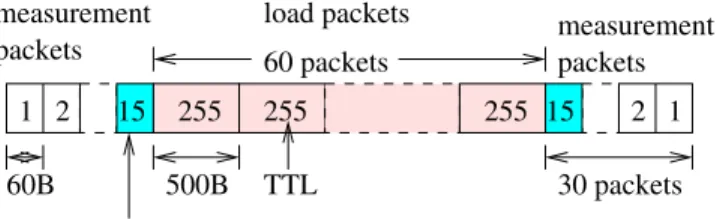
Figure 1. Probing packet train of the modified Pathneck
tween RTT and bandwidth optimization. Finally, we present the related work in Section 6 and conclude in Section 7.
2
Methodology
In this section, we first briefly review the measurement tool that we used. We then describe our measurement in-frastructure followed by a discussion of the implications of our methodology.
2.1
Measurement Tool–Pathneck
Our measurement data was obtained using Pathneck [8], which is an active probing tool that allows end users to ef-ficiently and accurately locate bottleneck links on the In-ternet. Pathneck is based on a novel way of construct-ing a probconstruct-ing packet train–Recursive Packet Train, which combines load packets and measurement packets. The load packets interleave with background traffic, which affects the length of the Pathneck train. The change in train length pro-vides information about the available bandwidth on a link. The measurement packets have carefully controlled TTL values, so that the ICMP packets generated when packets expire can be used by the source to estimate the length of the train at every hop in the network path. Pathneck can estimate the bottleneck location and an upperbound on the available bandwidth on the bottleneck link (and thus the path). Similar to traceroute, it also measures the route and the RTT. Details on Pathneck can be found elsewhere [8].
A problem with the original Pathneck tool is that it can-not measure the last hop of Internet paths, which are good candidate bottlenecks. For our measurement, we modified the Pathneck tool to alleviate this problem. The idea1 is to
use ICMP ECHO packets instead of UDP packets as the measurement packets for the last hop. For example, the packet train in Figure 1 is used to measure a 15-hop path. If the destination replies to the ICMP ECHO packet, we can
1It was originally suggested by Tom Killlian from AT&T Labs–
Research.
Table 1. Measurement source nodes
ID Location ID Location ID Location
S01 US-NE S07 US-SW S13 US-NM
S02 US-SM S08 US-MM S14 US-NE
S03 US-SW S09 US-NE S15 Europe
S04 US-MW S10 US-NW S16 Europe
S05 US-SM S11 US-NM S17 Europe
S06 US-SE S12 US-NE S18 East-Asia NE: northeast, NW: northwest, SE: southeast, SW: southwest ME: middle-east, MW: middle-west, MM: middle-middle
obtain the gap value on the last hop. In order to know where the ICMP packets should be inserted in the probing packet train, Pathneck first uses traceroute to get the path length. Note that this Pathneck modification works only for Inter-net destinations that reply to ICMP ECHO packets.
2.2
Measurement Infrastructure
In our measurement, we used 18 measurement sources (Table 1), 14 of which are in the US, 3 are in Europe, and 1 is in East-Asia. All the sources directly connect to a large Tier-1 ISP (referred asX) via 100Mbps Ethernet links. In this paper, we consider these 18 sources as the candidate locations that an application can use to replicate its server infrastructure. In the rest of this paper, we also refer to these sources asreplicas.
The measurement destinations are selected as follows. Our goal is to cover as many diverse locations on the In-ternet as possible. We select one IP address as the mea-surement destination from each of the 164,130 prefixes ex-tracted from a BGP table. Ideally, the destination should correspond to an online host that replies to ping packets. However it is difficult to identify online hosts without prob-ing them. In our study, we partially alleviate this problem by picking IP addresses from three pools of existing data sets collected by the ISP: Netflow traces, client IP addresses of some Web sites, and the IP addresses of a large set of local DNS servers. That is, for each prefix, whenever possible, we use one of the IP addresses from those three sources in that prefix; otherwise, we randomly pick an IP address from that prefix. In this way, we are able to find reachable desti-nation in 67,271 of the total 164,130 prefixes.
We collected Pathneck data from the 18 sources to the 164,130 selected destinations from August 28, 2004 to September 30, 2004. Note that for those unreachable des-tinations, we only have partial path information. Ideally, the partial paths would connect the measurement sources to a commonjoin nodethat is the last traced hop from each source, so the join node stands in for the destination in a consistent way. Unfortunately, such a join node may not
exist, either because there may not be a node shared by all the 18 measurement sources to a given destination or the shared hop may not be the last traced hop. For this reason, we relax the constraints for the join node: the join node only needs to be shared by 14 measurement sources, and it need only be within three hops from the last traced hop. Here “14” is simply a reasonably large number that we choose. This allows us to make the best of the available data while still having comparable data. Specifically, this allows us to include over 141K destinations (86% of the total) in our analysis, among which 47% are real destinations, and 53% are join nodes. We refer to these 141K destinations asvalid destinations.
2.3
Applicability to Other ISPs
Since all our measurement sources are connected to the same ISPX, our analysis results could easily be specific to ISPX. However, we believe that the results are more broadly applicable. The intuition is that the widely used “hot-potato” routing approach forces packets to quickly en-ter other ISPs’ networks if they need to traverse those net-works to reach their destinations. For those packets, the time spent in ISPXis very small. Since ISPX is very well engineered and its links rarely appear as bottlenecks in our measurements, ISPXis largely “transparent” in these cases and our measurement sources can be considered as reason-able vantage points for those ISPs.
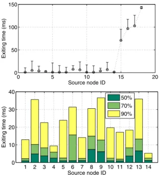
To validate this intuition, we pick 7 top Tier-1 ISPs peer-ing with ISPXfrom Keynote [3]; 5 of the ISPs are in the US and 2 are in Europe. 64% of all the paths enter these ISPs directly from ISPX. Figure 2 shows the time spent within
X(referred asexit time) by the packets on those paths. The top graph shows the median (middle circle), 10th percentile (bottom bar, generally overlapped with the circle), and 90th percentile (top bar) values of the exit time for all the mea-surement sources. It is not surprising thatS15,S16,S17, andS18have large exit times since they are in Europe or East-Asia, and have to use the trans-atlantic/pacific links to reach the peering points. The bottom graph shows the me-dian, 70th percentile, and 90th percentile values of the exit time distributions for the 14 measurement sources located in the US. For each measurement source, over 70% of the paths have exit times less than15ms; most of them are less than 10ms. The small exit times confirm our claim that our measurement setup and the corresponding analysis are also useful for the scenario where the replicas are located at sources connected to other major Tier-1 ISPs, and the scenario where the whole replicated service is located at a source which multihomes to all major Tier-1 ISPs.
0 5 10 15 20 0 50 100 150 Source node ID Exiting time (ms) 1 2 3 4 5 6 7 8 9 10 11 12 13 14 0 10 20 30 40 Source node ID Exiting time (ms) 50% 70% 90%
Figure 2. The exit times to neighbor ISPs.
3
Performance of Individual Replica
In this section, we look at the RTT and bandwidth per-formance from each individual replica to all destinations to understand their potential in improving RTT and bandwidth performance.
3.1
RTT Performance
Figure 3 shows the cumulative distribution (CDF) of RTT measurements from individual replicas. For the sake of clarity, we only plot the measurements for three repli-cas: S01,S17, and S18, which are in the United States, Europe, and East Asia, respectively. The curve labeled with “best” corresponds to the optimal performance using all 18 replicas, i.e., the smallest RTT from all 18 replicas. We can see that RTT can be significantly improved by using multi-ple replicas. In addition, the performance of using a single replica varies depending on its location. These results show how the physical location of replicas plays an important role in RTT optimization.
3.2
Bandwidth Performance
Figure 4 illustrates the cumulative distributions of band-width measurements. Because Pathneck only provides an upper-bound of path available bandwidth, the bandwidth distributions shown in Figure 4 are upper-bounds for the ac-tual bandwidth distributions. Compared with Figure 3, we
0 50 100 150 200 250 300 350 400 0 0.1 0.2 0.3 0.4 0.5 0.6 0.7 0.8 0.9 1 best S01 S17 S18
round trip time (ms)
CDF
Figure 3. RTT performances from individual replicas 0 10 20 30 40 50 60 0 0.1 0.2 0.3 0.4 0.5 0.6 0.7 0.8 0.9 1 best S01 S17 S18 available bandwidth (Mbps) CDF
Figure 4. Bandwidth performances from indi-vidual replicas
see that the “best” curve also shows an improvement over those for individual replicas, but the difference among in-dividual replicas is less pronounced. This implies that geo-graphic diversity may not play as important a role for band-width optimization.
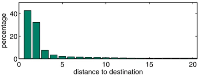
The above observation from Figure 4 is mainly due to the fact that bottlenecks on most of the measured paths are on the last few hops, and different replicas often share bottle-necks. Figure 5 plots the distribution of bottlenecks for the 67,271 destinations of which the last hop can be measured by Pathneck. Thex-axis is the hop distance from bottleneck hop to destination, they-axis is the percentage of destina-tions in each category. We observe that 75% of destinadestina-tions
0 5 10 15 20 0 20 40 distance to destination percentage
Figure 5. Bottleneck location distribution
have bottleneck on the last two hops, and 42.7% on the last hop.
Replicas can improve bandwidth performance if paths from different replicas to a destination have different bot-tlenecks and have different bottleneck bandwidths. Unfor-tunately, we find that in most cases the replicas either share bottlenecks, or have different bottleneck locations but the bottleneck links have very similar bandwidths. This leaves us little opportunity to improve bandwidth performance us-ing replicas for end users. In some cases, we do observe different bottleneck bandwidths from different replicas, but that is because of traffic-load changes instead of bottle-neck location changes. That is, the difference between the “best” curve in Figure 4 and those from individual replicas is mainly due to traffic-load changes.
To filter out the impact of traffic-load changes on band-width distribution, we select a bandband-width measurement for each destination that is most representative among those from all 18 replicas. This is done by splitting the 18 band-width measurements into several groups, and by taking the median value of the largest group as the representa-tive bandwidth. The group is defined as the follows. Let
G be a group, and x be a bandwidth value, x ∈ G iff
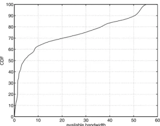
∃y, y ∈ G,|(x−y)/y| < 0.3. Figure 6 plots the dis-tribution of the representative available bandwidths for the 67,271 destinations for which Pathneck can measure the last hop. To the best of our knowledge, this is the first result on the distribution of Internet-scale end-user access band-width. We observe that 40% of destinations have bottleneck bandwidth less than 2.2Mbps, 50% are less than 4.2Mbps, and 63% are less than 10Mbps. These results show that small capacity links still dominate Internet end-user con-nections. In such cases, it is difficult to use replicas to im-prove bandwidth performance because bottlenecks are very likely due to small-capacity last-mile links such as DSL, cable-modem, and dial-up links.
For the destinations with bottleneck bandwidth larger than 10Mbps, the bottleneck bandwidth is almost uniformly distribute in the range of [10Mbps, 50Mbps]2. For these
2The distribution curve in Figure 6 ends at 55.2Mbps. This is a bias
0 10 20 30 40 50 60 0 10 20 30 40 50 60 70 80 90 100 available bandwidth CDF
Figure 6. Distribution of Internet end-user ac-cess bandwidth 0 5 10 15 20 0 5 10 15 20 25 30 35 40 45 50 55 0 0 0 0 0 0 0 0 0 0 0 0 0 0 0 0 0 0 0 0 1 1 1 1 1 1 1 1 1 1 1 1 1 1 1 1 1 1 1 1 2 2 2 2 2 2 2 2 2 2 2 2 2 2 2 2 2 2 2 2 3 3 3 3 3 3 3 3 3 3 3 3 3 3 3 3 3 3 3 3 4 4 4 4 4 4 4 4 4 4 4 4 4 4 4 4 4 4 4 4 5 5 5 5 5 5 5 5 5 5 5 5 5 5 5 5 5 5 5 5 distance to destination percentage
Figure 7. Bottleneck distribution for destina-tions with different available bandwidth
destinations, high-bandwidth bottlenecks are more likely to be determined by link load instead of by link capac-ity, and bottlenecks more frequently appear in the mid-dle of paths. This observation is illustrated in Figure 7, where we split the 67,271 destinations used in Figure 5 into different groups based on bottleneck bandwidth, and plot the distribution of bottleneck locations for each group. The curve marked with “i” represents the group of desti-nations which have bottleneck bandwidth in the range of [i∗10M bps,(i+ 1)∗10M bps). We can see that while groups 0 ∼ 3 have distributions very similar with that
replicas are generally less than 60Mbps, which determines the maximum bottleneck bandwidth that we can detect.
shown in Figure 5, groups 4 and 5 are clearly different. For example, 62% of destinations in group 5 have bottlenecks that are over 4 hops away from the destinations, where dif-ferent replicas have a higher probability of having difdif-ferent routes and thus different bottlenecks. Section 4.3 discusses how to make use of this opportunity to avoid bottlenecks by using different replicas for different destinations.
4
Optimizing RTT and Bandwidth
We have seen that replicas have the potential to improve RTT performance for most destinations, and to improve bandwidth performance for well provisioned destinations. In this section, we present an algorithm that allows us to select replicas to optimize client performance. We then use this algorithm to study how to improve RTT and bandwidth using our measurement infrastructure.
4.1
The Greedy Algorithm
To optimize client performance using replicas, we need to know how many replicas we should use and where they should be deployed. The goal is that the selected set of repli-cas should have performance very close to that achieved by using all replicas. A naive way is to consider all the possible combinations of replicates when selecting the optimal one. Given that there are218−1(i.e., 262,143) different com-binations for 18 replicas, and each replica measures over 160K destinations, the time of evaluating all combinations is prohibitively high. Therefore, we use a greedy algorithm, which is based on a similar idea as the greedy algorithm used in Qiu et.al. [21]. This algorithm only needs polyno-mial processing time, but can find a sub-optimal solution very close to the optimal one. We now explain how to apply this algorithm on the data sets we have.
The intuition behind the greedy algorithm is to always pick the best replica among the available replicas. For ex-ample, in Figure 3,S01is better thanS17andS18for RTT optimization, so S01 should be selected before the other two. In this algorithm, the “best” is quantified using a met-ric calledmarginal utility. In the following, we explain how this metric is computed.
We use RTT optimization as the example. Assume that at some point, some replicas have already been selected. The best RTT from among the selected replica to each destina-tion is given by{rtti|0≤i < N}, whereN ≈160Kis the number of destinations, andrttiis the smallest RTT that is
measured by one of the replicas already selected to desti-nationi. Let{srtti|0 ≤i < N} be the sorted version of
{rtti}. We can now computertt sumas:
rtt sum=
99
k=0
where
index(k) =N×(k+ 1)
101 −1
Intuitively, {srtti|0 ≤ i < N} corresponds to the x -axis values of the points on the CDF curves in Figure 3, andrtt sumcorresponds to the area enclosed by the CDF curve, the lefty-axis, and the topx-axis.
There are two details that need to be explained in the above computation. First, we cannot simply add all the individual measurement when calculatingrtt sum. This is because by definition, a joint node is not necessarily shared by all the measurement sources, so introducing a new replica could bring in measurements to new destina-tions, thus changing the value ofN. Therefore, we cannot simply add allrtti since the data sets would be
incompa-rable. In our analysis, we add 100 values that are evenly distributed on the CDF curve. Here, the number “100” is empirically selected as a reasonably large value to split the curve. Second, we split the curve into 101 segments us-ing 100 splittus-ing points, and only use the values of these 100 splitting points. That is, we do not use the two end values—srtt0 andsrttN−1, whose small/large values are
very probably due to measurement error.
Suppose a new replicaAis added, manyrttican change,
and we compute a newrtt sumA. The marginal utility of
Ais then computed as:
marginal utility=|rtt sum−rtt sumA| rtt sum
With this definition, the replica selected in each step is the one that has the largest marginal utility. For the first step, the replica selected is simply the one that has the smallest
rtt sum. In the end, the algorithm generates areplica se-lection sequence:
v1, v2, ..., v18
wherevi ∈ {S01, S02, ..., S18}. To selectm(<18)
repli-cas, we can simply use the firstmreplicas in this sequence. For bandwidth optimization, the greedy algorithm works in a similar way exceptbwishould be thelargestbandwidth
measured from one of the selected replicas. This greedy algorithm has polynomial processing time, but only gives a sub-optimal solution. In the following section, we will show that the greedy algorithm produces solutions that are very close to optimal.
4.2
RTT Optimization
As demonstrated in Section 3.1, RTT performance is closely related with replica location. In this section, we look at the number of replicas needed to improve RTT.
Figure 8 shows the results of RTT optimization using our greedy algorithm on all valid destinations. The top figure
0 50 100 150 200 250 300 0 0.1 0.2 0.3 0.4 0.5 0.6 0.7 0.8 0.9 1 1 1 1 2 2 2 3 3 3 4 4 4 5 5 5 9 9 9 18 18 18 rtt (ms) % of prefixes 2 4 6 8 10 12 14 16 18 0 0.05 0.1 0.15 0.2 number of sources RTT marginal utility
Figure 8. RTT optimization using greedy algo-rithm.
plots the cumulative distribution of RTT with different num-bers (marked on the curves) of replicas. For clarity, we only plot the results when RTT<300ms, though some RTTs are as large as 3 seconds. The bottom figure plots the marginal utility for each new replica added3. Clearly, the first five
replicas improve the performance most significantly. The marginal utilities from additional replicas are all less than 5%.
In addition, it is interesting to note the different pat-terns of RTT improvement with each of the first five repli-cas added. As we can see from the top figure, adding the second replica improves RTT over a very large range [30ms, 300ms], though the improvement in the range [50ms, 100ms] is the largest. Adding the third replica mainly improves RTT in the ranges [30ms, 100ms] and [150ms, 250ms]; adding the fourth replica improves RTT in the range [70ms, 200ms], but with a slightly lower mag-nitude; and adding the fifth replica improves RTT in the range [10ms, 50ms], with a further reduced magnitude.
Not surprisingly, these differences are mainly due to the different geographic locations of the replicas. As listed in
3This curve starts from the second replica because the first one is
lected using a different method. Also the marginal utility of the third se-lected source is larger than that of the second. This is possible because in the marginal-utility formula thertt sumused to select the third source is less than that used to select the second.
the row labeled “rtt-all” in Table 2—the first five are from US east-coast, Europe, US west-coast, East Asia, and US middle, respectively, which are consistent with common in-tuition. If we consider these geographic locations together with the delay range that is most improved by each replica, we can gain a better understanding of how replicas con-tribute to the performance improvement for destinations in different physical locations.
The greedy algorithm theoretically only provides sub-optimal solutions. To understand how well it approximates the optimal solution, we compare the results in Figure 8 with the best solution obtained using a brute-force search. Obviously, brute-force search can not explore all the possi-ble combinations of the 18 replicas, as explained before. However, we have seen that the first five replicas domi-nate performance gains. Given the computing resources we have, we can go through all possible four-replica combi-nations in five hours. Therefore, we compute thertt sum
values for all four-replica combinations, and select the best one to compare with the first four replicas selected by our greedy algorithm. Using this method, we find that the so-lution obtained using our greedy algorithm for RTT opti-mization is the 7th best among all of the 3,060 four-replica combinations, and it is only 0.1% worse than the best so-lution (S04S14S16S18). Such small difference shows that the greedy algorithm indeed finds a solution close to the optimal one.
4.3
Bandwidth Optimization
Section 3.2 shows that replicas have higher probability to improve bandwidth performance for well provisioned des-tinations, since they have higher probability to experience different bottlenecks for such destinations. In this section, we use the greedy algorithm to study how to make use of this opportunity. We look at two cases. In the first case, we only use the 23,447 destinations where Pathneck can mea-sure the last hop, and the bottleneck bandwidth is higher than 40Mbps. In the second case, we include all valid des-tinations.
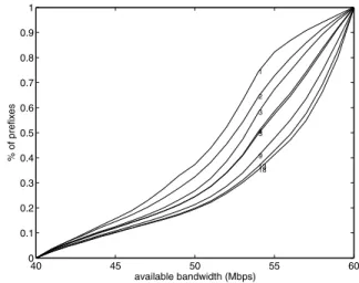
The results of the first case study are shown in Fig-ure 9. It shows the cumulative distribution of path band-width upper-bounds with varying numbers of replicas. We can see that the bandwidth improvement from replicas is indeed significant. For example, with a single replica, there are only 26% paths that have bandwidth higher than 54Mbps, while with all 18 replicas, the percentage increases to 65%.
An obvious problem for the first case study is that it only covers around 16% of the paths that we measured, thus the results could be biased. To do a more general study, we apply the greedy algorithm on all the valid destinations, but exclude last-mile bottlenecks. In other words, we do
40 45 50 55 60 0 0.1 0.2 0.3 0.4 0.5 0.6 0.7 0.8 0.9 1 1 2 3 4 5 9 13 18 available bandwidth (Mbps) % of prefixes
Figure 9. Bandwidth optimization for well pro-visioned destinations. 0 10 20 30 40 50 60 0 0.1 0.2 0.3 0.4 0.5 0.6 0.7 0.8 0.9 1 1 1 2 2 3 3 4 4 5 5 9 9 13 13 18 18 available bandwidth (Mbps) % of prefixes 2 4 6 8 10 12 14 16 18 0 0.02 0.04 0.06 0.08 0.1 number of sources
bandwidth marginal utility
Figure 10. Bandwidth optimization for all valid destinations.
a “what if” experiment to study what would happen if last-mile links were upgraded. That is, for those destinations where Pathneck can measure the last hop, we remove the last two hops; this is based on the observation in Figure 5 that 75% paths have bottlenecks on the last two hops. For the others, we use the raw measurement results. Figure 10
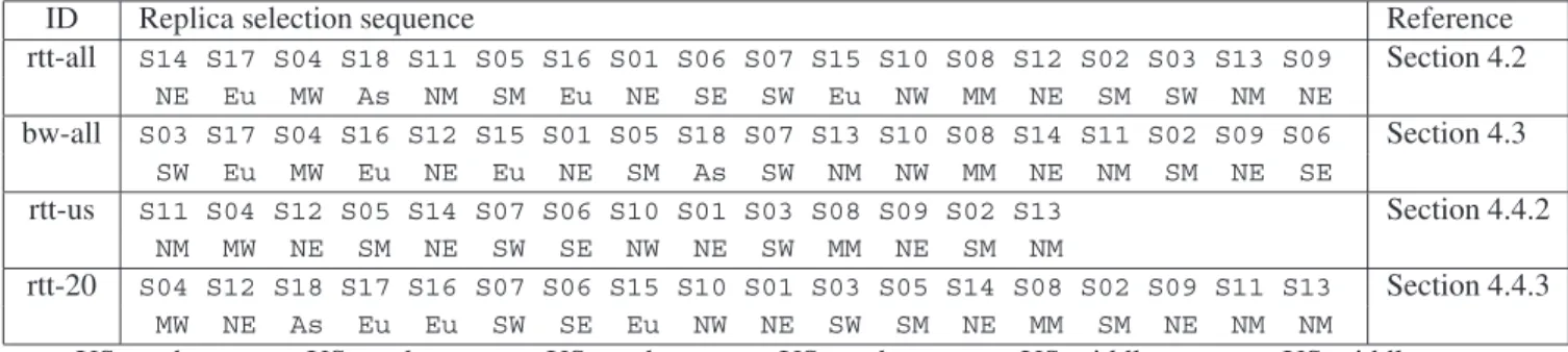
Table 2. The replica selection sequence (with location code) determined by the greedy algorithm
ID Replica selection sequence Reference
rtt-all S14 S17 S04 S18 S11 S05 S16 S01 S06 S07 S15 S10 S08 S12 S02 S03 S13 S09 Section 4.2 NE Eu MW As NM SM Eu NE SE SW Eu NW MM NE SM SW NM NE bw-all S03 S17 S04 S16 S12 S15 S01 S05 S18 S07 S13 S10 S08 S14 S11 S02 S09 S06 Section 4.3 SW Eu MW Eu NE Eu NE SM As SW NM NW MM NE NM SM NE SE rtt-us S11 S04 S12 S05 S14 S07 S06 S10 S01 S03 S08 S09 S02 S13 Section 4.4.2 NM MW NE SM NE SW SE NW NE SW MM NE SM NM rtt-20 S04 S12 S18 S17 S16 S07 S06 S15 S10 S01 S03 S05 S14 S08 S02 S09 S11 S13 Section 4.4.3 MW NE As Eu Eu SW SE Eu NW NE SW SM NE MM SM NE NM NM
NE: US northeast,NW: US northwest,SE: US southeast,SW: US southwest,ME: US middle-east,MW: US middle-west
MM: US middle-middle,Eu: Europe,As: Asia
includes the results from the greedy algorithm when consid-ering all destinations. The row “bw-all” in Table 2 lists the replica selection sequence from the greedy algorithm, and the marginal utility from each replica. We can see that the bandwidth improvement spreads almost uniformly in the large range [5Mbps, 50Mbps]. If using 5% as the thresh-old for marginal utility, only the first two replicas selected significantly contribute to the bandwidth performance im-provement. From the row “bw-all” in Table 2, we note that geographic diversity does not play an important role. All these observations are very different from the results for RTT optimization.
4.4
Variants of RTT Optimization
In this section, we briefly present the results from three variants of the RTT optimization problem discussed in Sec-tion 4.2.
4.4.1 Weighting Destinations Using Web Server Load
So far we have assumed that clients from different prefixes have equal probability to request service, but this is not the case for many Internet services. To consider non-uniform client distributions, we obtained client request logs from five popular Web sites in the US to weight the RTT measure-ments. That is, the raw RTT to each destination is weighted using the total amount of packets exchanged with the clients that share the same prefix with the destination in our mea-surements.
The statistics of these Web logs are listed in columns 2-4 in Table 3. We can see that the client population only covers 5∼10% of the prefixes that we measured. To weight the RTT measurements, we first compute the number of packets sent from a Web site to each of its clients. We then cluster these clients based on their network prefixes, obtain the total number of packets exchanged with each prefix (denoted as
pktifor prefixi). If the RTT to prefixiis measured asrtti,
we use(rtti×pkti)as the input to the greedy algorithm. We
do not consider those prefixes which do not have any clients in the Web logs. Bandwidth measurements are weighted in similar way.
Applying the greedy algorithm on the weighted RTT val-ues shows that the first five replicas still dominate the RTT performance improvement. However, the replica selection sequences, as listed in the last column of Table 3, are very different from those obtained when giving all prefixes equal weight. First, the replicas outside the US are less important. Second, for all five Web sites, the first four replicas are al-ways from NE, NM, SM, SW/MW, i.e., evenly distributed in the US. This clearly indicates that the client distributions of these Web sites are biased toward US users.
4.4.2 US Replicas Only
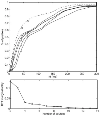
To consider the scenarios where deploying a replica out-side the US is hard, we look at the case where we only use the 14 replicas inside the US. Using the same method as that in Section 4.2, we obtain the results as shown in Fig-ure 11 and the “rtt-us” row in Table 2. The dashed curve in the top graph of Figure 11 is the RTT performance when using all 18 replicas; it is copied from Figure 8 for com-parison. We can see that only 55% of paths have RTT less than 50ms when using the US-only replicas, which is 13% worse than that when using all 18 replicas. Second, compar-ing with the brute-force solutions obtained in Section 4.2, the performance from the first four replicas selected here is 25% worse than the greedy-algorithm solution when using all replicas. These two results quantify the importance of replicas in Europe and East-Asia for RTT optimization. Fi-nally, with the US-only replicas, only the first three replicas have marginal utilities larger than 5%, and they are from the middle, the east coast, and the west coast of the US, which again highlights the importance of diverse geographic
loca-Table 3. Replica selection sequence weighted by Web server load (measured in 47 hours)
Number of Load Load
prefixes (byte) (pkt) RTT Web1 9759 235G 369M S14 S05 S07 S11 S06 S17 S04 S01 S12 S10 S03 S08 S15 S09 S18 S02 S16 S13 Web2 16412 163G 337M S14 S07 S11 S05 S15 S04 S18 S06 S01 S10 S16 S08 S12 S03 S09 S17 S02 S13 Web3 16244 157G 182M S11 S14 S04 S05 S01 S07 S06 S17 S10 S08 S02 S18 S12 S09 S16 S13 S03 S15 Web4 8113 23G 203M S14 S05 S04 S11 S06 S17 S07 S01 S08 S12 S10 S16 S02 S13 S18 S09 S03 S15 Web5 17484 124G 157M S14 S07 S11 S05 S17 S06 S04 S12 S18 S10 S01 S15 S08 S16 S03 S02 S09 S13 0 50 100 150 200 250 300 0 0.1 0.2 0.3 0.4 0.5 0.6 0.7 0.8 0.9 1 1 1 1 2 2 2 3 3 3 4 4 4 14 14 14 18 18 18 rtt (ms) % of prefixes 2 4 6 8 10 12 14 0 0.05 0.1 number of sources RTT marginal utility
Figure 11. RTT optimization using only repli-cas in the US.
tions for RTT optimization.
4.4.3 Optimizing The Worst Performance
A previous study [12] has pointed out that CDNs can im-prove performance by simply avoiding directing clients to the worst replica. Based on this observations, we look at how well the infrastructure works if we focusing on im-proving the clients that have the worst performance. Specif-ically, we computertt sum in such a way that only the worst 20% of the destinations are included, and then select the replica that can optimize this metric. The “rtt-20” row in Table 2 lists the replica selection sequences. The main difference with the results that consider all destinations is
that there is one more European node in the top five repli-cas. Compared with the brute-force solution obtained in Section 4.2, the performance of the first four replicas is only 1.3% worse than that of the optimal four-replica set. Over-all, we did not see a major improvement compared with the case where all destinations are considered.
5
Performance of Applications
The analysis in the previous section has shown that repli-cas can significantly improve RTT performance, but have much less impact on bandwidth performance due to bottle-neck sharing. However, the performance of network appli-cations is determined by data transmission time, which de-pends not only on RTT and available bandwidth, but also on data size. In this section, we consider these three factors to study the benefit of using replicas to reduce data transmis-sion time. Below we first provide a simplified TCP model to characterize data transmission time as a function of avail-able bandwidth, RTT, and data size. We then look at the transmission-time distribution for different data sizes with different number of replicas.
5.1
Simplified TCP Throughput Model
Simply speaking, TCP data transmission includes two phases: slow-start and congestion avoidance [9]. During slow-start, the sending rate doubles every roundtrip time, because the congestion window exponentially increases. During congestion avoidance, the sending rate and the con-gestion window only increase linearly. These two algo-rithms, together with the packet loss rate, can be used to de-rive an accurate TCP throughput model [20]. However, we can not use this model since we do not know the packet loss rate, which is very expensive to measure. Instead, we build a simplified TCP throughput model that only uses band-width and RTT information.
Our TCP throughput model is as follows. Let the path under considered have available bandwidthabw(Bps) and roundtrip timertt(second). Assume that the sender’s TCP
congestion window starts from 2 packets and that each packet is 1,500 bytes. The congestion window doubles ev-ery RTT until it is about to exceed the bandwidth-delay product of the path. After that, the sender sends data at a constant rate of abw. This transmission algorithm is sketched in the code segment shown below. It computes the total transmission time (ttotal) forxbytes of data along
a path.
cwin = 2 * 1500; t_ss = 0; t_ca = 0;
while (x > cwin && cwin < abw * rtt) { x -= cwin; cwin *= 2; t_ss += rtt; } if (x > 0) t_ca = x / abw; t_total = t_ss + t_ca;
wheret ssandt caare the transmission time spent in the slow-start phase and the congestion avoidance phase, re-spectively. We say the data transmission isrtt-determinedif
t ca= 0. We can easily derive the maximum rtt-determined data size as
2log2(abw∗rtt/1500)+1∗1500(
byte)
In the following, we call this size the slow-start size. Clearly, when the data is less than the slow-start size, it is rtt-determined.
This model ignores many important parameters that can affect TCP throughput, including packet loss rate and TCP timeout. However, the purpose of this analysis is not to compute an exact number, but rather to provide a guideline on the range of data sizes where RTT should be used as the optimization metric in replica hosting.
5.2
Slow-Start Sizes and Transmission Times
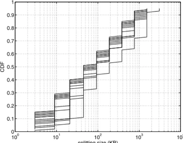
Using the above model, we compute the slow-start sizes for the 67,271 destinations for which Pathneck can obtain complete measurements. Figure 12 plots the distributions of slow-start sizes for the paths starting from each replica. Different replicas have fairly different performance; differ-ences are as large as 30%. Overall, at least 70% of paths have slow-start sizes larger than 10KB, 40% larger than 100KB, and around 10% larger 1MB. Given that web pages are generally less than 10KB, it is clear that their transmis-sion performance is dominant by RTT and replica place-ment should minimize RTT. For data sizes larger than 1MB, replica deployment should focus on improving bandwidth.To obtain concrete transmission times for different data sizes, we use our TCP throughput model to compute data transmission time on each path for four data sizes: 10KB,
100 101 102 103 104 0 0.1 0.2 0.3 0.4 0.5 0.6 0.7 0.8 0.9 1 splitting size (KB) CDF
Figure 12. Cumulative distribution of the slow-start sizes 0 0.5 1 1.5 2 0 0.2 0.4 0.6 0.8 1 1 1 1 2 2 2 5 5 5 9 9 9 18 18 18 % of prefixes
xfer time (s) for 10KB
0 1 2 3 4 5 0 0.2 0.4 0.6 0.8 1 1 1 1 2 2 2 5 5 5 9 9 9 18 18 18 % of prefixes
xfer time (s) for 100KB
0 10 20 30 40 0 0.2 0.4 0.6 0.8 1 1 1 1 2 2 2 5 5 5 9 9 9 18 18 18 % of prefixes
xfer time (s) for 1MB
0 100 200 300 0 0.2 0.4 0.6 0.8 1 1 1 1 2 2 2 5 5 5 9 9 9 18 18 18 % of prefixes
xfer time (s) for 10MB
Figure 13. Transmission times for different data sizes
100KB, 1MB, and 10MB. We then use the greedy algorithm to optimize data transmission times. The four subgraphs in Figure 13 illustrate the transmission-time distributions for each data size using different number of replicas. These figures are plotted the same way as that used in Figure 8. If we focus on the 80 percentile values when all 18 replicas are used, we can see the transmission times for 10KB, 100KB, 1MB and 10MB are 0.4 second, 1.1 second, 6.4 second, and 59.2 second, respectively. These results are very useful for Internet-scale network applications to obtain an intuitive
understanding about their data transmission performance.
6
Related Work
Content replication has been widely applied in real net-work systems [1, 2]. The replication could be done for the whole mirror/proxy server, or for selected content objects. CDNs [22] generally belong to the former, while peer-to-peer systems [25, 29] belong to the later. Our work is dis-cussed in the context of server replication, but the results presented in this paper can also be applied for object repli-cation.
The key question in content replication is how to deploy the replicas, including where to replicate and how many replicas should be used. Multiple solutions have been de-veloped and two good overviews on these solutions can be found in [24, 14]. Different solutions often have differ-ent optimization goals, which include geographic location [19], network hops and latency [6, 23, 4, 18], retrieval costs [17, 16], update cost [27, 11], storage cost [5, 15], and QoS guarantee [26]. Many of the previous work considered two or three metrics together. For example, [27, 11] considered update cost and retrieval cost, [5, 15] considered storage cost and retrieval cost, while [13] considered three metrics: retrieval, update, and storage cost. More recently, [28] looks at the opportunities of optimizing a hosting service by deal-ing with network failures. To the best of our knowledge, no related work has studied the problem of optimizing bot-tleneck bandwidth performance. In addition, though prop-agation delay and transmission time have been considered by previous work, few of them considered these metrics in Internet-scale deployments. These are the two main differ-ences between our work and the previous work, and they are also the main contributions of this paper.
In our work, we show that the performance gain becomes minimal after a number of replicas have been deployed. This is consistent with the observation in [10]. Our work is distinguished from [10] in the sense that we also study the geographic factor on replica placement and provide guid-ance based on the size of content objects.
Independent of the metrics used to optimize content dis-tribution, greedy algorithms can often provide good solu-tions. The greedy algorithm proposed in our paper has near optimal solution. This is also consistent with the conclusion in [21], which compared several heuristics and found that a simple greedy algorithm works best. Greedy algorithms are also used in [26], which developed both “Greedy-Insert” and “Greedy-Delete” algorithms to solve QoS-aware place-ment problems.
7
Conclusion
In this paper, we use a set of large scale Internet measure-ments from 18 geographically diverse measurement sources to study how to optimize RTT and bandwidth performance in a content replication system. This set of measurements reveal for the first time the distribution of end-user access bandwidth. Based on a greedy algorithm, we show that only five carefully selected replicas are needed to optimize RTT performance in our infrastructure, while only two replicas are needed to optimize bandwidth performance. Moreover, the replicas selected for RTT optimization have a very clear geographic distribution, which is not the case for bandwidth optimization. Using real Web site logs, we also investigate the impact of Web client distribution on RTT performance optimization. We observe that the results are significantly different from those without considering such factor. Fur-thermore, we use a simplified TCP model to show that when the dominant data size of a network service is less than 10KB, replica deployment should optimize RTT; when the dominant data size is larger than 1MB, replica deployment should optimize bandwidth.
Acknowledgments
Ningning Hu and Peter Steenkiste were in part supported by the NSF under award number CCR-0205266.
References
[1] Akamai. http://www.akamai.com.
[2] Digital Island. http://www.digitalisland.com.
[3] The Internet health report. http://www1.internetpulse.net. [4] R. Carter and M. Crovella. Dynamic server selection using
bandwidth probing in wide-area networks. InProc. IEEE INFOCOM, 1997.
[5] I. Cidon, S. Kutten, and R. Soffer. Optimal allocation of electronic content. InProc. IEEE INFOCOM, April 2001. [6] S. G. Dykes, K. A. Robbins, and C. L. Jeffery. An
empiri-cal evaluation of client-side server selection algorithms. In Proc. IEEE INFOCOM, 2000.
[7] P. Francis, S. Jamin, C. Jin, Y. Jin, D. Raz, Y. Shavitt, and L. Zhang. Idmaps: A global Internet host distance estima-tion service.IEEE/ACM Transactions on Networking, Octo-ber 2001.
[8] N. Hu, L. Li, Z. Mao, P. Steenkiste, and J. Wang. Locating Internet bottlenecks: Algorithms, measurements, and impli-cations. InProc. ACM SIGCOMM, August 2004.
[9] V. Jacobson. Congestion avoidance and control. InProc. ACM SIGCOMM, August 1988.
[10] S. Jamin, C. Jin, A. R. Kurc, D. Raz, and Y. Shavitt. Con-strained mirror placement on the internet. InProc. IEEE INFOCOM, April 2001.
[11] X. Jia, D. Li, X. Hu, W. Wu, and D. Du. Placement of web-server proxies with consideration of read and update oper-ations on the internet. The Computer Journal, 46(4), July 2003.
[12] K. Johnson, J. Carr, M. Day, and M. Kaashoek. The mea-sured performance of content distribution networks. InProc. of the 5th International Web Caching and Content Delivery Workshop, May 2000.
[13] K. Kalpakis, K. Dasgupta, and O. Wolfson. Optimal place-ment of replicas in trees with read, write, and storage costs. IEEE Transactions on Parallel and Distributed Systems, 12(6):628–637, June 2001.
[14] M. Karlsson, M. Mahalingam, and C. Karamanolis. A framework for evaluating replica placement algorithms. Technical Report HPL-2002-219, HP Laboratories. [15] M. R. Korupolu and M. Dahlin. Coordinated placement and
replacement for large-scale distributed caches. IEEE Trans-actions on Knowledge and Data Engineering, 14(6):1317– 1329, 2002.
[16] P. Krishnan, D. Raz, and Y. Shavitt. The cache location prob-lem. IEEE/ACM Transactions on Networking, 8(5):568– 582, October 2000.
[17] B. Li, M. J. Golin, G. F. Italiano, X. Deng, and K. Sohraby. On the optimal placement of web proxies in the internet. In Proc. IEEE INFOCOM, April 1999.
[18] P. McManus. A passive system for server selection within mirrored resource environments using AS path length heuristics. http://pat.appliedtheory.com/bgpprox/.
[19] NetGeo – the Internet Geographic Database.
http://www.caida.org/Tools/NetGeo/. [20] J. Padhye, V. Firoiu, D. Towsley, and J. Kurose. Modeling
TCP throughput: A simple model and its empirical valida-tion. InProc. ACM SIGCOMM, September 1998.
[21] L. Qiu, V. N. Padmanabhan, and G. M. Voelker. On the placement of web server replicas. InProc. IEEE INFOCOM, April 2001.
[22] M. Rabinovich and O. Spatscheck.Web Caching and Repli-cation. Addison-Wesley, 2002.
[23] M. Sayal, Y. Breitbart, P. Scheuermann, and R. Vingralek. Selection algorithms for replicated web servers. InProc. of the Workshop on Internet Server Performance, June 1998. [24] S. Sivasubramanian, M. Szymaniak, G. Pierre, and M. van
Steen. Replication for web hosting systems. ACM Comput. Surv., 36(3):291–334, 2004.
[25] I. Stoica, R. Morris, D. Karger, M. Kaashoek, and H. Bal-akrishnan. Chord: A scalable peer-to-peer lookup service for internet applications. InProc. ACM SIGCOMM, August 2001.
[26] X. Tang and J. Xu. On replica placement for qos-aware con-tent distribution. InProc. IEEE INFOCOM, April 2004. [27] J. Xu, B. Li, and D. L. Lee. Placement problems for
transparent data replication proxy services. IEEE Journal on Selected Areas in Communications, 20(7):1383–1398, September 2002.
[28] M. Zhang, C. Zhang, V. Pai, L. Peterson, and R. Wang. Plan-etseer: Internet path failure monitoring and characterization in wide-area services. InProc. OSDI, December 2004. [29] B. Zhao, J. Kubiatowicz, and A. Joseph. Tapestry: An
in-frastructure for fault-tolerant wide-area location and routing. Technical Report UCB/CSD-01-1141, UCB.