Radar Backscatter Modeling Based on
Global TanDEM-X Mission Data
Zur Erlangung des akademischen Grades einer
DOKTOR-INGENIEURIN
von der Fakultät für
Elektrotechnik und Informationstechnik der Universität Fridericiana Karlsruhe (TH)
genehmigte
DISSERTATION
von
M.Sc. Paola Rizzoli
geb. in Sarnico, Bergamo, Italien
Tag der mündlichen Prüfung: 05. 10. 2018
Hauptreferent: Prof. Dr.-Ing. habil. Alberto Moreira
È dunque sognando ad occhi aperti, io credo, che vivi intensamente; ed è ancora con l’immaginazione che puoi trovarti a competere persino con l’inattuabile. E qualche volta ne esci anche vincitore. Walter Bonatti
Acknowledgements
I would like to thank Prof. Dr. Alberto Moreira, director of the DLR Microwaves and Radar Institute, for his constant guidance throughout the development of this work. Thank you to my supervisors, Dr. Manfred Zink and Dr. Benjamin Bräutigam, for their great support and for constantly motivating me to conclude the PhD. My gratitude goes to Prof. Dr. Helmut Rott for his highly valuable technical support and for accepting to be the co-reviewer of this thesis.
I also would like to thank all the other members of my research group for their support, the interesting discussions, and their availability to review the manuscript: Michele Mar-tone, Christopher Wecklich, Carolina Gonzalez, Andrea Pulella, José-Luis Bueso-Bello, Paolo Valdo, and Nicola Gollin.
I thank all the colleagues at DLR who helped me to improve the quality of the thesis and of the final presentation and to organize all the formalities for the PhD defense at the University of Karlsruhe. In particular, I am grateful to Dr. Daniela Borla Tridon, Dr. Francescopaolo Sica, Dr. Matteo Nannini, Dr. Michelangelo Villano, Dr. Claudio Castellini, Dr. Muriel Pinheiro, Dr. Felipe Queiroz de Almeida, Dr. Sigurd Huber, Dr. Giuseppe Parrella, and Dr. to be Georg Fischer.
Moreover, a sincere acknowledgement goes to all other colleagues at DLR and to all my friends in Munich for their company in the everyday life. I specially thank my German connection and dearest friends Uli and Alex, for the great time together and for unlocking the secrets of the German (and Bavarian) society. Thank you also to Elisa and Michele for their long-lasting friendship, that I allow myself to call brotherhood. And thank you to Nadia, for taking me with her to the top of the mountains and showing me the world from other perspectives.
I am deeply grateful to my parents, my sister, and Indy for always loving and supporting me and sharing good and bad times together.
Finally, I would like to dedicate this work to the memory of my grandmother Peppina, whose unconditioned love will accompany me for the rest of my life.
Radarrückstreuung bezeichnet den Teil eines ausgesendeten elektromagnetischen Sig-nals, der von einem Ziel am Boden wieder zurück zur Antenne gerichtet ist. Die Eigen-schaften des zurückgestreuten Signals ändern sich in Abhängigkeit von Frequenz und Polarisation des Radarsignals, der Aufnahmegeometrie, sowie vom Zustand des Erdbo-dens und der Art der Bodenbedeckung. Informationen über das Radarrückstreuverhal-ten sind von höchster Wichtigkeit für die Auslegung von SAR-Missionen und werden verbreitet zur Entwicklung wissenschaftlicher Modelle genutzt, beispielsweise bei der Erforschung der Biosphäre und Kryosphäre. Hauptziel dieser Arbeit ist die Auswertung und Nutzung des globalen TanDEM-X-Datensatzes zur Modellierung der Radarrück-streuung im X-Band unter Berücksichtigung unterschiedlicher Aufnahmeparameter und Landnutzungsarten, sowie die Bereitstellung einer Reihe von globalen Rückstreumod-ellen, die auf aktuellen Daten basieren, für die wissenschaftliche Gemeinschaft. Es wurde ein neuer Ansatz zur statistischen Modellierung der Rückstreuinformation en-twickelt, der die Qualität der zugrunde liegenden Messungen berücksichtigt. Daraus ergeben sich gewichtete polynomiale Modelle für die verschiedenen Landnutzungsarten,
wie sie in derGlobCover-Karte der ESA definiert sind. Darüber hinaus wird ein eigener
Validierungsansatz vorgestellt, mit zusätzlicher Betrachtung der saisonalen Variation der Rückstreuung und einer separaten Analyse des Rückstreuverhaltens des Tropischen Re-genwaldes. Der nächste Schwerpunkt ist die Betrachtung des Grönländischen Eiss-childes, das gekennzeichnet ist durch das Vorhandensein verschiedener Arten von Schnee-bedeckung, die von trockenem bis hin zu sehr feuchtem Schnee variiert. Der
begren-zte Detailgrad, den die GlobCover Karte in Grönland aufweist (nur eine Klasse für
das gesamte Eisschild), erlaubt dort keine verlässliche Modellierung der Rückstreuung. Diese Schwierigkeit lieferte die Motivation für die Entwicklung eines neuen Ansatzes zur Analyse des Informationsgehalts der interferometrischen TanDEM-X-Daten mit dem Ziel, unterschiedliche Schnee-Fazien mit Hilfe des sog. C-Means Fuzzy Clustering Algorithmus zu lokalisieren. Aus dieser Untersuchung konnte die Existenz von vier unterschiedlichen Klassen von Schnee-Fazien abgeleitet werden, deren Eigenschaften anschließend mit Hilfe externer Referenzdaten interpretiert wurden. Die daraus ent-standene Karte wurde zur Erstellung eines einfallswinkelabhängigen Rückstreumodells genutzt, separat für jede der vier Klassen, wobei eine modifizierte Version des entwickel-ten Algorithmus zur Generierung globaler Rückstreumodelle eingesetzt wurde. Darüber hinaus wurde als Nebenprodukt zusätzlich die Eindringtiefe von TanDEM-X in die Eiss-chicht geschätzt, durch Inversion des von Weber Hoen und Zebker vorgeschlagenen "Ein-chicht-Volumendekorrelationsmodells". Die Ergebnisse wurden mit dem
Höhe-nunterschied zwischen dem globalen TanDEM-X-DEM und ICESat-Messungen ver-glichen. Abschließend wird ein neu entwickelter Algorithmus zur Generierung von Rückstreukarten großer Gebiete vorgestellt. Dieser erlaubt unter Verwendung von Rück-streumodellen das Angleichen der erstellten Karten anhand eines Referenzeinfallswin-kels, was dann das Füllen verbleibender Lücken ermöglicht, die aufgrund fehlender Ein-gangsdaten vorhanden sind.
Radar backscatter represents the portion of a transmitted electromagnetic signal that is redirected back toward the antenna from a target on ground. Its properties change de-pending on the radar wave frequency and polarization, acquisition geometry, ground cover type, and soil conditions. Backscatter information is of paramount importance for the design of SAR missions and is widely used for the development of scientific models in the fields of, e.g., the biosphere and cryosphere.
The main goal of this work is to exploit the global TanDEM-X SAR data set to model radar backscatter at X band, considering different acquisition parameters and land cover types and to provide then the scientific community with an up-to-date set of backscatter models at a global scale.
A novel approach for statistically model the backscatter information, which takes into account the quality of the input measurements, has been developed. The results are
weighted polynomial models for different land cover types, taken from the ESA
Glob-Cover map. A dedicated validation approach is presented as well, together with addi-tional considerations on backscatter seasonality and a dedicated analysis of backscatter behavior over tropical rainforests.
The attention is then focused on the Greenland Ice Sheet, which is characterized by the presence of different kinds of snow cover, from dry to wet snow. Here, the insufficient
level of detail that is provided by theGlobCovermap over Greenland (one single class for
the entire ice cap) does not allow for a reliable modeling of backscatter. This obstacle set the motivation for developing a new approach for analyzing the information content of interferometric TanDEM-X data, aimed at locating different snow facies by means of the
c-means fuzzy clustering algorithm. A set of four different snow facies has been derived,
and their properties interpreted with the help of external reference data. The obtained map has then been used to generate an incidence angle dependent backscatter model for each snow facies, separately, by using a modified version of the developed algorithm for the generation of global backscatter models. Moreover, as by-product, the penetration depth of TanDEM-X into the ice pack has been estimated as well, by inverting the volume decorrelation single-layer model proposed by Weber Hoen and Zebker. The results have then been compared to the difference in height between the global TanDEM-X DEM and ICESat measurements.
Finally, an algorithm for the generation of large-scale backscatter maps has been devel-oped as well. It requires the use of backscatter models to equalize the output maps to a certain incidence angle of reference and to eventually fill remaining gaps caused by missing input data.
List of Symbols xi
List of Mathematical Operators xvii
List of Acronyms xviii
1. Introduction 1
1.1. Radar in Remote Sensing . . . 1
1.2. A Historical Overview of Spaceborne SAR . . . 3
1.3. Motivation of the Work . . . 5
1.4. Thesis Structure . . . 6
1.5. Original Contribution of the Thesis . . . 7
2. Theoretical Background 9 2.1. Electromagnetic Waves . . . 9
2.1.1. Electromagnetic Plane Waves . . . 9
2.1.2. Electromagnetic Power Density . . . 13
2.1.3. Wave Polarization . . . 13
2.1.4. Wave Reflection and Transmission at the Interface . . . 14
2.2. Radar Backscattering . . . 16
2.2.1. Scattering Matrix . . . 16
2.2.2. Scattering from a Point Target . . . 17
2.2.3. Scattering from a Distributed Target . . . 18
2.2.4. Surface and Volume Scattering . . . 20
2.2.5. Chapter Remarks . . . 21
3. Principles of SAR Imaging and Interferometry 22 3.1. SAR Image Formation . . . 22
3.1.1. Acquisition Geometry and Resolution . . . 22
3.1.2. Perspective Deformations . . . 26
3.1.3. Range Focusing . . . 26
3.1.4. Azimuth Focusing . . . 27
3.1.5. Image Speckle and Multilooking . . . 28
3.1.6. SAR Acquisition Modes . . . 30
Contents
3.1.8. SAR Image Geocoding . . . 32
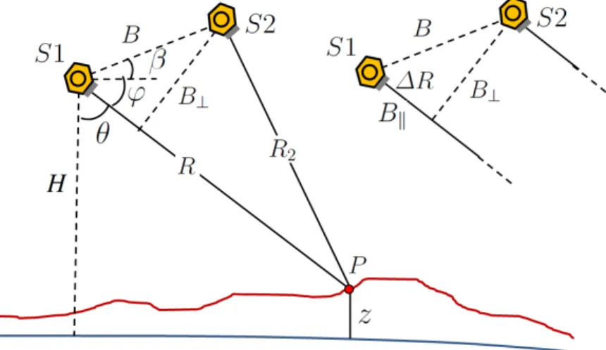
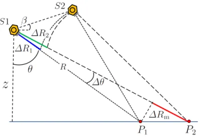
3.2. SAR Interferometry . . . 34
3.2.1. From the Acquisition Geometry to the Height Retrieval . . . 34
3.2.2. The Interferogram . . . 36
3.2.3. Spectral Shift . . . 39
3.2.4. The interferometric Coherence . . . 40
3.2.5. Phase Unwrapping and DEM Generation . . . 40
3.2.6. Chapter Remarks . . . 43
4. The TanDEM-X Mission and its Global Data Set 44 4.1. TerraSAR-X and TanDEM-X Satellites . . . 44
4.2. Mission Overview . . . 45
4.3. TanDEM-X Data: Quicklook Images . . . 50
5. A New Approach for Statistical Modeling of Radar Backscatter 56 5.1. State of the Art in Radar Backscatter Modeling . . . 56
5.2. Mapping Radar Backscatter . . . 57
5.3. A New Method for Modeling Backscatter . . . 58
5.3.1. Backscatter Characterization from Single SAR Acquisitions . . 58
5.3.2. Modeling Algorithm . . . 65
5.3.3. Summary of methods output . . . 69
5.3.4. Discussion upon the Sources of Error . . . 71
5.4. Performance Evaluation Approach of Global Backscatter Models . . . . 75
5.4.1. Check for Absolute Offsets . . . 75
5.4.2. Curvature and Slope Accuracy . . . 77
5.4.3. Combination of Different Test Sites . . . 79
5.5. Seasonal and Geographic Backscatter Dependency . . . 83
5.6. A Large-Scale Study of Tropical Rainforests Backscatter . . . 86
5.6.1. Input Test Sites andγ0Quicklook Mosaics . . . 87
5.6.2. Analysis ofγ0 Incidence Angle Dependency . . . 87
5.6.3. Analysis ofγ0 Seasonal Dependency . . . . 90
6. The Greenland Ice Sheet Case 94 6.1. The Greenland Ice Sheet: an Introduction to the Work . . . 95
6.2. Fuzzy Clustering for Snow Facies Classification . . . 97
6.2.1. Thec-Means Fuzzy Clustering Optimization . . . 98
6.2.2. Algorithm Initialization . . . 99
6.3. Input Data: TanDEM-X Mosaics over Greenland . . . 100
6.3.1. TanDEM-X Input Mosaics . . . 100
6.3.2. Generation of the Ice Sheet Mask . . . 102
6.5. Snow Facies Interpretation and Further Considerations . . . 108
6.5.1. Reference Snow Melt Data . . . 108
6.5.2. In Situ Measurements along the EGIG Line . . . 110
6.5.3. Refined Classification of the Inner Snow Facies . . . 112
6.5.4. Statistical Analysis of the Derived Snow Facies . . . 113
6.5.5. Volume Decorrelation Dependency on the Height of Ambiguity 114 6.6. Applications . . . 115
6.6.1. Backscatter Modeling using Modified Weighting . . . 116
6.6.2. Estimation of the Penetration Depth . . . 120
7. Generation of Backscatter Maps 127 7.1. Generation of Backscatter Mosaics . . . 127
7.2. Global Backscatter Map Final Structure . . . 134
7.3. Filling of Missing Values . . . 135
8. Conclusions and Future Work 138
Bibliography 143
Appendices 158
List of Symbols
a radar brightness quality weight
A reference integration area
Aβ backscatter normalization area in slant range direction
Aγ backscatter normalization area perpendicular to the slant range direction
Aσ backscatter normalization area projected on ground
α local slope B baseline B⊥ normal baseline Bk parallel baseline B⊥,c critical baseline Brg pulse bandwidth
β baseline orientation angle with respect to the local horizontal
β0 radar brightness
β0
unW mean radar brightness unweighted model
β0
W mean radar brightness weighted model
β0
sim simulated radar brightness image
c number of output clusters
C noise covariance matrix for unweighted radar brightness measurements
Cw noise covariance matrix for weighted radar brightness measurements
D DEM in spatial distances coordinates
d(τ) complex chirp in range
daz azimuth pulse repetition time
d1w one-way penetration depth
d2w two-way penetration depth
δβ0 radar brightness correction factor
∆fR spectral shift
∆h mean height difference between ICESat and TanDEM-X
∆H difference between the mean estimated two-way penetration depth and the
∆R range difference
∆θ incidence angle difference
e Euler’s number
regularization term
ε complex dielectric constant
ε0 permittivity of free space
ε0 permittivity of the material relative to that of free space
E electric field intensity
E[·] mean value
E(x, y, z) vector phasor of the electric field
E(x, y, z;t) instantaneous electric field at timet
Ex, Ey, Ez Cartesian components of the electric field phasor
η intrinsic impedance
f frequency
F vector of observations belonging to a single snow facies
¯
Fw mean value of all pixels within the considered boxcar window
fD(taz) Doppler frequency
φ(taz) azimuth phase
φa squint angle
φobj target’s phase within a SAR image
φint interferometric phase
φf e flat Earth phase
φtopo topographic phase
φunw unwrapped phase
ϕ angle between the horizontal and the slant range direction
G fitting Gaussian function
Gt transmitting antenna gain
Gr receiving antenna gain
γ propagation constant
γ0 backscattering coefficient per unit area perpendicular to the antenna beam
γ0
W meanγ0weighted model
γTot total interferometric coherence
γSNR correlation factor due to limited SNR
List of Symbols
γAmb correlation factor due to ambiguities
γRg correlation factor due to baseline decorrelation
γAz correlation factor due to relative shift of the Doppler spectra
γVol volume correlation factor
γTemp temporal correlation factor
λ wavelength
ˆ
h unit vector identifying the horizontal direction
H magnetic field intensity
H satellite height
hamb height of ambiguity
hICESat measured height from ICESat
hT DX mean height of the final TanDEM-X DEM within the considered ICESat
foot-print
hp geodetic height ofP
H(x, y, z) vector phasor of the magnetic field
Hx, Hy, Hz Cartesian components of the magnetic field phasor
Hθ matrix of incidence angles
I backscatter correction curve
iter actual iteration step
J optimization objective function in thec-means fuzzy clustering algorithm
J current density
k wavenumber
Kabs absolute calibration constant
kD Doppler rate
kr chirp rate
La azimuth antenna length
Lsa synthetic aperture
Λ predominant local slope
µmag magnetic permeability
µ radar brightness mean value
µw radar brightness weighted mean value
nc index of refraction
N number of input observation for clustering
NL number of looks
N0 azimuth chirp length in samples
ˆ
n unit vector identifying the normal to a surface
ν fitting coefficients
ω angular frequency
P vector identifying the target’s position
p land cover classification
P number of features per observation
(px, py, pz) Cartesian components ofPCartesian vector identifying the position of a point
on the Earth’s surface
Ptot total power
Pnr received n-polarized power
Pmt transmitted m-polarized power
pref reference plain (i.e. the Ellipsoid)
P(taz, τ) hodograph
R0 zero Doppler distance
ρ snow density
¯
ρ mean snow density
ρaz azimuth resolution
ρc Fresnel reflection coefficient
ρrg slant range resolution
ρrad radiometric resolution
ρv volume charge density
R slant range
Re equatorial Earth radius
Rp polar Earth radius
Rr distance between transmitter and illuminated object
r mean square error between the radar brightness distribution and a fitted
Gaus-sian pdf
< real part
S number of available samples
s scattering matrix
SEW Poynting vector
List of Symbols
S vector identifying the sensor’s position
(svv, svh, polarized components of the object’s scattering amplitude
shv, shh) (h = horizontal, v = vertical)
Ss
n scattered power density at the location of the receiving antenna
Si
m power density illuminating the object
saz received signal in azimuth
sr received signal in range
sac azimuth compressed signal
scr range compressed signal
S1, S2 InSAR satellites position
σ0 backscattering coefficient
σref reference radar cross-section
σ standard deviation
σc conductivity
σmn mn-polarized radar cross section
σ0
mn mn-polarized backscattering coefficient
σ0
W meanσ0 weighted model
σ2 radar brightness variance
σ2w radar brightness weighted variance
t time
taz azimuth time
To acquisition duration
τ slant range time
τc Fresnel transmission coefficient
τrg pulse duration
τp slant range of a point located on the Earth’s surface
θ incidence angle
θaz angular resolution in azimuth
θl local incidence angle
θc critical angle
θsa azimuth angular resolution of the synthetic aperture
θs slave image incidence angle
θm master image incidence angle
u SAR image
U membership matrix
(x, y, z) Cartesian coordinates system
(ˆx,y,ˆ z)ˆ Cartesian unit coordinates vector
× vector product
ξ vector of polynomial coefficients to be estimated for unweighted radar
bright-ness measurements
ξw vector of polynomial coefficients to be estimated for weighted radar
bright-ness measurements
vp wave phase velocity
vs sensor speed
ˆ
v unit vector identifying the vertical direction
V coefficient of variation
vlux speed of light
w zero mean white Gaussian noise for unweighted radar brightness
measure-ments
ˆ
w vector of quality weights
ww zero mean white Gaussian noise for weighted radar brightness measurements
wh boxcar half width
Y vector of input observation (backscatter and volume correlation coefficient)
for the classification of the Greenland Ice Sheet
List of Mathematical Operators
< real part ∇ gradient operator ∇ · divergence operator ∇× curl operator ∇2 Laplacian operator E[·] mean value [·]T matrix transposition (·)∗ complex conjugatemin(·) minimum value
ALOS Advanced Land Observing Satellite
ALOS-2 Advanced Land Observing Satellite 2
ASAR Advanced Synthetic Aperture Radar
ASC Ascending Orbit Direction
BAQ Block Adaptive Quantization
CEOS Committee on Earth Observation Satellites
COSMO-SkyMed Constellation of Small Satellites for Mediterranean basin
Obser-vation
CoSSC Coregistered Single look Slant range Complex
DEM Digital Elevation Model
DESC Descending Orbit Direction
DLR Deutsches Zentrum für Luft- und Raumfahrt
DN Digital Number
EM Electromagnetic Wave
ENVISAT Environmental Satellite
ERS-1 European Remote-sensing Satellite 1
ERS-2 European Remote-sensing Satellite 2
ESA European Space Agency
GLOBCOVER Global Land Cover Map
GTOPO30 Global 30 Arc-Second Elevation Model
HH Horizontal polarization in transmission, Horizontal polarization
in reception
HUTSCAT Helsinki University of Technology Scatterometer
HV Horizontal polarization in transmission, Vertical polarization in
reception
ICESat Ice, Cloud, and land Elevation Satellite
InSAR SAR interferometry
ITP Integrated TanDEM-X Processor
List of Acronyms
LHE Left-hand Elliptical
JAXA Japan Aerospace Exploration Agency
JERS-1 Japanese Earth Resources Satellite 1
KOMPSAT-5 Korea Multi Purpose Satellite 5
NASA National Aeronautics and Space Administration
NESZ Noise Equivalent Sigma Zero
NSCAT NASA Scatterometer
PALSAR Phased Array type L-band Synthetic Aperture Radar
pdf probability density function
PRF Pulse Repetition Frequency
RADARSAT Radar Satellite
rawDEM TanDEM-X geocoded and roughly calibrated DEM
RCS Radar Cross Section
RHC Right-Hand Circular
RHE Right-Hand Elliptical
RMSE Root Mean Square Error
ROI Region of Interest
SAR Synthetic Aperture Radar
SIR-A Shuttle Imaging Radar A
SIR-B Shuttle Imaging Radar B
SLAR Side Looking Airborne Radar
SRTM Shuttle Radar Topography Mission
SNR Signal-to-Noise Ratio
TanDEM-X TerraSAR-X add-on for Digital Elevation Measurements
TEM Transverse Electromagnetic Wave
TerraSAR-X Terra(Earth) Synthetic Aperture Radar X-Band
TSX TerraSAR-X Satellite
TDX TanDEM-X Satellite
USGS United States Geological Survey
VV Vertical polarization in transmission, Vertical polarization in
re-ception
VH Vertical polarization in transmission, Horizontal polarization in
reception
1. Introduction
1.1. Radar in Remote Sensing
Remote sensing identifies the applied science which allows for the retrieval of infor-mation about a distant object, without having any physical interaction with it. In the last decades it has become one of the most advanced techniques for observing our planet and studying its dynamic processes. The urgency for a global monitoring of climate changes and their consequences has pushed for the development of airborne and spaceborne mis-sions, providing a unique data base for scientific applications.
Remote sensing sensors can be divided into two categories: passive and active.
Pas-sive sensors capture the reflected solar radiation or the thermal radiation emitted from the Earth’s surface itself. On the other hand, active sensors, such as radar, transmit their own signal and receive that portion of the signal which is redirected back from the ground towards the sensor. They have the advantage of being able to operate without the presence of sun light and they are not significantly effected by clouds or precipitation.
Radar systems can be classified asmonostatic, if the transmitting antenna coincides with
the receiving one, orbistatic (ormultistatic, depending on the number of receiving
an-tennas) if different antennas are used for transmitting and receiving. They operate in the domain of the microwaves (from 300 MHz to 300 GHz) and their ability to penetrate clouds, precipitation, or land surface cover typically depends on the carrier frequency: the longer the wavelength, the higher the penetration capability. Typical carrier frequen-cies used for remote sensing purposes are summarized in Table 1.1.
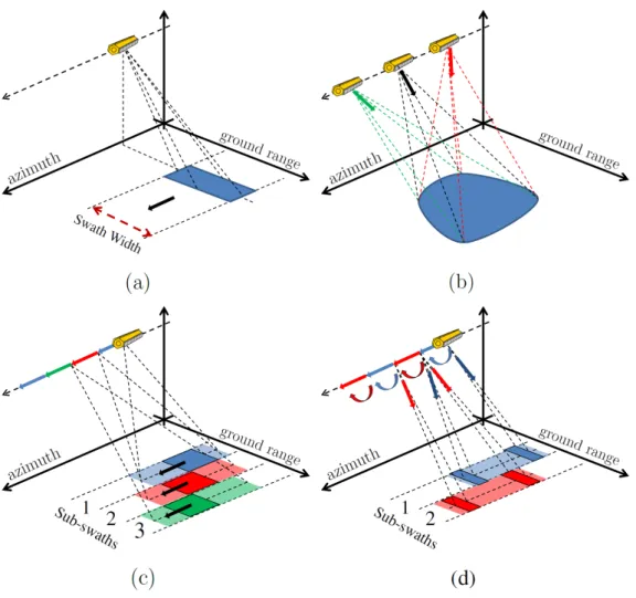
Radar sensors for remote sensing applications can be divided into three classes: scat-terometers, altimeters, and imaging radars.
• Scatterometers are radar devices designed to determine the backscatter level of
the illuminated area [1], defined as the portion of the transmitted electromagnetic signal that the target redirects back towards the radar antenna. Backscatter data from scatterometers are applied to the study of vegetation, polar ice, soil moisture, and ocean current tracking.
• Radar altimeters are used to measure the altitude above the terrain beneath the
sensor platform by measuring the time delay that occurs between the transmission and reception times of the reflected radio wave.
Table 1.1.: Summary of typical carrier frequencies for remote sensing radar systems. Radar Frequencies
Denomination Frequency Wavelength
[GHz] [cm] P 0.23-1 30-130 L 1-2 15-30 S 2-4 7.5-15 C 4-8 3.75-7.5 X 8-12 2.5-3.75 Ku 12-18 1.67-2.5 K 18-27 1.11-1.67 Ka 27-40 0.75-1.11 V 40-75 0.4-0.75 W 75-110 0.27-0.4
• Imaging radars are able to map the returning electromagnetic waves from
on-ground objects onto a two-dimensional plane. The intensity of the backscattered signals can be properly composed to obtain an optical-like image of the illuminated ground: the higher the received signal is, the brighter the corresponding pixel in-side the final image will be. Moreover, the information about the phase of the reflected wave is available as well, containing information on the distance of the illuminated objects from the sensor. Modern imaging radar techniques are based on the Synthetic Aperture Radar (SAR) principle, which exploits the motion of the radar antenna over a defined ground region, in order to obtain a finer resolution. Given their characteristics, SAR images are suitable not only for simple imaging pur-poses, but for a variety of different scientific applications as well, among which are:
• SAR interferometry: by exploiting the phase difference between two or more SAR images acquired at different sensor positions, it is possible to generate elevation maps of the surface [2]. If a series of images subsequently acquired is considered, it is possible to detect the changes in time of the position of the illuminated targets on
ground, allowing to monitor subsidence and deformation phenomena (differential
interferometry) [3].
• SAR tomography: SAR interferometry has the limitation of retrieving the simple phase center of all the targets on ground within a resolution cell, which does not always coincide with the terrain topograpy (e.g. in the presence of vegetation or urban areas). SAR tomography was born in order to fill this gap, by estimating the
1.2 A Historical Overview of Spaceborne SAR
vertical distribution of the scatterers, by means of repeat-pass acquisitions over the same area from slightly different positions [4].
• SAR polarimetry: it is based on the combination of SAR images acquired over the same ground area with different wave polarizations. In this way, different backscattering mechanisms can be characterized and associated to several physical processes [5], [6].
1.2. A Historical Overview of Spaceborne SAR
The birth of radar dates back to the beginning of the twentieth century. In 1904, build-ing on Heinrich Hertz’s discovery that electromagnetic waves were reflected from
metal-lic surfaces [7], Christian Hülsmeyer invented the so called Telemobiloscope, able to
detect the presence of distant objects using electromagnetic waves [8]. However, the working principle of radar can even be found in nature. Bats, for example, utilize a nat-uralSONAR(SOund Navigation And Ranging), being able to locate animals by emitting calls out in the environment and listening to those calls which return from objects nearby.
The termRADARwas coined in 1939 by the Unites States Navy, as the acronym ofRAdio
Detection And Ranging, becoming later on a common noun. During World War II, radar started to be used for object detection purposes, and later on for civilian applications as well, such as traffic and weather monitoring.
After the second World War, the SLAR (Side Looking Airborne Radar) was invented,
aiming at imaging ground areas from airborne platforms. Flying along a defined path (along track dimension), it was able to acquire images by pointing the antenna beam perpendicularly to the flight direction (across track dimension). Its resolution, defined as the ability to distinguish between two targets on ground, depends on the transmitted pulse bandwidth in the across track direction, and on the beamwidth of the radar antenna in the along track direction.
At the beginning of the 1950s the need for higher-resolution images led to the develop-ment of Synthetic Aperture Radar (SAR). In 1951, Carl A. Wiley observed that a finer resolution in the along track dimension can be obtained by exploiting the motion of the radar antenna over a target region [9]. The principle resides in synthesizing an antenna of large dimensions (on the order of kilometers) in the along track dimension, by properly combining the information coming from each target on ground, obtained at different po-sitions of the radar sensor. Since then, SAR has been widely recognized as a paramount mean for remote sensing applications, and an increasing number of airborne and space-borne missions has been developed throughout the years, significantly improving the resolution and quality of the delivered images.
Figure 1.1.: (a) NASA’s Seasat satellite, launched in 1978. (b) Seasat SAR image over
the Teepee Park, Yukon, Canada. Acquired on July21st, 1978, by NASA.
1.1) [10]. Launched in 1978, it was mounted with an L-band radar antenna, designed to monitor oceanographic phenomena on a global scale, such as sea surface winds and tem-perature, wave heights, and sea ice features. Later on, a series of L-band SAR sensors were mounted on-board the Space Shuttle, leading to the Shuttle Imaging Radar missions SIR-A (1981) [11], [12] and SIR-B (1984) [13].
The Japanese Space Agency (JAXA) further developed L-band spaceborne SAR sensors, launching JERS-1 in 1992, ALOS in 2006, and ALOS-2 in 2014 [14], [15].
The first remote sensing satellite developed by the European Space Angency (ESA) was ERS-1 [16]. Launched in 1991, it was equipped with a C-band SAR antenna and oper-ated until 2000. The continuity of acquired data was assured first by its follow-up twin satellite ERS-2, launched in 1995, and then by ENVISAT, launched in 2002 and in op-eration until 2012 [17] [18]. The ENVISAT satellite mounted nine different instruments for the observation of the Earth, among which the ASAR C-band active antenna array, allowed to electronically steer the antenna beam in both transmitting and receiving di-rections. In 2014 and 2016, ESA launched Sentinel-1A and Sentinel-1B, respectively, as part of the Copernicus Program [19]. These two satellites are equipped with a SAR an-tenna operating at C band, and provide continuity of data after ENVISAT, with enhanced capabilities in terms of revisit time and coverage.
The Canadian Space Agency launched RADARSAT-1 and RADARSAT-2 in 1995 and 2007, respectively: two C-band SAR satellites, whose orbit is optimized for regularly observing the Arctic up to the pole, at the disadvantage of loosing the illumination of the central areas of Antarctica [20], [21].
1.3 Motivation of the Work
Another milestone in spaceborne SAR is represented by the SIR-C/X-SAR missions, de-veloped in a joint venture between NASA JPL and a European consortium of the German Aerospace Center (DLR) and the Italian Space Agency (ASI) [22]. The instrument, with multi-bandwidth capabilities (L, C, and X bands), was flown on two Space Shuttle flights in April and October 1994, opening the way for the development of the Shuttle Radar Topography Mission (SRTM) in 2000 [23]. Both NASA and DLR took part in that mis-sion, whose objective was the generation of an Earth Digital Elevation Model (DEM) on
a near global scale, from56◦ S to60◦ N latitudes.
In June 2007, TerraSAR-X was launched: an imaging radar Earth observation satel-lite, developed under a public-private-partnership between DLR and Airbus Defence & Space. The satellite operates at X band and is able to acquire high-quality SAR images with a resolution of up to 1 m [24].
A twin satellite, TanDEM-X, was then launched in 2010, officially starting, together with TerraSAR-X, the bistatic TanDEM-X mission. Flying in a close-orbit configuration, both satellites act as single-pass interferometer, allowing for the acquisition of high-resolution interferograms [25]. The generation of a global DEM, completed in 2016, was the main objective of the TanDEM-X mission and the generation of an additional change-DEM layer is foreseen for 2020.
Other on-going spaceborne SAR missions are the Italian X-band constellation of four satellites COSMO-SkyMed [26], the first military-civil system for Earth observation, and the Korean KOMPSAT-5 [27], an X-band SAR mission launched in 2013.
1.3. Motivation of the Work
Radar backscatter represents a fundamental quantity in radar measurements. Its pro-perties change depending on several factors, such as sensor parameters (e.g. frequency and polarization), soil conditions, and surface roughness. Moreover, it is influenced by atmospheric conditions, on-ground vegetation, topographic characteristics of the illumi-nated ground area, and acquisition geometry.
High accuracy in commanding, processing and system performance is required in order to provide high quality SAR images. The accurate knowledge of backscatter represents a valuable input for an optimized operation of the whole SAR system.
As an example, one can take into account the TerraSAR-X and TanDEM-X satellites, where no automatic adaptation of the commanding radar parameters is performed on-board during a data take. Acquisitions are commanded with pre-defined receiver gain setting and no automatic gain control is performed. For known backscatter character-istics of a requested SAR scene, the receiver gain can be suitably adapted to mitigate clipping or signal saturation [24].
backscatter is necessary for the prediction of SAR performance, and therefore for the optimization of the design strategy. An example is given by the design of the future Tandem-L mission, which will make use of innovative digital beamforming techniques to achieve high-resolution wide swath imaging [28], [29].
Backscatter information is widely used for a number of scientific applications as well. For example, backscatter levels can be related to biomass using polarimetry [30], or serve as input for retrieving snow mass from radar images [31].
With the availability of X-band SAR data for scientific purposes, the investigation of X-band backscatter from spaceborne platforms has become a highly interesting research topic in the last years. Furthermore, the global coverage provided by the TanDEM-X mission, together with the availability of a fine-scale land cover classification, allows for the generation an up-to-date data set of radar backscatter models at X band, opening the door for the generation of high resolution X-band backscatter maps on a global scale, which represents a highly interesting topic for both the scientific community and the de-sign of future SAR missions.
The main goal of this work is to exploit the global TanDEM-X data set to statistically model radar backscatter at X band, considering different acquisition parameters and land cover types, and to provide the remote sensing community with an up-to-date data base of models, describing the Earth’s reflectivity at X band.
The backscatter dependency on season and geographic location has been investigated as well and a proper selection of the input observations allows to derive specific models, which locally increase the final accuracy.
Moreover, particular attention has been focused on the Greenland Ice Sheet, which rep-resents a highly interesting topic for the scientific community. In fact, melt phenomena have strongly increased in the last years, leading to modifications in the characteristics of the snow pack. A better knowledge of the Ice Sheet can substantially contribute to a better understanding of the arctic and its response to climate change. The unique inter-ferometric signature of the bistatic TanDEM-X system has allowed for the development of a method to characterize different snow facies and subsequently refine the derived backscatter models, depending on the characteristics of the snow pack.
Finally, the availability of the global TanDEM-X SAR data set, together with the derived data base of backscatter models, allows for the derivation of a global backscatter map at X band, a key-quantity for the design of future SAR missions.
1.4. Thesis Structure
1.5 Original Contribution of the Thesis
• Basic concepts on electromagnetic waves, radar backscatter, SAR image
forma-tion, and SAR interferometry are summarized in chapters 2 and 3. This theoretical part is not meant as a comprehensive compendium on the proposed subjects, but rather as a summary of all necessary concepts for understanding the developed work.
• An overview of the TanDEM-X mission is presented in chapter 4, together with the
description of the global data set of derived quicklook images. Such data serves as input for the application, testing, and validation of the developed algorithms.
• The newly developed backscatter modeling algorithm is presented in chapter 5,
together with a discussion on the sources of error and on the proposed models ver-ification approach. Moreover, the impact of backscatter seasonal changes within the modeling process is addressed as well and a possible solution is proposed. The attention is then focused on rain forests, which represent a widely used target for SAR calibration purposes. Here, an analysis of backscatter behavior depending on acquisition daytime and geometry is presented and discussed.
• Chapter 6 is dedicated to the Greenland Ice Sheet. The presence of different kinds
of snow cover and the lack of an appropriate ground classification map led to the development of the proposed algorithm for the identification of different snow fa-cies. Based on the derived two-dimensional snow facies map, ad-hoc backscatter models are derived for each snow facies, separately, and the radar wave penetration depth into the ice sheet is estimated as well.
• Chapter 7 presents a possible application of a global data base of backscatter
mod-els, consisting in the generation of large-scale backscatter maps. Here, the de-veloped algorithm for the equalization of independent input backscatter data to a common reference incidence angle is presented, together with their mosaicking on a common output grid. An iterative algorithm is finally implemented to fill remaining gaps due to missing input data.
• Finally, conclusions and future work are summarized in chapter 8, while a data
base of polynomial backscatter models and statistical values, obtained from the global TanDEM-X mission data, is provided in appendix A.
1.5. Original Contribution of the Thesis
This thesis is the result of the work carried out at the Microwaves and Radar Insti-tute (HR) of the German Aerospace Center (DLR), Germany. Its original contribution comprises:
• The extraction and processing of the entire global data set of TanDEM-X quick-look images (lower resolution images derived by averaging full resolution ones), together with the derivation of additional quantities, such as the signal-to-noise ratio (SNR) or the terrain predominant slope, which are necessary for the develop-ment of the presented algorithms and analysis.
• The development of a new algorithm for modeling radar backscatter. The unique
amount of data made available by the TanDEM-X mission has provided the mo-tivation to model backscatter by concentrating on the statistics provided by the SAR data itself, rather than building a theoretical model, based on the physical principles of radar backscattering mechanisms.
• The generation of an up-to-date data base of backscatter models for X band,
cov-ering different kinds of land cover at a global scale.
• The seasonal and geographic dependency of the backscatter has been analyzed as
well and backscatter models have been separately derived for different seasons. In particular, the analysis of such a dependency has been focused on the tropical rain forest, which, given its isotropic characteristics, is commonly used as a reference distributed target for sensor calibration purposes.
• A dedicated analysis of the Greenland Ice Sheet, aimed at locating different snow
facies, as seen by TanDEM-X. A classification approach has been developed taking into account the interferometric signature of TanDEM-X data.
The derived snow facies are used for two main purposes:
– To provide a set of backscatter models, depending of the characteristics of
the snow pack,
– To estimate the two-way X-band penetration depth into the ice sheet.
• Finally, an algorithm for the generation of backscatter maps has been developed
and represents a possible application of the derived backscatter models data base. Moreover, the research work presented in this thesis can also be seen as an ignition for the development of the global TanDEM-X Forest/Non-Forest Map product, derived from the global data set of TanDEM-X bistatic acquisitions [32], and of the related on-going activities at the institute, aimed at developing novel multi-sensor approaches for monitoring deforestation [33].
It is also worth mentioning that the derived snow facies map is the first information product on a continental scale, generated by an interferometric spaceborne SAR mission beyond the standard digital elevation model (DEM).
2. Theoretical Background
2.1. Electromagnetic Waves
To fully understand radar backscattering mechanisms, it is important to recall the Elec-tromagnetic (EM) Wave theory basics and the way in which such waves interact with materials. An exhaustive compendium of the subject can be found in [34] and [1]. This section provides a short overview of EM waves, focusing on EM plane waves and some of their properties, which are useful for the understanding of the present work. The con-tent of this section is confined to lossless media, where waves do not suffer from any attenuation. A more detailed description of propagation in lossy media can be found in [35] and [1].
2.1.1. Electromagnetic Plane Waves
An EM wave is the result of a time-varying electric field which induces a magnetic field or, vice versa, of a time-varying magnetic field which induces an electric one. Waves can propagate both in lossless mediums, without attenuation, or in lossy ones, where part of the wave’s energy is dissipated into heat. Materials in general are characterized by four constitutive parameters [1]:
• the conductivityσc,
• the volume charge densityρv,
• the magnetic permeabilityµmag,
• the electrical permittivityε0ε0, whereε0 is the permittivity of free space and ε
0
is the permittivity of the material relative to that of free space.
If a wave is generated by a punctiform or localized source, it expands in all directions with the same velocity, leading to the generation of a spherical wave. If the wave’s front is observed at a very large distance from the source (in the so-called far field region), it appears approximately planar, with identical properties all over the plane tangent to the wavefront. Such waves are called plane waves and they can be described in a Cartesian
coordinate system(x, y, z).
The way in which electric and magnetic fields are generated and altered by each other and by currents and charges is described by Maxwell’s differential equations, which, in a homogeneous and isotropic medium, are given by:
∇ ·E = ρv ε0ε0 (Gauss’s law), (2.1) ∇ ×E =−µmag ∂H ∂t (Faraday’s law), (2.2)
∇ ·H= 0 (Gauss’s law for magnetism), (2.3)
∇ ×H=J+ε0ε0
∂E
∂t (Ampère’s law), (2.4)
where Eis the electric field intensity, Hthe magnetic field intensity, and J the current
density flowing through the medium.
If the time variation of the electric and magnetic fields (E and H) is sinusoidal with
angular frequencyω,EandHcan be represented with vector phasors which depend on
(x, y, z)only. In this case, the vector phasor of the electric field E(x, y, z)is related to the instantaneous electric field at the timet,E(x, y, z;t), by:
E(x, y, z;t) = <
E(x, y, z)ejωt, (2.5)
wherej =√−1.
Differentiation in the time domain corresponds to a multiplication by jω in the phasor
domain. Maxwell’s equations in the phasor domain therefore become:
∇ ·E= 0, (2.6)
∇ ×E=−jωµmagH, (2.7)
∇ ·H= 0, (2.8)
∇ ×H=jωεε0E, (2.9)
whereεis the complex dielectric constant, defined as [1]:
ε=ε0 −j σc ωε0
. (2.10)
The explicit solutions forEandHcan be derived from Maxwell’s equations as presented
in [34], obtaining the homogeneous wave equation forEandHas:
∇2E+γ2E= 0, (2.11)
∇2H+γ2H= 0, (2.12)
whereγrepresents the propagation constant and is defined as:
2.1 Electromagnetic Waves
Since both (2.11) and (2.12) are of the same form, the solution of the wave equation is
now derived forEonly. The same considerations stand forHas well.
By considering a lossless medium, whereε=ε0, and by defining the wavenumberkas:
k =ω q
µmagε
0
ε0, (2.14)
(2.11) can be written as:
∇2E+k2E= 0. (2.15)
In Cartesian coordinates the electric field phasor can be decomposed as:
E=ˆxEx+yˆEy+ˆzEz, (2.16)
where(xˆ,ˆy,ˆz)is the Cartesian unit vector, and the Laplacian ofEis given by:
∇2E= ∂ 2 ∂x2 + ∂2 ∂y2 + ∂2 ∂z2 E. (2.17)
By substituting (2.17) into (2.11), the following relationship is obtained for theEx
com-ponent: ∂2 ∂x2 + ∂2 ∂y2 + ∂2 ∂z2 +k 2 Ex = 0. (2.18)
Analogous expressions are valid forEy andEz, which means that, if an infinite plane is
considered, both the electric and magnetic fields components belonging to it are charac-terized by uniform properties and their derivatives are therefore equal to zero. Assuming
such a plane to be the(x, y)one, (2.18) becomes:
∂2E x
∂z2 +k 2E
x= 0. (2.19)
The same applies to Ey, Hx, and Hy. For the remaining components it is valid that
Ez =Hz = 0, leading to the conclusion that the direction of propagation of a plane wave
is characterized by the absence of electric and magnetic field components. The general solution of the ordinary differential equation in (2.19) can be derived by applying the
boundary conditions, as presented in [1]. For the phasorExit can be obtained that:
Ex(z) =Ex0+e
−jkz+E− x0e
jkz, (2.20)
where Ex0+ and Ex0− are two constants, whose value can be determined by applying the
boundary conditions. The term e−jkz identifies a wave travelling in the +z direction,
while the term ejkz represents a wave travelling in the−z one. The same kind of
solu-tion can be derived for the otherE andHcomponents. The electric and magnetic field
Figure 2.1.: Propagation of a TEM wave, decomposed into its electric (E) and magnetic
(H) field components, which are perpendicular to the propagation’s direction
along thezaxis. λrepresents the wavelength.
wave, identifying a so called transverse electromagnetic (TEM) wave, whose represen-tation is shown in Fig. 2.1. The direction of propagation of such a wave is defined by the
cross productE×H, being the latter oriented accordingly and parallel to thezaxis.
As-suming to haveEcomponents alongxonly (Ey = 0) and travelling in the+z direction
only, (2.20) becomes:
E(z) = ˆxEx0+e−jkz, (2.21)
and, by applying (2.7), the associated magnetic field is:
H(z) = ˆyHy0+e−jkz, (2.22)
where:
Hy0+ = k ωµmag
Ex0+. (2.23)
For a lossless medium, theintrinsic impedancecan now be defined as the ratio between
the magnitude of the electric and magnetic fields as:
η = E + x0 Hy+0 = ωµmag k = r µmag ε0ε 0 . (2.24)
The E and H components on the z plane, perpendicular to the propagation direction,
show the same dependency on time t, by mean that they both reach their maximum or
minimum amplitudes at the same time. This is a typical characteristic of waves in lossless
media and bothE andHare said to bein phase. Hence, thephase velocityof the wave
2.1 Electromagnetic Waves vp = ω k = 1 p µmagε 0 ε0 , (2.25)
and the wavelength as:
λ = 2π k =
vp
f , (2.26)
wheref =ω/2πis the frequency.
2.1.2. Electromagnetic Power Density
The energy flow carried by an electromagnetic wave per unit areaSEW(t)is described
by thePoynting vector:
SEW(t) = E(t)×H(t). (2.27)
SEW(t)is perpendicular toE(t)andH(t), and oriented accordingly to the wave’s
propa-gation direction. From (2.27) thetime-averaged Poynting vectorper unit timeT for EM
planar waves is derived as [34]:
hSEWi= 1 T Z T 0 SEW(t)dt= 1 2< E×H∗. (2.28)
By assuming that the wave flows through an aperture of areaA, the total powerPtot that
is intercepted by the aperture is derived by integratinghSEWiover the surfaceA:
Ptot =
Z
A
hSEWi ·nˆdA, (2.29)
wherenˆrepresents the normal to the surface.
2.1.3. Wave Polarization
Polarization is a characteristic of electromagnetic waves and indicates the direction of oscillation of the electric field during the wave’s propagation in space and time. The magnetic field is consequently polarized in the orthogonal direction with respect to the electric field and to the propagation’s direction. If the direction of oscillation of the
electric field randomly changes, such wave is said to be unpolarized. For plane waves,
three types of polarization can be distinguished:
• Linear polarization: the electric field oscillates in one direction only, describing a linear segment in time on the plain in which it resides. Moreover, the plane
Figure 2.2.: Polarization of an electromagnetic wave. The electric fieldEis depicted for: (a) unpolarized wave, (b) linearly polarized wave, (c) left-hand circularly (LHC) polarized wave [36].
of incidence is defined as the plane to which the direction of propagation of the incident wave and the normal to the boundary belong to. Linearly polarized waves can be further classified ashorizontal, if the electrical field is perpendicular to such a plane, orvertical, if the electrical field is parallel to it.
• Circular Polarization: the electric field describes a circle in time on the plain in
which it resides. It can be distinguished between left-hand circular polarization
(LHC), if the electric field describes in time a clockwise circle, andright-hand
cir-cularpolarization (RHC), if the electric field describes in time a counterclockwise circle.
• Elliptical Polarization: the electric field describes an ellipse in time in the plane
in which it resides. Also in this case it is possible to distinguish betweenleft-hand
(LHE) andright-hand elliptical(RHE) polarization.
A summary of different polarization is shown in Fig. 2.2.
2.1.4. Wave Reflection and Transmission at the Interface
Consider now two different homogeneous and lossless dielectric media, with perme-abilityµmag,0 and relative permittivityε
0
1 andε
0
2, respectively. The considered media are
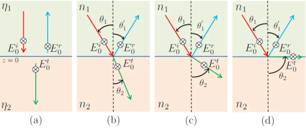
separated by a planar interface located atz = 0, as presented in Fig. 2.3 (a). Assume to
have a TEM wave, which propagates within medium 1 in the direction perpendicular to
thez = 0plain, towards the interface with medium 2. The incident electric and magnetic
fields are identified asEiandHi. At the moment of the interaction between the incident
wave and the interface (z= 0), a portion of the incident electric and magnetic fields (E0i
andHi
2.1 Electromagnetic Waves
Figure 2.3.: EM wave reflection and transmission at the interface between medium 1
(intrinsic impedanceη1 and index of refractionn1) and medium 2 (intrinsic
impedanceη2and index of refractionn2). (a) Normal incidence. (b) Inward
refraction. (c) Outward refraction. (d) critical angle (no transmission).
medium 2 (Et
0andH0t). The mechanisms of reflection and transmission are regulated by
the Fresnel laws for normal incidence, which state that:
ρc = E0r Ei 0 = η2−η1 η2+η1 , (2.30) τc = Et 0 Ei 0 = 2η2 η2+η1 , (2.31)
whereη1andη2are respectively the intrinsic impedances of medium 1 and 2, andρcand
τcidentify the Fresnel reflection and transmission coefficients.
If the incident wave meets the interface between the two media with a certain angleθ1, as
in Fig. 2.3 (b) - 2.3 (d), a portion if it is reflected back into medium 1, forming an angle
θ10 with the normal to the boundary which is related toθ1by the Snell’s law of reflection:
θ1 =θ
0
1; (2.32)
while part of it will be transmitted into medium 2 changing its direction accordingly to Snell’s law of refraction:
sinθ2 sinθ1 = vp2 vp1 = s ε01 ε02, (2.33)
wherevp1 andvp2 are the phase velocities characterizing medium 1 and 2, respectively.
ratio between the phase velocity in free space, which for a lossless medium of
permit-tivity ε0ε0 can be described using the speed of light vlux, and the phase velocity in the
medium itself: nc= vlux vp = s µmag,0ε 0 ε0 µmag,0ε0 = √ ε0. (2.34)
ncquantifies the decrease of the wave’s propagation velocity when it travels in a medium,
with respect to free space. If the indices of refractionnc
1andnc2are associated to medium 1 and 2, respectively, (2.33) becomes:
sinθ2 sinθ1 = vp2 vp1 = n c 1 nc 2 . (2.35)
In particular, one can refer to inward refraction if nc1 < nc2, and therefore θ1 > θ2
(Fig. 2.3 (b)), and tooutward refractionifnc
1 > nc2, leading toθ1 < θ2 (Fig. 2.3 (c)). A particular case happens whenθ2 =π/2, calledcritical angleθc. In this case, the refracted wave travels on the interface between the two media, and no energy is transmitted into medium 2, as shown in Fig. 2.3 (d).
2.2. Radar Backscattering
In the following section the fundamental concepts of radar backscattering mechanisms, such as the scattering matrix and radar backscattering from a point or distributed target, are discussed. The radar equation is introduced, together with basic concepts of surface
and volume scattering. The concept of speckle will be discussed later on in chapter 3,
since its interpretation is directly related to SAR images.
2.2.1. Scattering Matrix
Consider an EM plane wave, polarized in both horizontal and vertical directions, illu-minating a small scattering object in the far-field region. The transmitted and received
electric fieldsEtandErcan be decomposed in the following way:
Et = ˆvtEvt+ ˆhtEht,
Er = ˆvrErt+ ˆhrEhr, (2.36)
where the unit vectors hˆt, hˆr, vˆt, and vˆr identify the directions of the horizontal and
2.2 Radar Backscattering
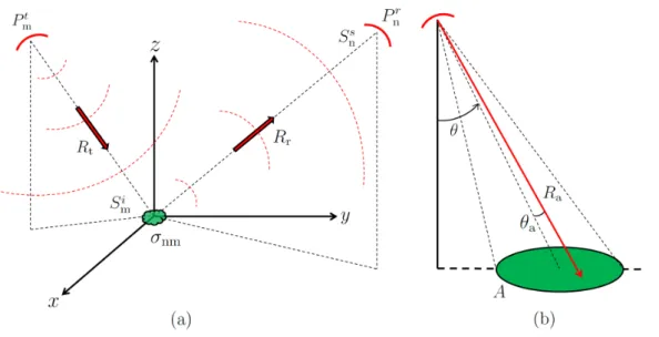
Figure 2.4.: (a) Reference geometry for the computation of the radar equation. (b)
Illu-mination geometry for a distributed target of areaA.
Er v Ehr = e−jkRr Rr svv svh shv shh Et v Eht (2.37)
whereRris the distance between the receiver and the illuminated object,(e−jkRr/Rr)is the spherical propagation factor, and the matrix
s= svv svh shv shh (2.38)
is called scattering matrix. It contains the differently polarized components of the ob-ject’s scattering amplitude, where, as stated in [37], for the principle of reciprocity,
svh =shv.
2.2.2. Scattering from a Point Target
A point target is an object of small dimensions compared to the angular resolution of the radar, which means that the solid angle that it subtends is much smaller than the one subtended by the antenna beam.
Consider now the radar bistatic configuration in Fig. 2.4, composed of a transmitting
m-polarized antenna, where the m-index can either correspond to linear horizontal (h
-index) or vertical (v-index) polarization, and a receivingn-polarized one. A single point
transmitting antenna, which is then scattered back along different directions. Only a
portion of the reradiatedn-polarized energy is intercepted by the receiving antenna. This
process is described by thepoint target bistatic radar equation[38]:
Pnr = P t mGtGrλ2 (4π)3R2 tRr2 σnm (2.39) wherePr
n is the received n-polarized power,Pmt is the transmittedm-polarized power,Gt
andGr the transmitting and receiving antenna gains,Rr the distance between the target
and the receiving antenna, andσnmtheradar cross section. In case of a monostatic radar,
whereGt =Gr=GandRt =Rr=R, (2.39) becomes:
Pnr = P
t
mG2λ2
(4π)3R4σnm. (2.40)
The radar cross sectionσnmrepresents the strength, with which the target redirects back
the illuminating energy and is defined as in [38]:
σnm = lim Rr→∞ 4πR2r S s n Si m , (2.41)
whereSns is the scattered power density at the location of the receiving antenna andSmi
is the power density illuminating the target. The limitRr → ∞underlines the fact that
the scattered power densitySs
n is measured in the far-field region, where the wave front
can be considered to be planar. As presented in [1], the radar cross-section in (2.41) can be expressed in terms of scattering amplitude, introduced in section 2.2.1, as:
σnm= 4π|snm|2. (2.42)
2.2.3. Scattering from a Distributed Target
Distributed targets are extended targets where the contribution at the receiving antenna is given by the coherent sum of multiple reflections and where there is no predominant scattering mechanism within the resolution cell. (2.40) can therefore be extended to this
case by integrating over the illuminated areaA:
Pnr(θ) = Z Z Aσ PmtG2(θa, φa)λ2 (4π)3R4 a σnm0 dAσ, (2.43)
where θ is the incidence angle of the boresight direction of the transmitting antenna
andφa is the squint angle. (θa, φa)define the direction to a point insideA with respect
to the antenna boresight direction, and Ra is the distance between the point and the
antenna. σ0
2.2 Radar Backscattering
Figure 2.5.: Reference geometry for the incidence angle θ and for the local incidence
angleθl.
backscattering coefficient), defined as the radar cross sectionσnmof a distributed target of areaAσ, normalized with respect toAσ itself:
σ0nm=σnm/Aσ. (2.44)
Moreover, the radar backscatter can be defined as the direct ratio between the scattered
power and the incident power at ground level; in this case it is identified asβnmand the
backscattering coefficient can be expressed in terms of reflectivity per unit area in slant rangeAβ. It is calledradar brightnessβnm0 and is related toσnm0 by:
βnm0 = βnm Aβ = σ 0 nm sin(θl) , (2.45)
where θl is the local incidence angle and describes the angle between the radar wave
incident direction and the normal direction to the scattering surface, as depicted in Fig. 2.5. In case of flat Earth,θlcoincides with the incidence angleθ.
Finally, it is also possible to express the backscattering coefficient in terms of unit area
perpendicular to the antenna beamAγ. In such a case, it is denoted asγnm0 and given by:
γnm0 =βnm0 Aβ Aγ
=βnm0 tanθl. (2.46)
The reference geometry for flat Earth displaying the backscatter normalization areas
Figure 2.6.: Reference geometry for flat Earth displaying the backscatter normalization areasAσ,Aγ, andAβ.
Figure 2.7.: (a) Surface scattering from a random surface, characterized by single and multiple scattering. (b) Volume scattering from vegetation canopy. (c) Sur-face and volume scattering from snow-covered soil.
2.2.4. Surface and Volume Scattering
The received backscattered radar signal is generally given by eithersurfaceorvolume
scatteringmechanisms, or by a combination of both of them [1]:
• Surface scatteringdenotes the reradiated signal from the air-soil interface. It can
be divided intosingleormultiplescattering, depending on whether the signal is
di-rectly sent back towards the radar antenna or it involves multiple reflections against other targets. An example is presented in Fig. 2.7 (a).
• Volume scatteringoccurs when the reradiated signal is the sum of the contributions from many individuals scatterers located at different positions within a certain vol-ume, e.g. between the soil and the top of the canopy, as presented in Fig. 2.7 (b). Volume scattering is influenced by several factors, such as density, three-dimensional orientation, shape of the targets, their dielectric composition, and the
2.2 Radar Backscattering
radar wavelength.
• Surface and volume scattering is a combination of both scattering mechanisms. Snow-covered areas are a typical example of where both surface and volume scat-tering mechanisms interact with each other, as shown in Fig. 2.7 (c). The snow surface directly contributes with surface scattering, while the snow layer is char-acterized by the presence of ice crystals which can act as reflectors, contributing to volume scattering. Depending on the conditions of the snow pack and on the wavelength, the EM wave can penetrate into the snow layer and reach the ground, where a further backscattering occurs.
2.2.5. Chapter Remarks
This chapter is meant to provide the reader with basic background concepts on elec-tromagnetic plane waves and radar backscatter, needed for the understanding of the fol-lowing chapters.
In particular, the reader should now be aware of the main mechanisms regulating the propagation of a TEM wave, characterized by electric and magnetic field components perpendicular to each other and to the direction of propagation.
The concepts of wave polarization and wave reflection and transmission at an interface become of fundamental importance for understanding radar backscatter and its proper-ties.
This topic has been introduced by defining the scattering matrix and the concept of radar cross section, which quantifies the strength with which a target redirects the illuminating energy towards the receiving antenna.
Given a certain transmitted power, the antenna gain, and the acquisition geometry, the received power is regulated by the radar equation. The latter has been formulated for both a point and a distributed target. Moreover, for distributed targets, the backscattering coefficients for different projections have been derived as well.
Finally, the chapter is concluded with a brief introduction on different kinds of scatter-ing mechanisms, divided into surface, volume, and a combination of surface and volume scattering.
In this chapter the fundamental principles ofSynthetic Aperture Radarand SAR inter-ferometryare discussed.
In section 3.1, the SAR image formation is presented, starting from the acquisition ge-ometry, until the final image focusing, absolute calibration, and geocoding. Exhaustive contributions on the subject can be found in [39], [35], [40], and [41].
In section 3.2, the attention is focused on the descriptionacross-track interferometry,
which allows to retrieve a digital elevation model (DEM) starting from a pair of SAR
images, acquired from two slightly different positions. A detailed compendium on the topic can be found in [2].
3.1. SAR Image Formation
3.1.1. Acquisition Geometry and Resolution
ASynthetic Aperture Radaris a side-looking radar used in remote sensing for imaging purposes. It is normally mounted on either airborne or spaceborne platforms, sending
electromagnetic pulses at a definedpulse repetition frequency(PRF). The acquisition
ge-ometry is displayed in Fig. 3.1, wherexidentifies the along-track dimension (azimuth),y
the across-track dimension (ground range), andzthe sensor hight direction. The sensor
is a radar antenna with azimuth length La and flies along the azimuth dimension. The
slant range(or simplyrange) dimension identifies the direction between the sensor and
the target on ground. The slant range resolution ρrg, defined as the minimum distance
that allows to correctly resolve two separate targets, is proportional to the pulse duration
in timeτrgand inversely proportional to the bandwidthBrgof the transmitted signal:
ρrg = vluxτrg 2 = vlux 2Brg , (3.1)
Once the slant range resolutionρrghas been defined, it is possible to derive the resolution
on ground as: ρg = ρrg sin(θi) = ρrg sin(θ−α) = vlux 2Brgsin(θ−α) , (3.2)
whereθiis the incidence angle with respect to the ground,θis the one with respect to the
3.1 SAR Image Formation
Figure 3.1.: Reference geometry for a SAR acquisition.
is presented in Fig. 3.4 (a).
The transmitted pulse d(τ) is typically a complex chirp, characterized by a constant
amplitude in the time domain and given by:
d(τ) = ejπkrτ2rect(τ /τ
rg), (3.3)
where kr is the chirp rate and τ is the slant range time. An example is given in Fig.
3.2. Such an impulse is linearly frequency modulated, and it allows to spread the signal power on a wider time window, avoiding the necessity of increased transmitted power for assuring a high resolution.
The angular resolution in azimuth of a side-looking radar θaz (shown in Fig. 3.1)
depends on the antenna beam width and is given by:
θaz =
λ La
. (3.4)
By increasing the observation time of an object, a higher azimuth resolution ρaz can be
achieved by exploiting the concept of thesynthetic aperture Lsa, which is defined as the
distance that the sensor covers during a complete acquisition with durationTo. It is given
Figure 3.2.: Example of sampled complex chirp pulse.
Lsa =
λR0
La
, (3.5)
whereR0 represents the minimum distance between the sensor and the closest approach
to the target (zero Dopplerdistance). In this way, the backscattered signal coming from
an on-ground object is recorded during the whole observation time To and then
recon-structed by means of a coherent sum of all the energy contributions spread alongTo. This
operation, calledazimuth focusing, is explained in section 3.1.3.
The angular resolutionθsa corresponding to the synthetic apertureLsa can be evaluated
as:
θsa =
λ 2Lsa
, (3.6)
where factor 2 takes into account the two-way path of the electromagnetic wave. Hence,
the enhanced azimuth resolutionρaz is given by:
ρaz =θsaR0 =
La
2 . (3.7)
By assuming now a rectilinear geometry, where the sensor’s orbit is considered to be
linear, and thestart-stopapproximation, where both sensor and scatterers remain steady
3.1 SAR Image Formation
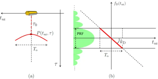
Figure 3.3.: (a) The hodograph: the signature of a point target left within the acquired SAR data and subjected to range migration. (b) Doppler history of a point target in the azimuth time/Doppler frequency plane.
the acquired data matrixP(taz, τ) (calledhodograph) is simplified in Fig. 3.3 (a). For
each sensor position along the azimuth time dimensiontaz, the range timeτ between the
sensor andP(taz, τ)is given by:
τ = 2 vlux R(taz). (3.8) R(taz)is defined as: R(taz) = q R2 0+ (vstaz)2, (3.9)
where vs is the sensor speed and R0 = (vlux/2)τ0, being τ0 the range time associated
to the zero Doppler position of the target. (3.9) identifies an hyperbole, whose summit corresponds to the target position in SAR geometry. The shift of a target’s signature in
slant range depending on the sensor’s azimuth position is also known asrange migration.
The backscattered energy from a target, spread over the hodograph, is used to reconstruct
the target by applying theazimuth focusing, as explained in section 3.1.4.
By using a Taylor approximation, (3.9) can be simplified with a parabolic function as:
R(taz)'R0+
v2 s
2R0
t2az. (3.10)
The phase in azimuth of the impulse response from the considered target can now be obtained from the hodograph as: