Measuring Hotel Performance:
Toward more rigorous evidence in both scope and method
Abstract
This paper extends the literature on hotel performance in terms of both scope and method. We introduce a model that accounts for heterogeneity in a flexible way and allows for the measurement of both efficiency and productivity. The model also accounts for the endogeneity problem in inputs and the issue of unobserved prices. We use a large sample of hotel companies that spreads across multiple geographical regions and locations, and accounts for some interesting and key determinants of hotel performance. We provide more validation to some contradictory findings in the literature. We show that large hotels do not necessarily outperform small hotels, and that hotel efficiency differs based on location, geographical region and type of service. The results further indicate that productivity growth is not a driving force in the industry.
1. Introduction
Over the last decade, there has been a remarkable growth in the use of frontier methods to measure tourism and hotel performance (Sainaghi et al. 2017). In contrast to simple performance methods, frontier methods measure performance relative to a frontier of best practices, and allow the inclusion of multiple inputs and outputs in the measurement of hotel/destination performance. While these methods have their advantages, they can be sensitive to sample characteristics and the selection of appropriate inputs and outputs. Assaf and Josiassen (2016) emphasized that most studies in the literature seem to ignore these limitations, focusing only on one destination or one specific region within a destination, making it hence difficult to generalize the findings to hotels from other destinations. There is also the problem of small sample sizes and data limitations. Since it is always challenging to collect reliable data on hotels, most studies seem to rely on small sample sizes, selecting only a limited number of input and output variables. The aim of this paper to address these limitations. We focus on providing a more comprehensive representation of the operational characteristics of the hotel industry while addressing several contradicting hypotheses regarding the determinants of hotel performance (e.g. size, location, type of service, etc.). For the first time, we use a unique sample that covers more than one destination, spreading across the US, Europe, the Asia Pacific and the Middle East. The sample is unique in that it does not only cover different destinations but also various locational characteristics (e.g. urban, resort, airport, etc.), hotel classifications (e.g. luxury, economy, independent, etc.), and a large list of input and output variables.
Methodologically, we also present several important contributions. Given the unique characteristics of our sample, which includes heterogeneous hotel groups that vary in terms of size/classification and location, we develop a new stochastic frontier model that accounts for such heterogeneity. Most studies in the literature have so far measured the frontier technology using the non-parametric Data Envelopment Analysis (DEA) approach which does not take into account the heterogeneity between firms in the sample. Studies using the parametric stochastic
frontier (SF) approach have also mostly relied on simplistic assumptions without taking into account the heterogeneity characteristics of the hotel industry. Here, we introduce a new SF, developed in a Bayesian framework, to account for such heterogeneity. We provide measures of both efficiency and productivity growth and assess how they vary with various hotel characteristics (e.g. size, location, etc.). These two performance metrics are different. The aim of measuring efficiency “is to separate production units that perform well from those that perform poorly. This is done by estimating ‘‘best practice’’ efficient frontiers consisting of the dominant firms in an industry and comparing all firms in the industry to the frontiers. Whereas efficiency measures firm performance relative to the existing production, cost, or revenue frontier, productivity measures shifts in the frontier over time” (Cummins and Xie, 2013, p.143). Hence, each of these measures provides an important source of information and has different implications about the overall performance of the hotel industry.
In terms of methodological contributions, our point of departure is to model heterogeneity in a flexible way and then measure productivity and efficiency. Existing alternatives are the finite mixture model (as refined in Geweke and Keane, 2007) and the random coefficient approach (Tsionas, 2002). Here, we opt for a more flexible approach, which allows environmental variables to influence directly the heterogeneity. The model is an artificial neural network (ANN) with G nodes and it is known that as G increases it can approximate accurately any functional form. Inefficiency and productivity are related through a vector autoregressive (VAR) scheme, so that we can examine impulse responses from one variable to the others for different groups but also for different hotels. We also account for the potential endogeneity problem of inputs using the first order conditions from an input distance function and cost minimization (Atkinson and Tsionas, 2016). In this context, a commonly encountered problem is that most if not all input prices are unobserved. We handle the problem by assuming relative prices are latent and can be related to input-specific and time-specific effects. The resulting model is highly non-linear and has a non-trivial Jacobian of transformation, which has to be taken into account when we develop likelihood-based inference. We develop efficient Markov chain Mote Carlo (MCMC) procedures for Bayesian inference in the model. MCMC is needed because the likelihood function depends on multivariate integrals that cannot be expressed in closed form.
The rest of this paper proceeds as follows: Next, we discuss the current gaps in the literature. We then present the model and the sample characteristics, followed by the results, discussion and implications of the findings.
2. Current Gaps in the Literature
There is now an extensive literature on frontier methods in the hospitality and tourism literature. As recent studies have presented an extensive review on this topic, we do not intend to reiterate everything here1. We focus instead on some of the main gaps in the literature. Table 1 summarizes and groups some of the key studies based on several criteria, including the methodology used, the country covered, the sample size, as well as the assumptions made on the
model. Table 2 provides some findings about the determinants of hotel performance (e.g. location, class, type of service, region and size).
Several important gaps can be observed from Tables 1 & 2:
1- First, it is clear that most studies have used the DEA approach to estimate hotel efficiency. As noted above, while DEA has several advantages, it does not allow for some advanced assumptions (e.g. heterogeneity; endogeneity in inputs) to be made on the frontier model. As indicated by several studies (Tsionas and Kumbkahar, 2014), ignoring such key assumptions can result in significant bias, particularly in contexts like ours where factors such as size, location, classification or star rating can affect the shape and estimation of the frontier model.
2- It is clear that even studies that used the stochastic frontier approach have adopted simplistic assumptions, and largely ignored heterogeneity. Barros et al. (2010) have estimated a random frontier model to account for heterogeneity in the context of Luanda hotels, but their approach does not account for heterogeneity in a flexible manner as we do here. In this paper, we opt for a more advanced approach, which allows environmental variables to influence directly the heterogeneity and addresses the issue of unobserved prices and endogeneity in inputs.
3- Only a few studies have adopted the Bayesian approach despite its ability to handle more complicated stochastic frontier models such as the one we introduce in this study. For instance, our model is highly non-linear and has a non-trivial Jacobian of transformation, which makes use of frequentist-based estimation methods such as Maximum Likelihood (ML) highly challenging in implementation.
4- From Table 1, it is clear that with the exception of a few studies, most studies have focused only on one destination or used a limited number of hotels. This is probably due to data limitation and may justify why most studies in the literature have used the DEA approach, which does not require a large sample size (Coelli et al. 2005).
5- It is also important to note that existing studies have focused only on the estimation of efficiency. Here we derive measures of both efficiency and productivity from the same model and in a parametric (albeit highly flexible) fashion. We believe that providing these two measures can help identify the sources of performance differences in the industry. As mentioned, the distinction is that efficiency is “only one component of productivity-productivity growth is not driven by efficiency alone, but also by other factors such as innovation and output growth” (Assaf and Tsionas, 2018, p. 132). In our model, we relate efficiency and productivity through a vector autoregressive (VAR) scheme so that we can examine impulse responses from one variable to the others for different groups but also for different hotels.
6- Overall, it is clear from Table 2 that the literature has so far provided contradictory evidence about how some commonly used “determinants” correlate with hotel performance (e.g. size, hotel classification, type of service and location). Using a much richer sample that covers multiple locations and geographical regions, our aim is to provide a more comprehensive assessment of how these determinants affect hotel performance. Importantly, the paper does not only assess how these determinants
influence efficiency, but also test their effect on productivity growth. In this way, we achieve two objectives: 1-follow the logical assumption in the literature that these determinants are actual sources of heterogeneity, and 2- more accurately reflect their impact on efficiency and productivity.
Table 1. Review of Frontier Research in the Hotel Industry
Authors Method Country Number of Hotels covered in the sample (average)
Heterogeneity? Bayesian?
Johns et al. (1997); Sigala et al.
(2005) DEA UK 15; 93 No No
Wöber (2000) DEA Austria 61 No No
Tsaur (2001); Hwang & Chang (2003); Sun and Lu (2005); Chiang (2006); Wang et al. (2006a); Wang et al. (2006 b) Shang et al. (2008a); Shang et al. (2008b); Yu and Lee (2009) Cheng et al. (2010); Tsai et al. (2011); Ting and Huang (2012) Huang et al. (2014)
DEA Taiwan 53; 45; 55; 24;54; 49;
57; 57; 57; 34; 21; 58 No No
Chen (2007)
Hu et al. (2010) SF Taiwan 55; 66 No No
Brown & Ragsdale (2002) DEA US 46 No No
Anderson et al. (1999)
Assaf and Magnini (2012) SF US 48; 8 No No
Barros (2005)
Barros & Santos (2006) Oliveira et al. (2013)
DEA Portugal 43; 15 No No
Barros (2004) Barros (2006)
Barros and Matias. (2007) Oliveira et al. (2013)
Assaf & Cvelbar (2010) DEA Slovenia 24 No No
Barros & Dieke (2008) DEA Luanda 12 No No
Barros et al. (2010) SF Luanda 12 Yes No
Aissa and Goaied (2016) DEA Tunisia 27 No No
Kularante et al. (2016) DEA Siri Lanka 24 No No
Botti el al. (2009 DEA France 16 No No
Neves & Lourenco (2009) DEA World 83 No No
Pulina et al. (2010) DEA Italy 150 No No
Assaf & Agbola (2011) DEA
Australia 34 No No
Salman Saleh et al. (2012) DEA Malaysia 248 No No
Ashrafi et al. (2013) DEA Singapore 16 No No
Pérez-Rodríguez; & Acosta- González (2007); Arbelo et al. (2017)
SF Spain 44; 838 No No
Fernández and Becerra (2015); Parte-Esteban and Alberca-Oliver (2015)
DEA Spain 166 ; 1385 No No
Kim (2011)
Saleh et al. (2012) SF Malaysia 157; 248 No No
Assaf & Barros (2013) SF World 519 No Yes
Table 2. Literature findings about the relationship between environmental variables and hotel Performance
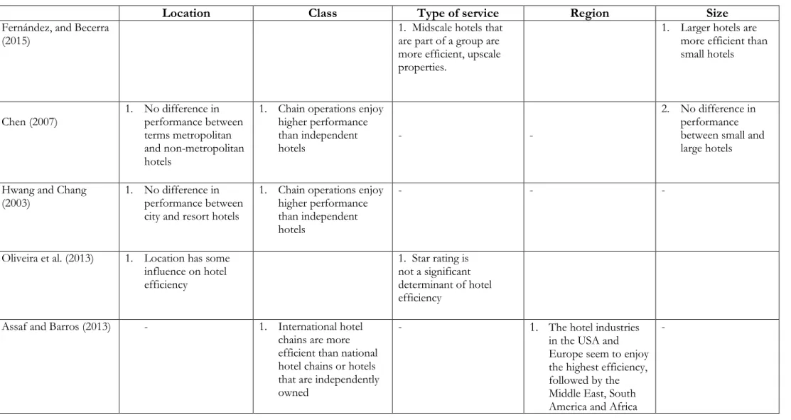
Location Class Type of service Region Size
Fernández, and Becerra
(2015) 1. Midscale hotels that are part of a group are more efficient, upscale properties.
1. Larger hotels are more efficient than small hotels
Chen (2007) 1. No difference in performance between terms metropolitan and non-metropolitan hotels
1. Chain operations enjoy higher performance than independent
hotels - -
2. No difference in performance between small and large hotels
Hwang and Chang
(2003) 1. No difference in performance between city and resort hotels
1. Chain operations enjoy higher performance than independent hotels
- - -
Oliveira et al. (2013) 1. Location has some influence on hotel efficiency 1. Star rating is not a significant determinant of hotel efficiency
Assaf and Barros (2013) - 1. International hotel chains are more efficient than national hotel chains or hotels that are independently owned
- 1. The hotel industries in the USA and Europe seem to enjoy the highest efficiency, followed by the Middle East, South America and Africa
Assaf (2012) - 1. International hotels have a slightly higher efficiency than local hotels.
- 2. Australia, Singapore and South Korea have the most efficient hotel industry in the Asia Pacific region.
-
Wang et al. (2006) 1. Hotel located in metropolitan areas enjoy higher performance than those in other areas
1. Chain operations enjoy higher performance than independent hotels
- - -
Yu and Lee (2009) 1. Resort hotels enjoy higher performance than city hotels
1. Chain operations enjoy higher performance than independent hotels
- - 1. A U-shaped
relationship between size and hotel performance. The largest hotels demonstrated strong performance than smaller size hotels
Pulina et al. (2010) - - - - 1. Medium-sized
hotels demonstrated the strongest performance, followed by small hotels
Assaf and Knezevic
(2010) - - 1. Star rating is a significant
determinant of hotel efficiency - 1. Large hotels demonstrate stronger performance than small hotels Assaf and Agbola
(2011) 1. City hotels demonstrate stronger performance than - 1. Star rating is a significant determinant of hotel - 1. Large hotels demonstrate stronger
located elsewhere efficiency performance than small hotel. Aissa and Goaied
(2016)
1. Hotels with scenic and coastal location demonstrate stronger performance than hotels in other locations
1. Chain operations enjoy higher performance than independent hotels - - 1. Large hotels demonstrate lower profitability performance than small hotels
3. The Model
Our point of departure is to model heterogeneity in a flexible way and then measure productivity and efficiency. The classical approach, without heterogeneity, rests upon the following specification:
y
it
x
it
v i
it,
1,..., ,
n t
1,..., ,
T
(1) which is the classical linear model, wherex
it is a k1 vector of covariates, is a k1 vector of parameters, andv
it is an error term.Here, we propose a model to account for heterogeneity. Known alternatives are the finite mixture model (which has been made more flexible in Geweke and Keane, 2006) and the random coefficient approach (Tsionas, 2002). Here, we opt for a more flexible approach, which allows environmental variables to influence directly the heterogeneity (called, for this reason, observed heterogeneity).
Our model is:
y
it
x
it
z
it
v i
it,
1,..., ,
n t
1,..., ,
T
(2)where
z
it is p1 vector of environmental variables (size, classification, etc.). Here, ℝd will denote, thereafter, the parameter vector. Hence in our formulation we make depend onit
z
.2 Here, is also random itself and has also random error term that it different by hotel. We elaborate further on this formulation in more detail below.Moreover, we modify the model in (2) as follows:
,
1,..., ,
1,..., ,
it it it it it it
y
x
z
v
u i
n t
T
(3)where a common specification is:
2
~ 0, ,
it u
u N (4)
and uit0 is an error component that stands for technical inefficiency
3. The specification in (4) is highly restrictive, mainly for two reasons. First, it does not allow an examination of how environmental variables affect inefficiency. Secondly, and perhaps more importantly, it does not allow an examination of how inefficiency and productivity growth are interrelated. This is, indeed, an open question, for the most part. For example, we know that productivity growth is
2 This is known as a smooth coefficients model in the literature. See for example Li at al (2002) . 3 We have +
it
u
in the case of cost functions and –u
it in the case of production functions. This corresponds also, respectively, to output distance functions and input distance functions.technical change plus efficiency change suggesting that productivity growth depends on (a) shifts of the frontier, and (b) movement inside the frontier (movement that hopefully leads to better input – output combinations). From the “growth accounting” point of view this is fine but it does not address an examination of two interesting questions: (i) Does higher efficiency lead to shifts of the frontier? (ii) Do shifts in the frontier also imply improvements in efficiency practices? Regarding (i) one may argue that better management practices often lead to adoption of better technologies as well. Regarding (ii) one may argue that adopting better technologies is also evidence of more efficient use of resources in the context of the new technology. Of course, the answer to these questions ultimately lies in the data but we need an appropriate model to relate both efficiency and productivity together. This paper aims to achieve this.
To illustrate, we add here to the model in (3)
it to account for unobserved productivity, and the distributional properties of the two-sided error termv
it,1 will be presented in what follows. Tomeasure productivity we assume a model similar to Levinsohn and Petrin (2003):
it
10
11 i t, 1
12log
u
i t, 1
z
it
1
it,1 (5)The difference from Levinshohn and Petrin (2003) is that productivity depends on inefficiency and other variables in the vector zit . In addition productivity is persistent through the parameter
21
.Finally, regarding
u
it we assume:(6)
Notice that in this model, inefficiency and productivity are related through a vector autoregressive (VAR) scheme. While efficiency and productivity can affect each other, we have not seen this formulation adopted in previous studies. Our process is also dynamic which allows us to examine impulse responses from one variable to the others for different groups but also for different hotels. The advantage of the approach is that we can examine whether improvements in productivity also lead to better efficiency and vice versa, as we mentioned in the discussion above.
We also address two important issues:
i) We can take outputs as exogenous4 but inputs are endogenous. ii) For several inputs, we do not have input prices.
4 This assumption is realistic in the hotel industry in the sense that input distance functions are compatible with cost minimization which, in turn, is a reasonable and minimal assumption to make.
20 21 , 1 22 , 1 2 ,2
We will discuss how we handle “ii” later below and why (i) and (ii) are related. Here we address endogeneity in inputs by estimating a system of equations that couples the distance function with the first order condition of the cost minimization problem. To illustrate, suppose all feasible combinations of inputs K
X
ℝ
and outputs MY
ℝ
are described by the technology setT
. An input distance function D X Y( , )1 describes production opportunities. Its definition is:
1
1 , max : : , , D X Y X Y T (7)where
1 implies efficient production. The cost minimization problem is:
,
m in : , s.t.
,
1. K X C W Y W X D X Y ℝ (8)It is known that the first order conditions (FOC) have the form:
ln , ,1,..., , ln , k k k D X Y W X K X C W Y (9)see Färe and Primont (1995). If lower case letters denote logs then we can write the FOC as follows:
,
ln k k ln , 1,... . k D x y w x TC k K x (10)Since one share equation will be omitted:
1 1 , , ln ln k k , 2,... . k D x y D x y w x x k K x x ɶ (11) where 1 1ln
K, , 2,...,
k kW
w
w
w
k
K
w
ɶ
. Suppose we have panel data. If we use a translog functional form we can write the log distance function as follows:1 0 1 , 2 1 1 , , 1 , 1 , , , , ,1 2 1 1 1 1 , K K K M k k it kk k it k it m k k k m m it M M K M mm m it m it km k it m it it it it m m k m x x x y y y x y v u
(12) where i1,..., ,n t 1,...,T ,x
ɶ
k it,
x
k it,
x
1,it,
k
2,...,
K
.Using the homogeneity of degree one of the distance function in terms of inputs, we can impose the constraints: 1 1, 1 0. K K k kk k k
(13) Moreover,
, , 1 1 , , , 1,..., . K M it it k k kk k it m km m it k it D x y x y k K x
Therefore, after introducing random errors,
k it, , we can write the FOC as follows:, , 1 1 , , 1, , 1 1 1 , 1 1 , ln , 2,... . K M k k kk k it m km m it k it k it it it k K M k k it m m it k m x y w x x v k K x y
ɶ (14)Our complete model is, then, as follows: Distance function: 1 0 1 , 2 1 1 , , 1 , 1 , , , , ,1 2 1 1 1 1 , K K K M k k it kk k it k it m k k k m m it M M K M mm m it m it km k it m it it it it m m k m x x x y y y x y v u
(15) FOC: , , 1 1 , , 1, , 1 1 1 , 1 1 , ln , 2,... , K M k k kk k it m km m it k it k it it it k K M k k it m m it k m x y w x x v k K x y
ɶ (16)
,1,
,2,...,
,~
0,
it it it it K KV
v
v
v
N
The first order conditions provide a set of equations that determine the endogenous variables of the model. In this sense, the first order conditions can be used to account for endogeneity in an economically plausible manner.
Productivity: 10 11 , 1 12
log
, 1 1 ,1.
it i tu
i tz
it it
(17) Inefficiency 20 21 , 1 22 , 1 2 ,2log
u
it
i t
log
u
i t
z
it
it,
(18) ,1,
,2~
(0, ).
it it itN
Notice that the two errors terms in (17) and (18) are correlated.Flexible coefficients
To elaborate further on how we account for heterogeneity (the crux of the matter in this paper) suppose we collect all coefficients , , , into a vector
whose dimensionality is d1.Given the p1 vector of environmental variables
z
it the coefficients are made flexible through the following model:
1 1 2
3
, , 1,..., , G j zit ajo a zj it g aj z ait j j j d
(19) where
1 1 e is the logistic function also known as sigmoid. The model is an
artificial neural network (ANN) with G nodes and it is known that as G increases it can approximate accurately any functional form (see Hornik et al, 1989). A major innovative aspect of the model is that we introduce random terms
,j,
j
1,..., ,
d
in (19) for which we assume:,j,..., ,d ~Nd(0, ).
(20)
In the smooth coefficients literature the coefficients do not contain error terms and, therefore, most studies do not account for unobserved heterogeneity (observed heterogeneity is the part that is related to the environmental variables in zit). By introducing these errors we address the
issue of unobserved heterogeneity and the coefficients are also random. In (19) if aj10 and
2 0
j
a then the coefficients are purely random and there is no observed heterogeneity. If the variances of
, j are zero, then there is no unobserved heterogeneity and the coefficients are notrandomly varying.
Let us illustrate this construction in the simple linear model with one regressor:
y
z x
t t
v
t. Using an ANN for
z
t we have:
3 1 1 1 2
1
t G a z t o t g tz
a
a z
a
e
. Since thecoefficients follow an ANN they are flexible in the sense that they can approximate any functional form arbitrarily well as G increases. The choice of G is, of course, an empirical matter. Therefore, the final model is:
3 3 1 1 1 2 1 1 1 2 1 1 . t t G a z t o t g t t t G a z o t t t g t t t t y a a z a e x v a x a x z a x e v x
(21)The first feature of the model is that the effect of
x
t ony
t depends onz
t as it is evident from the following expression:
3
1 1 1 2(
| , )
1
t.
G a z t t t o t g t tE y x z
a
a z
a
e
z
x
(22)The effect is not monotonic and it is not necessary that it has the same sign for all z. The second feature of the model, is that we have conditional heteroskedasticity. Indeed, the error term
t t t t
e
v
x
has variance 2 2 2mentioned that since the coefficients are flexible functions of a set of variables, the final model is itself flexible, in the sense we defined, viz. Hornik et al (1989) and Hornik (1991).
Unobserved prices
As mentioned in “ii” one commonly encountered problem is that most if not all input prices are unobserved.5 For them we assume:
,
,
2,..., ,
1,..., ,
1,..., ,
k it k ki ktw
ɶ
k
K i
n t
T
(23)where
k,
ki,
kt are unknown parameters. Specifically,
ki is a random effect that represents variations of the kth input price across firms and
kt is a random effect that represents common temporal variation of the kth input price. Specifically,
2
~ , , 1,..., , 1,..., , ki N k K i n (24) where 2
is related to the degree of competition in the market ( 20
means that all hotels are price takers). Moreover
2
~ , k k N k , where 2 20,
10
k k
. Additionally, , 1,
2,..., ,
1,..., ,
kt k k t ktk
K t
T
that is, log relative prices follow an AR(1) process. We treat
k0as unknown with a prior:
0
2 0~ 0, k k N k where 20 00,
k1
k
. For
k we assume k ~ N
k,2k
, where2 1
2
,
k1
k
. For the
kts we assume:
,
2,...,
~
1
0,
.
t kt
k
K
N
K
Before proceeding it is, perhaps, worthwhile to mention that the introduction of a model of prices in the FOCs is a general way of introducing individual and time – related effects in the distance function – FOC system. The general approach of making distance function intercepts vary by individual a la fixed – effects, is somewhat arbitrary in the sense that it does not necessarily exhaust all available heterogeneity and, perhaps more importantly, it does not reflect differences in managerial practice (which are captured by uit in any case). Some attempts have
been made in the literature to assume that all coefficients in a translog function are random but these coefficients lack structural interpretation and, therefore, it is not clear what is accomplished in this modeling context.
To proceed, we have to recognize that the distance function and the FOCs form a simultaneous equations system. To accounting for simultaneity we have to derive the Jacobian of transformation from the error terms to the endogenous variables. To derive the Jacobian define the following expressions for simplicity:
, , , 1 1 , 1,..., , K M k it k k kk k it m km m it D
x
y k K (25) , , 1 1 , 1 1 1 , 1 1 , , 1,..., , K M k k kk k it m km m it k it K M k k it m m it k m x y r k K x y
1, 1 , , 2 , , 1, , , 1,..., , kk it k k it kk it kk kk it kk k it it D D G G k k K r D
ɶwhere
kkdenotes Kronecker’s delta (
kk
1
if kk and zero otherwise). Define also: 1,,...,
,,
itD
itD
K it
d
, , , 1,..., 1. it Gkk it k k KIK GThen, the Jacobian of transformation of the system of distance function and FOC is the following:
det , it it J A (26) where it it it d A G .We provide statistical inferences of the model using efficient Markov chain Mote Carlo (MCMC) procedures for Bayesian analysis. As mentioned above, MCMC is needed because the likelihood function depends on multivariate integrals that are not available in closed form. The multivariate integrals are with respect to the latent prices, latent productivity and inefficiency and the error terms in the flexible coefficients β(zit). We provide in Appendix 1 more technical details about the model and the Bayesian inference procedures.
4. Data and Variables
The dataset for this study was obtained from Smith Travel Research, an independent company that tracks lodging supply and demand data for most major hotels in the US and internationally.
The STR’s data are highly comprehensive, reliable and mostly commonly by hotels to track their performance6.
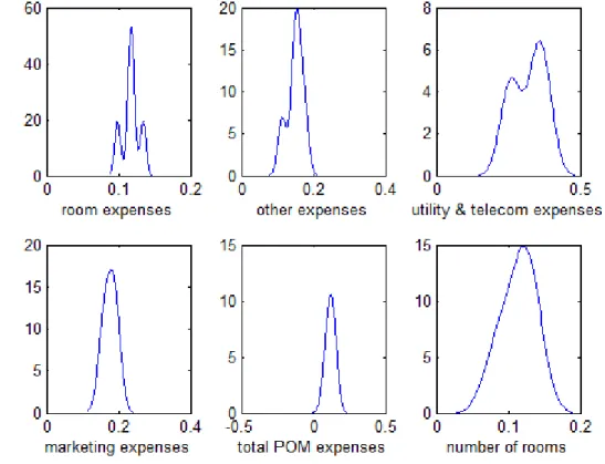
We use here a unique panel sample of 613 hotels (for the years 2012-2016) located across the US, Europe, Middle East and the Asia Pacific (613*5 years=3065 observations). The data cover a rich list of inputs, outputs and environmental variables. For outputs we use total room revenues, total other revenues (food and beverage revenue, telecommunication revenue, other operational revenue and miscellaneous income), and occupancy rate. For inputs, we use total room expenses, total other expenses (food and beverage expenses, other department expenses, and administrative and general expenses) total utility and communication expenses, total marketing expenses, total property and maintenance (POM) expenses, and number of rooms available. While most of these variables have been used in related studies in the literature (e.g. Salman Saleh et al. 2012; Barros, 2006; Barros and Santos, 2006 and Assaf and Agbola, 2011), it is rare to see a study combining them all in one model. With such a detailed breakdown of inputs and outputs, our aim is to 1-provide a more comprehensive assessment of hotel performance, and 2-assess the contribution of each of these inputs and outputs toward hotel performance. Table 3 provides some descriptive statistics of these variables. In Figure 1, we provide the average derivatives of the distance function with respect to the variables indicated to ensure that we have the monotonicity properties in place.
For the environmental variables “zit ” (see equation 2), we account for the following
characteristics:
1- Location (urban, airport, suburban, interstate, small metro/town and resort) 2- Type of service (Full service vs. limited service)
3- Size (small hotels vs. large hotels)7
4- Region (US, Asia Pacific, Europe and the Middle East)
5- Class (luxury chain, upper upscale chain, upscale chain, upper midscale chain, midscale chain, economy chain, and independent).
All these variables are measured as dummies using the same classifications adapted worldwide by Smith Travel Research. For example, STR classifies (e.g. luxury chain, upper upscale chain, etc.) hotels based on the average daily rate (ADR). STR defines a limited Service hotel as a “property that offers limited facilities and amenities, typically without a full-service restaurant”, while full- service hotels “usually offer a wide variety of onsite amenities, such as restaurants, meeting spaces, exercise rooms or spas”.
6 At least in the United States.
7
In this study, we follow Shang et al (2008) and classify hotels into two main categories, namely, small as those with less than 300 rooms, and large hotels as those with more than 300 rooms.
Table 3. Descriptive Statistics of Input/Output Variables
Variable Observations Mean Std. Dev. Min Max
Total Room Revenue 3,065 9708205 1.74E+07 655336 2.25E+08
Total Other revenue 3,065 4846354 1.11E+07 1299 1.20E+08
Occupancy 3,065 72.6 10.16191 30.6 98.2
Total Room Expenses 3,065 2512993 5267745 125528 6.39E+07
Total Other Expenses 3,065 4369014 9451974 39693 1.17E+08
Total Utility and Telecom
Expenses 3,065 654637.3 1091965 44093 1.38E+07
Total Marketing Expenses 3,065 997672.1 1631646 36281 1.99E+07
Total POM Expenses 3,065 622933 1122650 33913 1.34E+07
Number of Rooms
Available 3,065 81439.73 78011.65 14600 725039
5. Results
5.1. Sensitivity Analysis, Convergence, and Model Comparison
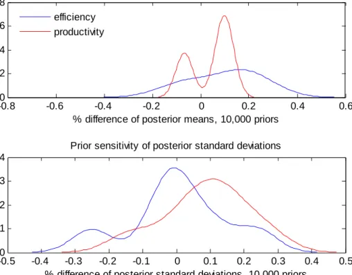
As the Bayesian approach can be sensitive to the choice of “prior”, we first examined the sensitivity of our efficiency and productivity result to various prior choices. Specifically, we generated 10,000 random prior parameters and we applied the sampling-importance-resampling (SIR) approach of Rubin (1987) to compute the new posterior means and standard deviations of the parameters and the new posterior means and standard deviations of efficiency and productivity. The 10,000 differences relative to baseline posterior means and standard deviations are reported in Figure 2 below.
Figure 2. Prior Sensitivity of Posterior Mean and Posterior Standard Deviations
Next, for each efficiency and productivity distribution for the 10,000 priors we use the Anderson and Darling test to test for equality of distributions. The p-values of the test across all priors are reported in Figure 2. The p-values average 0.17 and range from 0.10 to 0.26 showing that the null of equal distributions cannot be rejected. These results indicate that prior sensitivity is not an important issue in this study so we can proceed with reporting results from our baseline prior specification. -0.80 -0.6 -0.4 -0.2 0 0.2 0.4 0.6 2 4 6 8
% difference of posterior means, 10,000 priors
d e n s it y
Prior sensitivity of posterior mean efficiency productivity -0.50 -0.4 -0.3 -0.2 -0.1 0 0.1 0.2 0.3 0.4 0.5 1 2 3 4
% difference of posterior standard deviations, 10,000 priors
d e n s it y
Figure 3. P-value of the Anderson-Darling Test
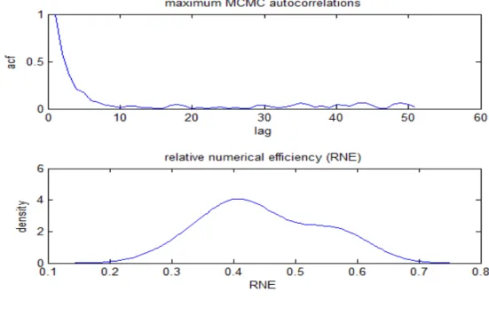
To assess convergence of the of the MCMC chain, we also monitored the relative numerical efficiency (RNE) and the MCMC correlations. From MCMC autocorrelations8 we see that the first few ones are small and quickly drop to zero indicating successful convergence. If this pattern does not occur, then the posterior is not thoroughly explored and we may need to take thousands or even millions of additional MCMC iterations. The Relative Numerical Efficiency (RNE) (see Geweke, 1992), is another assessment of convergence and is usually used to measure how close to independently and identically (IID) distributed sample we are, where a value of 1 indicates that we have, effectively, IID sampling from the posterior, while a value of zero indicates poor performance of MCMC. As we can see from the RNE distribution, the average RNE is close to 0.5, which indicates relatively good performance.
Figure 4. MCMC Autocorrelations and RNE
8 We report maximum autocorrrelations taken across all parameter draws as well as draws for all latent variables in the model.
0.080 0.1 0.12 0.14 0.16 0.18 0.2 0.22 0.24 0.26 2 4 6 8 10 12 14 16 18
p-value of Anderson-Darling test
d e n s it y
Anderson-Darling test of equality of distributions with baseline posterior inefficiency productivity
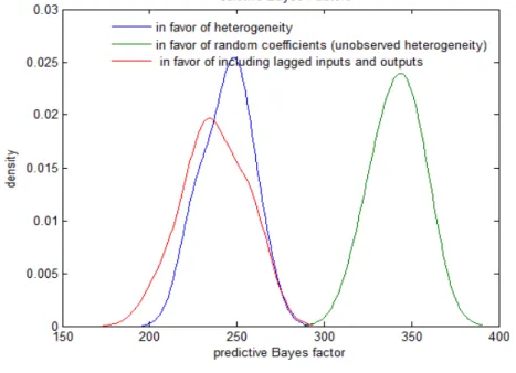
Having confirmed that inferences are robust to the prior and MCMC performs well, we proceed to test different modelling specifications using the predictive Bayes factor (a predictive Bayes factor>1 indicates support for the “null” model)9, where the base for each case is a model that does not include the desired specification (i.e. no heterogeneity, no random coefficients and no lagged inputs and outputs) highlighted in Figure 5.10 Note that “in favour of random coefficients” means whether error terms
, j are zero. “In favour of heterogeneity” means β(z)does not depend on z. It is clear from Figure 5 that accounting for heterogeneity is supported by the data. There is also clear support for including the lagged values of inputs and outputs, which controlled for in our estimation.
Figure 5. Predictive Bayes Factor of Various Competing Models
9 To implement the computation of predictive Bayes factors we omit 10 randomly selected observations from the sample at a time and we repeat this 1,000 times to obtain the distributions shown in Figure 5. For a model with data Y and “future data” Y’ the predictive density is p(Y’|Y) which can be obtained from p(Y’,θ|Y) by integrating out the parameters θ. This involves the following computation: ∫P(Y’,θ|Y)dθ=∫P(Y’|θ,Y)p(θ|Y)dθ, where p(θ|Y) is the posterior distribution. For two models, say 1 and 2, the predictive Bayes factor is p1(Y’|Y)/p2(Y’|Y). This integral is, in most interesting cases, not available analytically. The parameters need not be the same for the two models. Higher values for the predictive Bayes factor is p1(Y’|Y)/p2(Y’|Y). The parameters need not be the same for the two models. Higher values for the predictive Bayes factor indicate preference for model 1 in terms of out-of-sample predictive ability.
5.2. Efficiency and Productivity Growth
Hence, the above provides direct confirmation of the importance of accounting for heterogeneity when analysing the performance of the hotel industry, and illustrate the importance of differentiating hotels based on the various environmental variables we discussed in section 4. The efficiency and productivity growth results (based on our baseline priors) are presented in Figures 6 and 7. In Tables 4 & 5, we also present the average efficiency and productivity growth for each hotel classification, along with the posterior standard deviation11. Finally, in Figures 8 and 9, we discuss how the various inputs and outputs in our sample contribute to efficiency and productivity growth.
We observe the following:
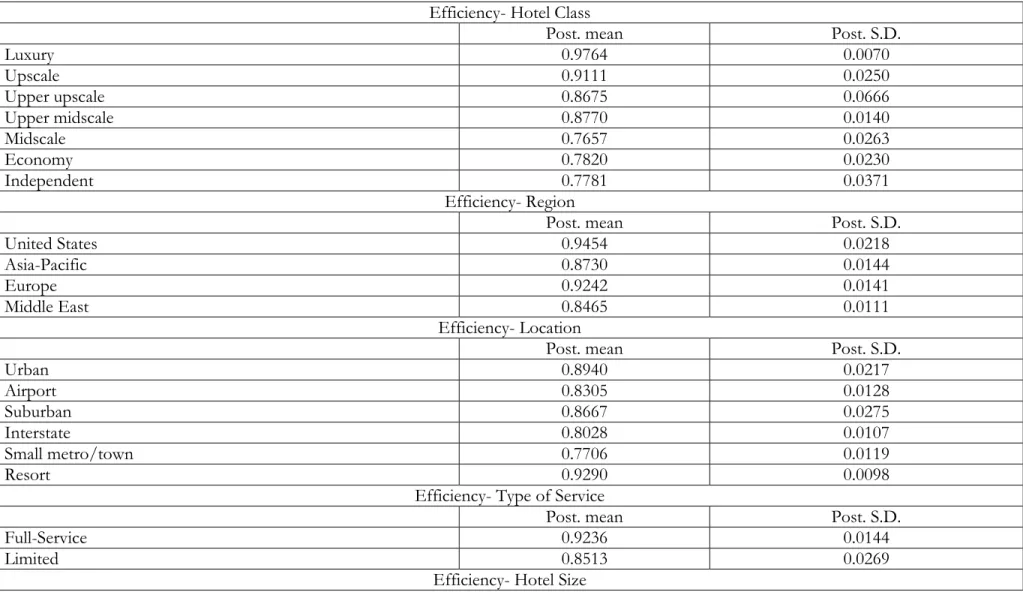
1- First, it is clear from the efficiency distributions in Figure 6a, as well as the first part of Table 4, that luxury hotels have outperformed all other hotel classes. They are operating at an average efficiency of 97.64% (i.e. only 2.36% away from achieving maximum efficiency). The second best performing group include the upper upscale, upscale, and upper midscale chain hotels, which do not seem to perform significantly better than each other. The worst performing group include the midscale, economy and independent hotels.
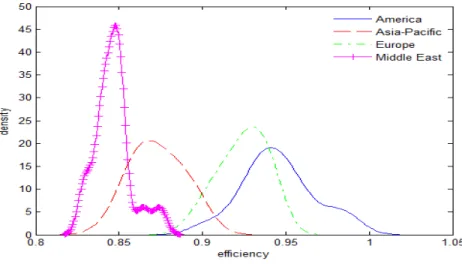
2- Second, from Figure 6b, and the second part of Table 4 we can see that hotel industries in the United States and Europe seem to enjoy the highest efficiency. The United States, in particular, has the highest efficiency in the sample with an average of 94.54%. The Asia-Pacific region has the third highest efficiency, though this is not significantly different from the Middle East in fourth.
3- Third, from Figure 6c, and the third part of Table 4, it is clear that resort, urban and suburban hotels seem to enjoy the highest efficiency. Resort hotels, in particular, have the highest efficiency in the sample with an average of 92.90%. This group seems also to be performing significantly better than the second best performing group, which includes airport, interstate, and small/metro town hotels. The lowest efficiency belongs to hotels located in small/metro town with an average of 77.06%.
4- Fourth, from Figure 6d and Table 4 it is clear that full-service hotels have significantly higher efficiency (92.36%) than limited-service hotels (85.13%). This goes in line with our finding in (1), because full service hotels usually include upscale, upper upscale and Luxury properties and offer a wide range of services such as restaurants, meeting spaces, exercise rooms or spas.
5- Fifth, from Figure 6e and the last part of Table 4, we can see that large hotels do not necessarily enjoy higher efficiency than small hotels. The difference between the two is marginal and not statistically significant.
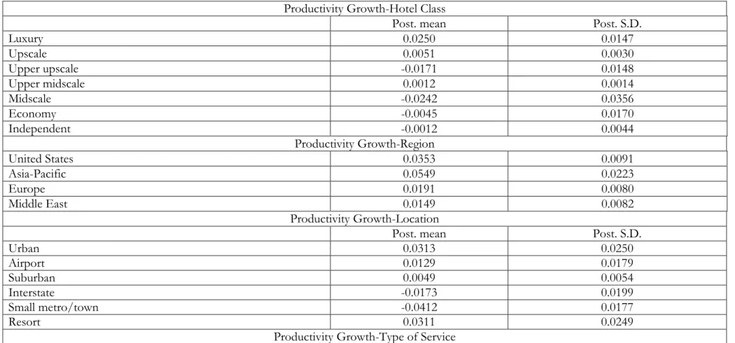
6- Sixth, from the various productivity growth distribution figures (figure 7a-7e) and Table 5, it is clear that productivity growth does not necessarily experience the same behaviour as efficiency. In general, there is no compelling prior reason why this would should be
11 If the densities in figures 6 and 7 overlap, this is a clear indication that the difference in efficiency or productivity is not significant.
the case. For instance, in most cases, the productivity growth rate is small and statistically insignificant. To illustrate, luxury hotels, which rank first, have only experienced a productivity growth of 2.5 %, while economy and independent hotels have experienced a negative productivity growth. In terms of regional difference, the Asia-Pacific and the US have experienced the highest productivity growth (5.49% and 3.53%, respectively), followed by Europe and the Middle East. We did not notice significant differences in terms of productivity growth by location. Urban hotels have experienced the highest productivity growth (3.13%) while small/metro town hotels have experienced the highest productivity decline (-4.12%). Similar to our efficiency results, we did not find significant difference in productivity between small and large hotels. Full-service hotels, on the other hand seem to be performing slightly better in terms of productivity growth (1.32%) than limited-service hotels (-2.36%).
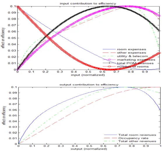
7- Seventh, we assess how the various inputs and outputs affect efficiency and productivity growth. As discussed above, productivity and efficiency have also parameters, which depend on “zit”. Therefore, input and output contributions toward productivity and
efficiency can be computed easily using partial derivatives of (17) and (18) using (19), as in (22) with respect to inputs and outputs. The results are presented in Figures 8 and 9. We can see (Figure 8) that inputs do not generally have a linear relationship with efficiency, but investments of inputs such as marketing and maintenance seem to lead to an increase in efficiency. The story is however different for the number of rooms, room expenses and other expenses where the gain in efficiency seems to become marginal as these inputs increase. This goes in line with our previous finding that an increase in the size of hotels (i.e. number of rooms) does not necessarily result in higher efficiency. From the output results, we see that increase in outputs result generally in higher efficiency. The highest gain (on average) comes from “room revenues”, though this gain does not seem to be significantly higher than other outputs. The relationship with productivity is also highly similar to the efficiency context (Figure 9). For instance, it is clear that the gain in productivity growth becomes marginal as the number rooms, room expenses and other expenses increase, while on the outputs side, an increase in occupancy rate and room revenue seems to result in the highest gain in productivity growth. We provide more reflection on these findings below.
5.3. INTERRELATED PRODUCTIVITY AND EFFICIENCY
We discussed that it is possible to expect a relationship between productivity and efficiency that goes beyond the traditional growth accounting convention that productivity growth equals technical change plus efficiency change. Indeed, this is the crux of the matter in a dynamic formulation like (17) – (18). Since the γ and ρ coefficients in (17) and (18) are flexible functions of the environmental variables in zit, the specification is quite flexible. As the zits also appear in a linear manner in the specification of the flexible coefficients in (2) and (19), we can assume without loss of generality that γ1=γ2=0. There are two interesting questions that we can address. (i) Is there persistency in productivity and inefficiency? If not then we expect ρ11=ρ22=0. (ii) Is there any interrelatedness between productivity and inefficiency? If not we should expect ρ12=ρ21=0.
The ρ coefficients (like all other ‘structural’ parameters in our model) are flexible functions of zit so an examination of these questions is not trivial and depends on the specific values of these environmental variables. Given MCMC draws for the ANN parameters in (19) these coefficients can be evaluated and we can present their posterior means at selected values of the zits. The results are shown in Table 5.
Most persistence coefficients (ρ11 and ρ22) are away from zero. This is reasonable as we expect some persistence in both inefficiency and productivity. Both shocks in production (productivity) as well as managerial practices (related to inefficiency) are, usually, persistent. The effect of productivity on inefficiency (ρ21) is, generally, negative suggesting that more productivity growth, generally, contributes to lower inefficiency (higher efficiency). In this sense, upward shifts of the frontier, generally, contribute to better utilization of resources as well, and the resulting input – output mix is closer to the new frontier. In most cases there is a negative effect of inefficiency on productivity (ρ12<0). In these cases, inefficient hotels are also less productive. In certain cases the coefficient is practically zero, so that there is no effect, yet in others it is positive. In this case, we can argue that less efficient hotels adopt practices and re-arrangements to become more productive as their distinction between efficiency and productivity is not clear. We find that this is the case for hotels that are not large, luxury, upscale or midscale or located in urban areas or resort hotels. For such hotels, it is possible that inefficiency acts as a “buffer” and enjoy what is known as “quiet life”: Provided they do acceptably well, they do not want to sacrifice real resources to decrease inefficiency but when it becomes inevitable, they prefer to adopt new technologies to increase productivity growth. The subject clearly requires some investigation in future research in the context of tourism, although the “quiet life hypothesis” has received considerable attention in banking studies (Koetter at al., 2012).
6. Discussions
Our aim with the use of a large sample coupled with the adoption of a more advanced methodology was to provide a more robust assessment of hotel performance and untangle some of the contradictions in the literature. For the first time, we assessed the impact of size on two performance metrics: efficiency and productivity growth. Importantly, we also accounted for heterogeneity in doing so. Most studies assume that production technologies are similar. However, as Pack (1982) stated, technology differences are highly essential when comparing firms of differing size.
From our results, we did not conclude that size is negatively correlated with either efficiency or productivity growth, contradicting the findings of several other studies in the area, while supporting others (Table 2). In other words, being large does not seem to really matter in the hotel industry, a finding that can be of interest to both academicians and hotel practitioners. The finding can also incentivize large hotels to pay more attention to alternative efficiency improvement strategies. Within the broader business literature, studies did not also confirm that size necessarily affects performance (Page, 1984; Diaz and Sánchez, 2008; Aggrey et al. 2010). It is usually claimed that larger firms can “be more efficient in production, because they could use more specialized inputs, coordinate their resources better, enjoy the advantage of scale
economies, etc.”, but there is also the counterargument that these firms have less incentive to improve efficiency because of their market power (Yang and Chen, 2009, p.378). One can also make the argument that small firms are “exposed to more competition than larger firms are and respond quickly to outside change. Therefore, in the test of a changing environment, perhaps small business prove to be the fittest form of an organization” (Yang and Chen, 2009, p.378). While size did not show to be an important factor, our results provided further supporting and reassuring evidence that location, type of service (full vs. limited), and class are all important matters when it comes to hotel performance. Specifically, we found that resort, urban and suburban hotels seem to enjoy significantly higher efficiency than hotels located in airport, interstate and small/metro town locations. Such findings are line with Chen (2007) and Hwang and Chang (2003), though none of the previous studies has differentiated or compared between these six different locations12. It was also interesting to see that full-service hotels perform significant better on efficiency than limited-service hotels, as this might create an incentive for the latter group to improve their services or offer new onsite amenities, such as restaurants, meeting spaces, exercise rooms or spas. Finally, the results clearly indicate that hotels located in the US have outperformed other locations. Such finding might be of interest not only for new investors, but also for hotels comparing their brands across various geographic locations.
The productivity results were not completely unexpected. As mentioned, productivity growth is not driven by efficiency alone, but also by technical change (i.e. innovation) and efficiency change rather than efficiency itself. In the hospitality industry, we all know that “we lag behind many others in introducing innovations to streamline our operations and run more efficiently” (Inge, 2014, p.38). In a recent study, Bilgihan et al. (2015. p. 203) further highlighted that “innovation is still a buzzword for many hotels, and the hospitality and tourism industries have been slow in adopting new technologies. The cost of innovation, resistance from owners, resistance to change, training issues, pace of advances in new technology, time, and budget constraints are some of the other barriers”. Companies such as Marriott have been investing more heavily in innovative technologies, launching recently programs such as TestBed, which give tech start-ups an opportunity to test their products within a Marriott facility. However, many other hotel companies are still reluctant to invest more in technologies. There is actually still a wide gap between hotels and companies in other industries such as retail and manufacturing (Marr, 2016). Hence, our results seem to be in line with the industry trends and may provide hotel operators with further validation that productivity growth is still a problem in the industry and may require further attention. Moreover, the adoption of new technology as a means to productivity growth has its limits: Once more hotels adopt the same new technologies the gains tend to disappear. The same happened for example to commercial banks with the introduction of ATMs. The first banks that introduced the technology experienced productivity growth, followed by the other banks, but once the stage has been set and the ATMs dominated the market, productivity edges and gains disappeared.
The study also shed light on how the various inputs and outputs contribute to efficiency and productivity growth. It was interesting to see how an increase in the number of rooms and room
expenses results only in marginal efficiency and productivity growth, while on the other hand an increase in room revenue does not necessarily result in higher performance gain than other outputs. Hence, the implication here is that hotels may need to develop appropriate strategies to increase room revenue without simply adding more rooms to their property. The largest hotels in our sample, for instance, did not necessarily have the largest room revenue. Such finding reinforces the importance of developing packages and bundles that add value to the consumer without creating too much cost for hotels (Kimes and Anderson, 2011). As other revenues (e.g. food and beverage revenue and miscellaneous income) have also equal contribution to efficiency and productivity growth, hotels may also consider further investments in these areas. It is true that “while some of these facilities (most notably, food and beverage) have lower profit margins than rooms, they can still provide additional cash, which can help sustain your hotel during low-demand periods “(Kimes and Anderson, 2011, p. 405).
Finally, the study also analysed the persistence level of inefficiency and productivity. We showed that both shocks in inefficiency and productivity are usually persistent. In other words, hotels are expected to operate with a relatively high level of inefficiency over time unless some adjustments in policy and/or management take place. Hence, hotels cannot expect inefficiency or low productivity to correct themselves. They need rather to have effective strategies in place to ensure the effect of shocks do no persist over time (One example of shock can be a high probability that a competitor may dominate the market) (Comin, 2010). Importantly, we also showed that inefficiency and productivity are generally related. Hence, hotels cannot look at the two separately, or ignore one and focus on the other. This has important implication, as hotels should not focus their investments in one of these areas. They might be actually wasting resources by investing in inefficiency and ignoring productivity, or vice versa.
7. Concluding Remarks
This paper developed a new Bayesian stochastic frontier model that accounts for heterogeneity in a highly flexible way and that can measure both efficiency and productivity, simultaneously. The model addressed the endogeneity problem in inputs using the first order conditions from an input distance function and cost minimization. The use of first order conditions takes care of the endogeneity problem by adding the missing equations for the endogenous variables of the model. Unfortunately, prices are often missing and this approach is hard to implement. However, we controlled for the issue of unobserved prices by assuming that relative prices are latent and can be related to input-specific and time-specific effects. The model can be simply extended to other tourism applications. The model, for instance, is highly appropriate to assess the efficiency of tourism destinations as it can account for the heterogeneity between different tourism destinations.
We used a unique and rich sample covering 613 hotels located across the US, Europe, Middle East and the Asia Pacific13. We provided estimates of efficiency and productivity growth and assessed how these measures vary by location, hotel class, type of service, region and size. With
such large sample, we provided further validation to the impact of these determinants on hotel performance. We showed that large hotels do not necessarily perform better than small hotels. We also showed that hotel efficiency differs based on location, geographical region and type of service. The results further indicated that productivity growth is still not a driving force in the industry. We also discussed how various inputs and outputs contribute to efficiency and productivity growth. In particular, we find very little productivity growth with the new model, suggesting that the introduction of new technologies has exhausted its potential and managers need to find other ways to increase productivity. Finally, we discussed the persistence of shocks in inefficiency and productivity and illustrated how inefficiency and productivity are strongly interrelated.
While our results have important implications to both academicians and hotel practitioners, they are not without limitations. We believe that other hotel characteristics (e.g. service quality, star rating, etc.) may also affect efficiency and productivity growth, but accounting for these variables was not possible due to data limitation. We also believe that future studies may consider validating the results with some on-site case studies of some individual hotels. This may provide a better reflection on the strategies adopted at these sites and may better explain the nature of some of our findings.
On the other hand, our smooth-coefficient approach with unobserved heterogeneity may account implicitly for quality differences through the use of characteristics (zit) that are correlated with quality. Therefore, it is not altogether true that quality considerations are entirely missing from our analysis.
Fig. 6a. Efficiency distributions based on hotel class Fig. 6b. Efficiency distributions based on region
Fig. 6c. Efficiency distributions based on location Fig. 6d. . Efficiency distributions based on the type of service
Fig.7. Productivity distributions based on hotel class Fig. 7b. Productivity distributions based on region
Fig. 7c. Productivity distributions based on location Fig. 7d. Productivity distributions based on the type of service Figure 7. Productivity Growth Analysis by Various Hotel Characteristics
Table 4. Efficiency Analysis
Efficiency- Hotel Class
Post. mean Post. S.D.
Luxury 0.9764 0.0070 Upscale 0.9111 0.0250 Upper upscale 0.8675 0.0666 Upper midscale 0.8770 0.0140 Midscale 0.7657 0.0263 Economy 0.7820 0.0230 Independent 0.7781 0.0371 Efficiency- Region
Post. mean Post. S.D.
United States 0.9454 0.0218
Asia-Pacific 0.8730 0.0144
Europe 0.9242 0.0141
Middle East 0.8465 0.0111
Efficiency- Location
Post. mean Post. S.D.
Urban 0.8940 0.0217 Airport 0.8305 0.0128 Suburban 0.8667 0.0275 Interstate 0.8028 0.0107 Small metro/town 0.7706 0.0119 Resort 0.9290 0.0098
Efficiency- Type of Service
Post. mean Post. S.D.
Full-Service 0.9236 0.0144
Limited 0.8513 0.0269
Post. mean Post. S.D.
Large 0.9175 0.0114
Small 0.9231 0.0157
Table 5. Productivity Growth Analysis
Productivity Growth-Hotel Class
Post. mean Post. S.D.
Luxury 0.0250 0.0147 Upscale 0.0051 0.0030 Upper upscale -0.0171 0.0148 Upper midscale 0.0012 0.0014 Midscale -0.0242 0.0356 Economy -0.0045 0.0170 Independent -0.0012 0.0044 Productivity Growth-Region United States 0.0353 0.0091 Asia-Pacific 0.0549 0.0223 Europe 0.0191 0.0080 Middle East 0.0149 0.0082 Productivity Growth-Location
Post. mean Post. S.D.
Urban 0.0313 0.0250 Airport 0.0129 0.0179 Suburban 0.0049 0.0054 Interstate -0.0173 0.0199 Small metro/town -0.0412 0.0177 Resort 0.0311 0.0249
Post. mean Post. S.D.
Full 0.0132 0.0052
Limited -0.0236 0.0303
Productivity Growth-Hotel Size
Post. mean Post. S.D.
Large 0.0108 0.0067
Figure 8. Input and Output Contribution- Efficiency
36 Table 5. INTERRELATED PRODUCTIVITY AND EFFICIENCY
persistence interrelatedness 11 22 12 21 Luxury 0.312 (0.044) 0.617 (0.032) -0.027 (0.003) -0.045 (0.012) Upscale 0.289 (0.017) 0.718 (0.044) -0.032 (0.001) -0.052 (0.014) Upper upscale 0.216 (0.013) 0.515 (0.033) -0.045 (0.014) -0.059 (0.017) Upper midscale 0.117 (0.055) 0.782 (0.051) -0.051 (0.007) -0.032 (0.006) Midscale 0.128 (0.035) 0.812 (0.033) 0.032 (0.028) 0.017 (0.012) Economy 0.045 (0.032) 0.853 (0.041) -0.015 (0.022) -0.023 (0.019) Independent 0.032 (0.025) 0.891 (0.014) 0.013 (0.012) 0.030 (0.025) Urban 0.712 (0.023) 0.821 (0.017) -0.313 (0.018) -0.032 (0.002) Airport 0.789 (0.015) 0.815 (0.022) -0.276 (0.015) -0.017 (0.003) Suburban 0.414 (0.232) 0.314 (0.017) 0.122 (0.089) 0.020 (0.015) Interstate 0.280 (0.166) 0.288 (0.177) 0.103 (0.071) -0.144 (0.082) Small metro/town 0.171 (0.092) 0.119 (0.077) -0.215 (0.031) -0.071 (0.044) Resort 0.516 (0.025) 0.771 (0.014) -0.280 (0.045) 0.035 (0.021) America 0.642 (0.013) 0.717 (0.032) -0.122 (0.006) -0.045 (0.017) Asia-Pacific 0.315 (0.071) 0.689 (0.014) -0.035 (0.012) 0.032 (0.025) Europe 0.571 (0.014) 0.713 (0.025) -0.043 (0.007) -0.027 (0.009) Middle East 0.360 (0.120) 0.818 (0.045) 0.051 (0.017) 0.016 (0.012) Full 0.665 (0.022) 0.771 (0.022) -0.032 (0.004) -0.037 (0.007) Limited 0.215 (0.132) 0.891 (0.010) 0.012 (0.014) 0.011 (0.008) Large 0.412 (0.033) 0.680 (0.036) -0.045 (0.005) -0.032 (0.005) Small 0.881 (0.010) 0.881 (0.015) 0.033 (0.019) 0.017 (0.004)
37
References
Aggrey, N., Eliab, L., & Joseph, S. (2010). Firm size and technical efficiency in East African manufacturing firms. Current research journal of Economic theory, 2(2), 69-75.
Aissa, S. B., & Goaied, M. (2016). Determinants of Tunisian hotel profitability: The role of managerial efficiency. Tourism Management, 52, 478-487.
Anderson, R. I., M. Fish, Y. Xia, and F. Michello. (1999). “Measuring Efficiency in the Hotel Industry: A Stochastic Frontier Approach.” International Journal of Hospitality Management, 18 (1): 45-57.
Arbelo, A., Pérez-Gómez, P., & Arbelo-Pérez, M. (2017). Cost efficiency and its determinants in the hotel industry. Tourism Economics, 23(5), 1056-1068.
Ashrafi, A., Seow, H. V., Lee, L. S., & Lee, C. G. (2013). The efficiency of the hotel industry in Singapore. Tourism Management, 37, 31-34.
Assaf, A. G. (2012). Benchmarking the Asia Pacific tourism in