Internet banking: an exploration in technology diffusion and impact

(1)

Internet Banking: An Exploration in Technology

Diffusion and Impact

Richard Sullivan; Zhu Wang*

Payments System Research Department Federal Reserve Bank of Kansas City

Working Paper 05-05

November 25, 2005

Abstract

This paper studies endogenous diffusion and impact of a cost-saving technological innovation -- Internet Banking. When the innovation is initially introduced, large banks have an advantage to adopt it first and enjoy further growth of size. Over time, as the innovation diffuses into smaller banks, the aggregate bank size distribution increases stochastically towards a new steady state. Applying the theory to a panel study of Internet Banking diffusion across 50 US states, we examine the technological, economic and institutional factors governing the process. The empirical findings allow us to disentangle the interrelationship between Internet Banking adoption and growth of average bank size, and explain the variation of diffusion rates across geographic regions.

Keywords: Technology Diffusion, Bank Size Distribution, Internet Banking JEL Classification: G20, L10, O30

---

* Payments System Research Department, Federal Reserve Bank of Kansas City, 925 Grand Blvd., MO, 64198. Emails: [email protected]; [email protected]. We thank seminar participants at Fed Kansas City for helpful comments, and Nathan Halmrast for valuable research assistance. The views expressed herein are solely those of the authors and do not necessarily reflect the views of the Federal

(2)

1 Introduction

Technology diﬀusion is an indispensable process through which technological potential

of innovative activities can be actually turned into productivity. Various

characteris-tics of the economic environment in which diﬀusion takes place may aﬀect the pace

of diﬀusion, while the diﬀusion itself may also have feedbacks on the environment.

To better understand this process, many important questions have to be answered. Among them, economists are most curious about the following: who are the early

adopters of technological innovations, what factors determine the various diﬀusion

rates across adopter groups and geographic regions, and what feedbacks, if any, the

diﬀusion may have on the economic environment. The ongoing diﬀusion of Internet

Banking (IB) provides us a good opportunity to look closely at these questions.

1.1 Di

ﬀ

usion of Internet Banking: Questions

In the US, the Internet era in the banking industry started in 1995 when Wells Fargo

first allowed its customers to access account balances online and thefirst Internet-only

bank, Security First Network Bank, opened. Ever since then, banks have steadily

increased their presence on the Web. A major driving force of adopting IB is the potential for productivity gains that it oﬀers. On one hand, the Internet has made it

much easier for banks to reach and serve their consumers, even over long distances.

On the other hand, it provides cost savings for banks to conduct standardized,

low-value-added transactions (e.g. bill payments, balance inquiries, account transfer)

through the online channel, while focus their resources into specialized,

high-value-added transactions (e.g. small business lending, personal trust services, investment banking) through branches.

(3)

0 20 40 60 80 100 1999 2000 2001 2002 2003 2004 A dopt io n R a te ( % ) 0 200 400 600 800 1000 1200 M e a n A s s e t ( $ M illio n )

W ebsite Transaction W ebsite Bank Asset

Figure 1: Diﬀusion of Internet Banking and Growth of Average Bank Size

Figure 1 plots the diﬀusion trends of IB.1It shows that 35 percent of depository in-stitutions reported a Website address in 1999, rising to 75 percent in 2004. Moreover,

53 percent of depository institutions reported Websites with transactions capability

in 2003, rising to 62 percent in 2004.2 _{However, the adoption of IB varies signi}_fi_cantly

across geographic regions. Figure 2 presents the adoption of IB across five regions 1_{Data Source: Call Report (1999-2004). Systematic data on Internet banking became available} in 1999 when FDIC-insured depository institutions were asked to report their Website address. Data became more useful in 2003 when depository institutions were also asked to report whether their Website allows customers to execute transactions on their accounts. In this paper, we take extra eﬀort to check the data for accuracy to make sure that banks are counted as having a Website only if it report a valid Website address.

2_{Though data on transactional Websites are not available for the whole sample of commercial} banks before 2003, an independent survey conducted by OCC shows that 6% national banks adopted transactional Websites in 1998, and the ratio rose to 37% in 2000 (see Furst et al. (2001)).

(4)

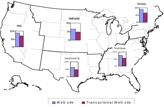
W e b s ite T r a n s a c tio n a l W e b s ite West 0% 50% 100% Sout heast 0% 50% 100% Northcentral 0% 50% 100% Northeast 0% 50% 100%

Sout hcent ral

0% 50% 100%

Figure 2: Regional Adoption for Internet Banking (2003)

of the US in 2003.3 _{The Northeast and the West have the highest adoption rates,}

while the central regions of the country have the lowest. Also banks with large size

tend to adopt IB earlier. In 2003, 96 percent of banks with assets over $300 million

reported that they had a Website, compared to only 51 percent of banks with assets

under $100 million. These observations raise an important question: what explain

these variations of diﬀusion rates across banking groups and geographic regions? Meanwhile, the diﬀusion of IB has taken place in a continuously changing

environ-ment of US banking industry. Over the past decade, several reforms of US banking

regulatory framework were introduced and expected to aﬀect the size distribution of

banks. In particular, the Riegle-Neal Interstate Banking and Branching Eﬃciency

Act was passed in September 1994. The act allows banks and bank-holding compa-3_{Data Source: Call Report (2003).}

(5)

nies to freely establish branches across state lines. This new flexibility in branching regulation has opened the door to the possibility of substantial geographical

consol-idation in the banking industry. As a result, there has been a strong trend towards

higher average bank size (Figure 1). This suggests further interesting questions: if

bank size is an important factor in the adoption of IB, then how much has banking

deregulation aﬀected IB adoption? At the same time, how much, if any, has adoption

of IB influenced the increase of average bank size?

1.2 The Hypothesis

Motivated by the aforementioned observations and questions, this paper tries to

pro-vide a general framework to study, theoretically and empirically, the endogenous

diﬀusion and impact of Internet Banking. The theory suggests that when a cost-saving technological innovation, e.g. IB, is initially introduced, large banks have an

advantage to adopt itfirst and enjoy further growth of size. Over time, due to

environ-mental changes (demand change, technological progress and industry deregulation),

the innovation gradually diﬀuses into smaller banks. As a result, the aggregate bank

size distribution increases stochastically towards a new steady state, and there are

important interactions between the IB adoption and growth of average bank size. Applying the theory to a panel study of Internet Banking diﬀusion across 50 US

states, we examine the technological, economic and institutional factors governing

the process. Using simultaneous-equation regressions, we are able to disentangle the

complex interrelationship between IB adoption and growth of average bank size, and

explain the variation of diﬀusion rates across US geographic regions.4

4_{In our empirical study, we use state-level aggregate data to estimate the IB adoption and bank} size distribution. We only include state-chartered banks in our sample to avoid the complication of

(6)

1.3 Related Literature

Several studies have looked at Internet and related technology diﬀusion in the banking

industry. Courchane, Nickerson and Sullivan (2002) develop and estimate a model

for IB adoption at the early stages when there is considerable uncertainty about

consumers’ demand. Theyfind that relative bank size and demographic information predictive of future demand positively influence IB adoption. Furst, Lang, and Nolle

(2000) estimate a logit model for the determinants of IB adoption in a sample of

national banks. They find that larger banks are more likely to adopt IB as well

as banks are younger, better performing, located in urban areas, and members of a

bank holding company. Some other studies analyze the reverse eﬀect of technology

on bank performance but obtain mixed results. Sullivan (2000) studies performance characteristics, including costs and profitability, of early adopters of IB and finds

little diﬀerence from non-adopters. Berger and Mester (2003)find that banks enjoyed

rising profits during the 1990s, and attribute this to banks’ increasing market power

gained by adopting new technologies. However, few of the existing studies have

explicitly considered the endogenous interactions between technology adoption and

bank performance measures.

This paper is afirst attempt to study the diﬀusion and impact of Internet Banking

with an equilibrium structural model. Built upon the recent work of Wang (2004)

and Olmstead and Rhode (2001), we refine the popular threshold diﬀusion model to

account for the interaction between technology adoption andfirm size. Our theory

ex-plicitly considers the heterogeneity of banks’ productivity and derives an empirically

plausible bank size distribution. Based on that, we then characterize the endogenous interstate banking. The state-chartered banks count for 75% of total commercial banks in the US, and they can be reasonally assumed to mainly serve the home states.

(7)

diﬀusion of IB and its reverse impact on the average bank size. Using the theory to construct a simultaneous-equation estimation that applies to a new dataset of IB

diﬀusion across 50 US states, the empirical results confirm our theoreticalfindings.

The approach that we develop in the paper goes far beyond the Internet Banking

by providing a general framework to study technology diﬀusion and evolution offirm

size distribution. Hence, it is also connected to a broad literature in related fields,

namely theories of industry dynamics (Hopenyahn 1992, Jovanovic and MacDonald

1994, Klepper 1996),firm size distribution (Lucas 1979, Sutton 1997, Axtell 2000) and studies of technology diﬀusion (Griliches 1957, Mansfield 1961, David 1969, Davies

1979, Manuelli and Seshadri 2003, Comin and Hohijn 2004).

1.4 Road Map

The paper is organized as follows. Section 2 presents the model, in which we study

competitive industry dynamics with endogenous technology diﬀusion. In particular,

we explore the dynamic interactions between technology adoption and change of bank

size distribution. Section 3 applies the model to a panel study on the diﬀusion of

Internet Banking across 50 US states. Using simultaneous-equation regressions, we

disentangle the complex interrelationship between IB adoption and growth of average bank size, and explain the variation of diﬀusion rates across US geographic regions.

Section 4 oﬀersfinal remarks.

2 The Model

In this section, we construct a theoretical model to study the diﬀusion and impact of

(8)

2.1 Environment

The industry is composed by a continuum of banks which produce a homogenous

product — banking service. Banks behave competitively, taking market prices as

given. We assume banks are heterogenous in the cost of production, which causes

size diﬀerences across banks. At a point of time t, the aggregate demand takes a simple form — the consumers are willing to pay Pt for the total amount Qt of the

output. Over time, the demand Pt andQt might be shifted by economic forces, such

as changes in population, income or substitute services.5

2.2 Pre-Innovation Equilibrium

Before the technology innovation arrives, the industry is at a steady state. Taking

prices as given, each individual bank maximizes profit using the existing technology:

π0 =M ax

y0

P y0−αy0β

whereπ0 is profit,P is price, y0 is output, andα >0andβ >1 are cost parameters.

Solving the maximization problem, we have

y0 = (

P αβ)

1

β−1. (1)

Given individual bank’s heterogeneity of productivity, e.g. α, there is a bank size

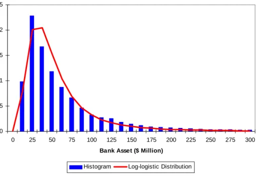
distribution G. Historically, bank size y0 fits well with a log-logistic distribution6,

5_{For simplicity, we assume consumers have inelastic demand so that}_P _and _Q_{are exogenously} determined. In fact, this is not an unreasonable assumption given our focus on state-chartered banks, a subsample of the banking population.

6_{We pick the log-logistic distribution here is not only because it serves as an easily tractable} representative of the larger group of positively skewed distributions, but also because it connects our study to the typically observed logistic diﬀusion curves. See Wang (2004) for a detailed discussion.

(9)

0 0.05 0.1 0.15 0.2 0.25 0 25 50 75 100 125 150 175 200 225 250 275 300

Bank Asset ($ Million)

Fr e q u e nc y

Histogram Log-logistic Distribution

Figure 3: Bank Size Distribution (State-Chartered Banks, 1990)

whose cdf function is given as

Gy0(x) = 1−

1

1 +b1xb2

(2)

with the mean E(y0) and Gini coeﬃcientg given as

E(y0) =b− 1/b2 1 Γ(1 + 1 b2 )Γ(1₋ 1 b2 ), g = 1 b2

where Γdenotes the gamma function Γ(μ)_≡R₀∞tμ−1_exp(

−t)dt.

Rewriting the log-logistic distribution into a more intuitive form, we have

Gy0(x) = 1−

1

1 + (ηx/E(y0))1/g

(3)

where η=Γ(1 +g)Γ(1₋g).

Figure 3 presents an example fitting the log-logistic distribution to the size

fre-quency of US state-chartered banks in 1990. As can be seen, the log-logistic

(10)

At equilibrium, aggregate demand equals supply, so that

N

Z ∞

0

y0dG(y0) =Q

where N is the total number of banks.

Notice that the assumption of log-logistic size distribution is robust to changes of

the market environment. For example, any shocks to the priceP and the mean bank

productivity7 E(α1−1β₎_{only a}_ﬀ_{ect the mean of the size distribution but nothing else;}

any shocks to the total demandQ only aﬀect the number of banks N through entry and exit, but not the size distribution.

2.3 Post-Innovation Equilibrium

2.3.1 Individual Bank Decision

At timeT, the technological innovation, Internet Banking, becomes available.

There-after, at each period an individual bank maximizes profit and decides whether to

adopt the innovation or not ( 0= do not adopt, 1= adopt):

π=M ax_{π0, π1} with π0 =M ax y0 P y0 −αy0β; π1 =M ax y1 P y1− α γy β 1 −k

whereγ is the cost saving by adopting the innovation,kis the period cost of adoption.

Solving the maximization problem, we have

y0 = ( P αβ) 1 β−1 ; π 0 = β₋1 β P y0; y1 = ( γP αβ) 1 β−1 _; _π 1 = β₋1 β P y1 −k.

7_Given_{β >}₁_,_α₁₋1β decreases withα. Hence,α

1

(11)

0 20 40 60 80 100 1999 2000 2001 2002 2003 2004 A d opt ion R a te % <$25 $25-$100 $100-$300 $300-$1000 >$1000

Figure 4: Diﬀusion of Web Sites by Bank Assets (Million)

An individual bank will adopt IB if π1 ≥π0, and there is a threshold size y0∗ for

adoption:

π1 =π0 =⇒y0∗ =

k

P(β−_β1)(γβ−11 −1)

.

The size requirement for adoption suggests that large banks have an advantage

in adopting the innovation. Using bank assets as a size approximation, we show in

Figure 4 that it is indeed what happened in the diﬀusion of Internet Banking.8

2.3.2 Aggregate Adoption

Given the log-logistic bank size distributionGdefined in Equation 3 and the threshold

y∗

0 for adoption, the aggregate adoption rate of the IB innovation is :

F = 1₋Gy0(y ∗ 0) = 1 1 + (ηy∗ 0/E(y0))1/g . (4)

(12)

Recall y0 = ( P αβ) 1 β−1; y∗ 0 = k P(β−_β1)(γβ−11 ₋₁₎ .

Then Proposition 1 follows.

Proposition 1 The adoption rateF increases with consumer demandP, mean bank

productivity E(α1−1β), cost saving γ, but decreases with adoption cost k.

Proof. Equation 4 suggests that ∂F/∂P > 0, ∂F/∂E(α1−1β) > 0, ∂F/∂γ > 0 and

∂F/∂k <0.

2.3.3 Average Bank Size

Notice E(y0) is not something directly observable. The observed mean bank size is

indeed E(y) = Z y∗ 0 0 y0dG(y0) + Z ∞ y∗ 0 y1dG(y0) =E(y0) + [γ 1 β−1 ₋_1] Z ∞ y∗ 0 y0dG(y0).

Given that y0 takes a log-logistic distributionG, we have

Z ∞

y∗ 0

y0dG(y0) =E(y0)[1−β(1 +g,1−g;G(y∗0))]

where β is the incomplete beta function defined as

β(a, b;x)_≡ Γ(a+b) Γ(a)Γ(b) Z x 0 ta−1(1₋t)b−1dt with a >0, b >0, x >0, β(a, b; 0) = 0 and β(a, b; 1) = 1.

Therefore, the observed mean bank size can be derived as follows

E(y) =E(y0){1 + [γ

1

β−1 ₋_1][1₋_β_{(1 +}_g,₁₋_g_{; 1}₋_F_)]_}_. ₍₅₎

(13)

Proposition 2 The mean bank sizeE(y) increases with consumer demandP, mean bank productivityE(α1−1β), cost saving γ, but decreases with adoption cost k.

Proof. Given Proposition 1, Equation 5 suggests that∂E(y)/∂P >0,∂E(y)/∂γ >0,

∂E(y)/∂E(α1−1β₎_>₀_and _∂E₍_y₎_{/∂k <}₀_.

2.4 Industry Dynamics and Long-run Equilibrium

Equations 4 and 5 describe the post-innovation industry equilibrium at any point of

time. Notice that we have so far omitted time subscripts of all variables. To discuss the industry dynamics, we now make them explicit. As a result, we are going to see

that the diﬀusion path closely follows a logistic curve.

In fact, over time, consumer demand Pt may change with income or substitute

services, and mean bank productivityE(α

1 1−β

t ), IB cost savingγtand IB adoption cost

ktmay change with banking deregulation and technology progress. Taking these time

changes into account, let us consider a simple law of motion with constant growth as follows Pt =P0ezpt; E(α 1 1−β t ) =E(α 1 1−β 0 )e zαt_; _γ 1 β−1 t −1 = (γ 1 β−1 0 −1)e zγt_; _k t=k0ezkt.

Then, the diﬀusion path of IB can be derived from Equation 4

Ft = 1 1 + (ηy∗ 0,t/E(y0,t))1/g = 1 1 + [ηy∗ 0,0/E(y0,0)]1/ge 1 g{zk−zα−zγ−₍_ββ₋₁₎zp}t . (6)

We may compare the diﬀusion formula derived here with the traditional logistic

model. The logistic model, based on a behavioral assumption of social contagion, assumes that the hazard rate of adoption rises with cumulative adoption

˙ Ft 1₋Ft =vFt=⇒Ft = 1 [1 + (_F1 0 −1)e −vt_] (7)

(14)

where Ft is the fraction of potential adopters who have adopted the product at time

t, and v is a constant contagion parameter.

Comparing Equation 6 with Equation 7, we realize that our diﬀusion formula is

equivalent to the logistic model under very reasonable assumptions. In particular,

the diﬀusion parameters traditionally treated as exogenous terms now have clear

economic meanings: the contagion parameterv is determined by the growth rates of

consumer demand, industry deregulation, technology progress; the initial condition

F0 is the fraction of banks thatfind it profitable to adopt the innovation at the initial

period: v= ( β (β₋1)zp+zγ+zα−zk)/g; F0 = 1 1 + [ηy∗ 0,0/E(y0,0)]1/g .

Over time, as more and more banks adopt the innovation, the mean bank size keeps rising and the aggregate size distribution of banks increases stochastically to a

new steady state. In the long run, as all banks adopt the innovation, the cumulative

distribution of bank size converges toGy1,t(x)which is still a log-logistic distribution

but with a higher mean.

Gy1,t(x) = 1− 1 1 + (Γ(1+_Eg₍)_yΓ(1−g) 1,t) x) 1/g; E(y1,t) =E(y0,t)γ 1 β−1.

Figure 5 illustrates the industry dynamic path. Before the IB innovation arrives,

the banking industry stays at a pre-innovation size distribution, drawn with a dotted

green line. After the IB innovation, in the long run, the banking industry converges to

a post-innovation long-run size distribution, drawn with a solid blue line. In between,

the banking size distribution is at a transitional path, drawn with a dashed red line. During the transition, at a point of time t, there is an critical size requirement y∗

0,t, which splits the size distribution into two parts. For banks with size y0,t ≥y0∗,t, the size distribution resembles the post-innovation long-run distribution for the range

(15)

Bank Size y Fr e que nc y G '( y ) y*0,t Pre-Innovation Distribution Post-Innovation Long-run Distribution Transitional Distribuion Maximum Size of Nonadoptor γ1/(ß-1)_y* 0,t Minimum Size of Adopter

Figure 5: Illustration of the Industry Dynamics

y1,t > γ

1

β−1y∗

0,t, while for banks with size y0,t < y0∗,t the size distribution resembles the pre-innovation one. Over time, y∗

0,t falls due to environmental changes (demand change, technology progress and banking deregulation). As a result, the IB innovation

diﬀuses into smaller banks and the bank size distribution gradually converges to the post-innovation long-run distribution.

3 Empirical Study

In this section, we apply the theoretical model to a panel data of US banking industry

and study the diﬀusion and impact of Internet Banking.

The data we use covers Internet Banking adoption (Informational Websites and Transactional Websites) among state-chartered banks across 50 US states for years

(16)

2003 and 2004, which includes about 5600 out of the total 7500 commercial banks in the US. The reason that we choose state-chartered banks is because it is more

reasonable to define the state that they receive the charter as the market they serve.

The reason that we choose the years 2003 and 2004 is because 2003 is the first year

when depository institutions were required to report their transactional Websites.

3.1 Simultaneous Equations

The diﬀusion and impact of IB can be characterized by a simultaneous equation

system, which includes an adoption equation and a size equation as follows.

Recall Equation 1 F = 1₋G(y0∗) = 1 1 + (ηy∗ 0/E(y0))1/g .

It can be rewritten into a log-linear form:

gln(1 F −1) = lnη+ ln β β₋1 + lnk−lnP −ln(γ 1 β−1 −1)−lnE(y 0). (8) Recall Equation 2 E(y) =E(y0){1 + [γ 1 β−1 ₋_1][1₋_β_{(1 +}_g,₁₋_g_{; 1}₋_F_)]_}_.

An empirical approximation of Equation 2 can be written as

lnE(y) = lnE(y0)−b1[gln(

1

F −1)] +b2ln(γ

1

β−1 −1). (9)

Therefore, Equation 8 and 9 imply

gln(1

F −1) =a0−a1lnE(y) +a1[(b2−1) ln(γ

1

β−1 −1)−lnP + lnk] (10)

(17)

Also, Equation 1 suggests y0 = ( P αβ) 1 β−1 =⇒lnE(y 0) = 1 β₋1lnP − 1 β₋1lnβ+ lnE(α 1 1−β).

Hence we can rewrite Equation 9 as

lnE(y) =b0−b1[gln( 1 F −1)] +b2ln(γ 1 β−1 −1) + 1 β₋1lnP + lnE(α 1 1−β) (11) where b0 = ₁₋1_βlnβ.

The two Equations 10 and 11 are determined simultaneously and have to be

estimated with simultaneous-equation regressions. Since the variablekis in Equation 10 but not Equation 11, and E(α1−1β) is in Equation 11 but not Equation 10, they

can be used to define exclusion restrictions and identify structural parameters.

3.2 Empirical Specifications

In the empirical study, we estimate the following simultaneous equations9 _{based on}

Equations 10 and 11 using state-level panel data 2003-2004, where each state is

indexed byj and each year is indexed by t:

gj,tln( 1₋Fj,t Fj,t ) =a0+a1ln(E(y)j,t)+ X i ailn(Xi,j,t)+ X l alln(Il,j,t)+εj,t (Adoption) ln(E(y)j,t) =b0+b1[gj,tln( 1₋Fj,t Fj,t )] +X i biln(Xi,j,t) + X l blln(Sl,j,t) +μj,t (Size)

• F is state-level adoption of IB (All Websites and Transactional Websites sepa-rately); g is the Gini coeﬃcient of state-chartered bank size distribution; 9_{Olmstead and Rhode (2001) had a similar regression setup in their study of di}_ﬀ_{usion of tractor,} but did not rationalize it with an explicit theoretical model.

(18)

• E(y) is a measure of state-level average bank size;

• X are variables shared in both equations, e.g. variables aﬀectingP andγ;

• I are variables only in theAdoption equation, e.g. variables aﬀecting k only;

• S are variables only in the Size equation, e.g. variables aﬀectingE(α1−1β)only.

The dependent variables in the two equations are as follows (Detailed explanations

and sources of empirical variables are summarized in Table 1 in the Appendix ).

(1) Log odds ratio for IB adoption adjusted by the Gini coeﬃcient, constructed

using the following variables: TRANSAVE — Adoption rate for Transactional Web-sites; WEBAVE — Adoption rate for All Websites (informational or transactional) ;

GINIASST— Gini coeﬃcient for bank assets;

(2) Average Bank Size, constructed by ASSTAVE — Bank assets10_.

As we have seen in the theory, there are four groups of exogenous variables:

consumer demand P, mean bank productivity E(α1−1β₎_{, IB cost saving} _γ _{and IB}

adoption cost k. We have to find relevant empirical variables to proxy them. The following is a preliminary grouping.

(1) Consumer Demand P: METROAVE — Ratio of banks in metropolitan areas

to all banks in state; LNSPAVE — Specialization of lending to consumers (consumer

loans plus 1-4 family mortgages / total loans); PCY — Income per capita; POPDEN

— Population density;

10_{Using Bank deposits as an alternative measure of bank size, we get very similar regression} results. See Tables 3(dep)-8(dep) in the Appendix.

(19)

(2) Mean Bank Productivity E(α1−1β₎_: _{AGEAVE — Average age of banks;}

IN-TRAREG — Indicator variable for whether the state had intrastate branching re-strictions after 1995; BHCAVE — Ratio of banks in bank holding companies to total

banks; DEPINTST — Ratio of deposits in out-of-state banks to total deposits; ASST90

— Bank assets in 1990;

(3) IB Cost Saving γ: INETADOPT — Household access rate for the Internet;

(4) IB Adoption Costk: IMITATE — Years since thefirst bank in the state adopted

a transactional Website; WAGERATIO — Wage ratio of computer analyst to teller; (5) Region dummies and Years.

Notice that the above is a preliminary grouping of variables. Some of the vari-ables may belong to more than one group. Take INETADOPT for example: if more

households have access to the Internet, local banks may get more cost savings γ

from adopting IB. However, the Internet access also allows the households to reach

non-local banking services, e.g. out-of-state banks, then may also lower the demand

P for local banking service. Another example is AGEAVE: more established banks typically achieve higher productivityα1−1β, so may have higher incentive to adopt IB.

However, they may also face higher IB adoption cost k compared to younger banks

since they have to adapt the IB to their legacy system. Therefore, we have to be

cautious to design and interpret our empirical study.

In particular, making the exclusion restrictions that define I and S becomes a

matter of economic judgement. We include two variables in I: the number of years

since thefirst bank in the state adopted a transactional Website (IMITATE) and the ratio of computer analyst wage to teller wage (WAGERATIO). They are expected

to aﬀect the bank size only through the IB adoption. In S, we use four variables:

(20)

1995 (INTRAREG); the ratio of banks in bank holding companies to total banks (BHCAVE); the ratio of deposits in out-of-state banks to total deposits (DEPINTST);

and bank assets in 1990 (ASST90). They are expected to aﬀect the adoption of IB

only through their eﬀects on average bank size.

3.3 Data and Estimation Details

We run simultaneous-equation regressions on a sample panel dataset. The sample

consists of state-chartered, full service retail banks across 50 states of the US. Table

2 in the Appendix shows summary statistics for all empirical variables.

As the theory suggests, we use Gini-adjusted log-odds ratio as the dependent

variable. However, by the year 2004 four states had achieved full adoption of

trans-actional Websites, so that the log-odds ratio can not be calculated. Hence, there are 92 observations in the transactional IB estimation instead of 100. For the same

reason, there are 82 observations in the all IB (informational or transactional)

esti-mation. Also, for most empirical variables used in the estimation, we take the log

transformation and prefix the variables with “ln” in the notation.

To get robust estimates, we conduct regressions using various definitions of

depen-dent variables as well as diﬀerent model setups. For the dependent variables, we use Transactional Websites and All Websites (informational or transactional) as

alterna-tive measures of IB adoption, and use Bank Assets and Bank Deposits as alternaalterna-tive

measures of bank size. For the regressions, we estimate three diﬀerent setups

includ-ing a simultaneous-equation model on a pooled cross-section and time-series data,

a random-eﬀect simultaneous-equation panel model, and simple OLS regressions on

two structural equations. Tables 3-5 in the Appendix report regression results with three model setups using Transactional Websites and Bank Assets as dependent

(21)

vari-ables; Tables 6-8 use All Websites (informational or transactional) and Bank Assets as dependent variables; Tables 3(dep)-8(dep) repeat the regressions in Tables 3-8 but

use Bank Deposits instead of Bank Assets as the measure of bank size.

3.4 Estimation Results

In the following discussion, we mainly refer to results in Table 3-5, which use Trans-actional Websites and Bank Assets as dependent variables. Results in other tables

are similar, and are used as supporting evidence whenever necessary.

Looking first at Table 5, which reports simple OLS regression results on two

structural equations without taking care of the potential simultaneity problem. The

coeﬃcients of IB adoption (lnTRANODDS*GINIAVE) and bank size (lnASSTAVE)

are both found to be statistically significant. It confirms our hypothesis that IB adop-tion and bank size are simultaneously determined, and suggests that OLS estimates

may be inconsistent. To obtain consistent estimates, we use simultaneous-equation

techniques and report results in Tables 3-4. The main results are similar in the two

tables and we would therefore focus discussion on Table 3.

Table 3 presents results of estimating the model using instrumental variables where

the IB adoption rate is measured with Transactional Websites. For completeness we present estimates of reduced form equations but will focus on discussing estimated

structural equations. Overall, the structural model has a goodfit with a R-square of

72 percent for the adoption equation and 78 percent for the size equation. Most of

the signs of estimated coeﬃcients, and all of those that are statistically significant,

are consistent with our theoretical predictions.

We turnfirst to the structural equation for IB adoption (Table 3, column 3). The coeﬃcient on the fitted value of lnASSTAVE is negative and statistically diﬀerent

(22)

from zero. An increase in a state’s average bank assets is associated with a fall in the odds ratio for transactional Website adoption. Consistent with our theoretical

model, this implies a rise in the adoption rate.

In the structural equation for average bank assets (Table 3, column 4), the coeﬃ

-cient on the fitted value of lnTRANSAVE*GINIASST is also negative, as expected,

though not statistically diﬀerent from zero. However, we should have confidence with

the negative eﬀect, since the simple OLS regressions in Table 5 have shown that zero

eﬀect is not consistent with the data and we consistently get negative coeﬃcient esti-mates using all alternative regressions. Moreover, when adoption rates are measured

using All Websites (informational or transactional), the coeﬃcient turns statistically

significant (Table 6, column 4).

There is a negative coeﬃcient on lnIMITATE (Table 3, column 3). The result

implies that the longer the state has had a bank with a Transactional Website, the

higher the state’s Internet Banking adoption rate. The leadership of the early adopter may have helped prepare other banks and customers to use Internet Banking through

lowering the adoption cost, financially or perceptionally.

Estimates show strong persistence in the asset size distribution across states. The

estimated positive coeﬃcient on lnASST90 (Table 3, column 4), which is statistically

diﬀerent from zero, implies that the average bank assets of a state in 1990 is a good

predictor of average assets in 2003 and 2004. Estimates suggest that interstate com-petition (lnDEPINTST) has a negative influence on the asset size of a state’s banks.

Although the eﬀect is not statistically significant, it turns significant when adoption

rates are measured using All Websites (informational or transactional) (Table 6,

col-umn 4). Neither intrastate branching restrictions (INTRAREG) after 1995 nor BHC

(23)

structural equation, but BHC membership is shown to have significantly positive eﬀects on IB adoption and bank assets in the reduced form regressions.

Explanatory variable that describe bank characteristics have a mixed impact on

Website adoption and average asset size. Our measure of the location of banks in

metropolitan areas (lnMETRO) seems to positively aﬀect both bank size and IB

adop-tion, though not statistically significant in either structural equation. The significant

negative coeﬃcient on lnLNSPAVE in the asset size equation (Table 3, column 4)

im-plies that greater specialization of a state’s banks in consumer lending is associated with a smaller average bank assets. Perhaps banks achieve greater average size with

lending focused on other areas, such as commercial loans. The significant negative

coeﬃcient on lnLNSPAVE in the Website adoption equation suggests that greater

spe-cialization of a state’s banks in consumer lending is associated with a higher adoption

rate. This is consistent withfindings that early bank Websites oﬀered services aimed

at retail customers and later added features useful to businesses (Sullivan (2004)). The average age of a state’s banks is significantly related to both Website

adop-tion and asset size. The positive coeﬃcient on lnAGEAVE in the Website adoption

equation implies that as the average age of a state’s banks rises then the adoption rate

falls. This results is consistent with previous findings that denovo banks were more

likely to adopt Internet Banking than other banks (Furst, Lang, and Nolle (2000);

Sullivan (2000)). New banks mayfind it cheaper to install Internet Banking technol-ogy in a package with other computer facilities compared to older banks who must

add Internet Banking to legacy computer system. Many new banks may also

pur-sue consumers with demographics that favor Internet Banking and therefore adopt

appropriate technology.

(24)

of a state have expected signs and are statistically significant for both the Website adoption and the asset size equation. A state’s per capita income (lnPCY) is

pos-itively related to the average asset size of banks but is not significantly related to

Website adoption. Population density (lnPOPDEN) is also positively related to asset

size but negatively related to Website adoption. The latter result implies that

adop-tion of Internet Banking is higher where populaadop-tion is less dense, which is consistent

with a higher demand for Internet Banking in locations with higher cost of travel to

bank branches.

Finally, access of households to the Internet (lnINETADPT) is statistically

sig-nificant in explaining both Website adoption and asset size in sample states. Greater

household access to the Internet is associated with a higher Website adoption rate, as

expected. On these estimates, greater household access to the Internet is negatively

related to a state’s average bank assets. A possible explanation is that once on the

Internet a household has an opportunity to form a relationship with bank outside of their home state, which may have a negative impact on the size of banks in their

home state.

3.5 Empirical Findings on IB Di

ﬀ

usion

The estimation results have confirmed our theoretical findings. First, there are

im-portant interrelationship between IB adoption and average bank size. Quantitatively,

as shown in Table 3, a 10 percent increase in average bank size would decrease the

Gini-adjusted adoption odds ratio by about 1.4 percent, and a 10 percent decrease of

adoption odds ratio would increase the average bank size by about 3.7 percent. The

eﬀects become even stronger when IB adoption rates are measured using All Websites (informational or transactional).

(25)

Since the IB adoption and bank size are endogenous variables, they are determined by underlying technological, economic and institutional factors. In the theory, we have

grouped those factors into four basic categories that aﬀect, respectively, consumer

demandP, mean bank productivity E(α1−1β), IB cost savingγ and IB adoption cost

k. The empiricalfindings then reveal their quantitative eﬀects.

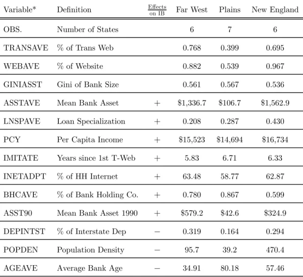
Table 9a: Mean Values of Selected Variables Across Regions (Far West, Plains and New England 2003)

Variable* Definition E_{on IB}ﬀects Far West Plains New England

OBS. Number of States 6 7 6

TRANSAVE % of Trans Web 0.768 0.399 0.695

WEBAVE % of Website 0.882 0.539 0.967

GINIASST Gini of Bank Size 0.561 0.567 0.536

ASSTAVE Mean Bank Asset + $1,336.7 $106.7 $1,562.9

LNSPAVE Loan Specialization + 0.208 0.287 0.430

PCY Per Capita Income + $15,523 $14,694 $16,734

IMITATE Years since 1st T-Web + 5.83 6.71 6.33

INETADPT % of HH Internet + 63.48 58.77 62.87

BHCAVE % of Bank Holding Co. + 0.780 0.867 0.599

ASST90 Mean Bank Asset 1990 + $579.2 $42.6 $324.9

DEPINTST % of Interstate Dep ₋ 0.319 0.164 0.294

POPDEN Population Density ₋ 95.7 39.2 470.4

AGEAVE Average Bank Age ₋ 34.91 80.18 57.46

*See Table 1 for details of variable definitions and sources.

(26)

rates across US geographic regions? To be specific, why do the Northeast and the West have the highest IB adoption rates, while the central regions of the country

have the lowest? To answer this question, we present regional average of variables

that are found significantly aﬀecting IB adoption in our regressions in Table 9a, in

which we use Far West, Plains and New England to represent the West, Central and

Northeast regions respectively.

The data in Table 9a shows that in 2003 the Plains region has a similar number

of states and a similar Gini coeﬃcient of bank size distribution compared to the other two regions, but the average IB adoption rate in the Plains region was only

about half of that of the other two regions. Compared with the Far West and New

England, the Plains region has smaller mean bank size, lower per capita income,

lower household access to Internet and older bank vintages. All these factors appear

to have contributed to slow diﬀusion of Internet Banking.

However, at the same time, the data reject several alternative explanations of slow IB diﬀusion in the Central regions. In particular, it is not caused by the imitation of

early adopters, percentage of BHC membership, competition from out-of-state banks

or population density. In fact, all those factors work in favor of adopting Internet

Banking in the Central region.

In a similar way, we can also compare variations of IB diﬀusion rates between

any other regions. Average value of variables for all eight US regions are reported in Table 9 in the Appendix.

Interestingly, after we control for other factors, most regional dummies are not

statistically significant explaining bank size or IB adoption. One exception is the Far

West. Some regional fixed eﬀect may have played significant roles in promoting IB

(27)

4 Final Remarks

This paper studies the endogenous diﬀusion and impact of Internet Banking. When a

cost-saving innovation, such as Internet Banking, is initially introduced, large banks

have an advantage to adopt it first and enjoy further growth of size. Over time,

due to environmental changes (demand change, technology progress and banking

deregulation), the innovation diﬀuses into smaller banks. As a result, the aggregate bank size distribution increases stochastically towards a new steady state, and there

exists important interactions between the IB adoption and the average bank size.

Applying the theory to a panel study of the diﬀusion of IB across 50 US states, we

examine the technological, economic and institutional factors governing the process.

Using simultaneous-equation regressions, we are able to disentangle quantitatively

the complex relationship between IB adoption and growth of average bank size, and explain the variation of IB diﬀusion rates across geographic regions. Wefind that the

factors significantly aﬀecting IB adoption include mean bank size, per capita income,

household access to Internet, average bank age, bank loan specialization, imitation of

early adopters, percentage of BHC membership, competition from out-of-state banks

and population density. In particular, it is the first four factors that are primarily

responsible for the slower diﬀusion of Internet Banking in the Central region than the West and Northeast regions.

The theoretical and empirical approach that we develop in the paper goes far

beyond the Internet Banking. It indeed provides a general framework to study the

joint evolution of technology adoption and firm size distribution, and can be readily

(28)

References

[1] Axtell, Robert L. (2000). “Zipf Distribution of U.S. Firm Sizes,” Science, 293:

1818-1820.

[2] Berger, Allen and Robert DeYoung (2002). “Technological Progress and the

Geo-graphic Expansion of the Banking Industry,”Finance and Economics Discussion

Series, 2002-31, Federal Reserve Board.

[3] Berger, Allen and Loretta Mester (2003). “Explaining the Dramatic Changes of

Performance of U.S. Banks: Technological Change, Deregulation and Dynamic

Changes in Competition,” Journal of Financial Intermediation, Vol. 12(1), pp

57-95.

[4] Comin, D. and Hohijn B., (2004). “Cross-Country Technological Adoption: Mak-ing the Theories Face the Facts,”Journal of Monetary Economics, January 2004,

pp. 39-83.

[5] Courchane, Marsha, David Nickerson and Richard J. Sullivan, (2002).

“Invest-ment in Internet Banking as a Real Option: Theory and Tests.” The Journal of

Multinational Financial Management, 12 (4-5), Oct.-Dec., pp. 347-63. [6] David, Paul, (1969). “A Contribution to the Theory of Diﬀusion,” mimeo.

[7] Davies, Stephen. (1979).The Diﬀusion of Process Innovations,Cambridge

Uni-versity Press.

[8] Furst, Karen, William Lang, and Daniel Nolle (2001). “Internet Banking in the

U.S.: Landscape, Prospects, and Industry Implications,” Journal of Financial

(29)

[9] Fisk, Peter R., (1961). “The Graduation of Income Distributions,”Econometrica, 29, 2, 171-185.

[10] Griliches, Zvi, (1957). “Hybrid Corn: An Exploration in the Economics of

Tech-nological Change,”Econometrica, 25, (Oct.), 501-522.

[11] Harker, Patrick and Baba Prasad (1997). “Mxamining the Contribution of

Infor-mation Technology Toward Productivity and Profitability in U.S. Retail

Bank-ing,”Working paper 97-09, Wharton Financial Institutions Center, The Wharton

School.

[12] Hopenhayn, H. A. (1992). “Entry, Exit, and Firm Dynamics in Long Run Equi-librium,”Econometrica, 60(2): 1127-1150.

[13] Jovanovic, Boyan and G. M. MacDonald, (1994). “The Life Cycle of a

Compet-itive Industry,”Journal of Political Economy, 102 (Apr.), 322-347.

[14] Klepper, Steven, (1996). “Entry, Exit, Growth, and Innovation over the Product

Life Cycle,” American Economic Review, 86 (June), 562-583.

[15] Lucas, Robert E., (1978). “On the Size Distribution of Business Firms,” The

Bell Journal of Economics, 9, 2, 508-523.

[16] Mansfield, Edwin, (1961). “Technical Change and the Rate of Imitation,”

Econo-metrica, 29 (Oct.), 741-766.

[17] Mansfield, Edwin, (1962). “Entry, Gibrat’s Law, Innovation, and the Growth of

Firms,”American Economic Review, 52 (Dec.), 1023-51.

[18] Manuelli, Rodolfo and Ananth Seshadri, (2003). “Frictionless Technology Diﬀ

(30)

[19] Olmstead, Alan and Paul Rhode, (2001). “Reshaping the Landscape: The Im-pact and Diﬀusion of the Tractor in American Agriculture, 1910-1960,” The

Journal of Economic History, Vol. 61, No. 3. p663-698.

[20] Rogers, Everett (1995). Diﬀusion of Innovations, 4th Edition. Free Press, New

York.

[21] Stiroh, Kevin (2002). “Information Technology and the U. S. Productivity Re-vival: What do the Industry Data Say?” American Economic Review, Vol. 92(5),

pp 1559-1576.

[22] Sullivan, Richard, (2004). “Payment Services and the Evolution of Internet

Bank-ing,”Payments System Reserch Briefing, (Aug.), Federal Reserve Bank of Kansas

City.

[23] Sullivan, Richard, (2000). “How Has the Adoption of Internet Banking Aﬀected

Performance and Risk in Banks? A Look at Internet Banking in the Tenth

Federal Reserve District,”Financial Industry Perspective, Federal Reserve Bank

of Kansas City.

[24] Sutton, John, (1997). “Gibrat’s Legacy,”Journal of Economic Literature, 35(1), pp. 40-59.

[25] Wang, Zhu. (2005) “Technology Innovation and Market Turbulence: A Dotcom

Example,”Working Paper, Payments System Research Department, Federal

Re-serve Bank of Kansas City.

[26] Wang, Zhu. (2004) “Learning, Diﬀusion and Industry Life Cycle,”Ph.D. Disser-tation, Department of Economics, University of Chicago.

(31)

Table 1

Empirical Variable Definitions and Sources

Variable name Definition Source

TRANSAVE Adoption rate for transactional Web sites Call Report

TRANODDS Odds ratio for adoption of transactional Web sites Call Report

WEBAVE Adoption rate information and transactional Web sites Call Report

WEBODDS Odds ratio for adoption of information and transactional Web sites Call Report

GINIASST Gini coefficient for bank assets Call Report

ASSTAVE Bank assets Call Report

METROAVE Ratio of banks in metropolitan areas to all banks in state Call Report LNSPAVE Specialization of lending to consumers (consumer loans plus 1-4

family mortgages / total loans)

Call Report

PCY Income per capita (in 1980-82 dollar) Statistical Abstract of the United States

POPDEN Population density Statistical Abstract

of the United States IMITATE Years since the first bank in the state adopted a transactional Web

site

Online Banking Report

AGEAVE Age of banks Call Report

INETADOPT Household access rate for Internet Statistical Abstract

of the United States

WAGERATIO Ratio of computer analyst wage to teller wage Bureau of Labor

Statistics

INTRAREG Indicator variable for whether the state had branching restrictions after 1995

FDIC

BHCAVE Ratio of banks in bank holding companies to total banks Call Report DEPINTST Ratio of deposits in out-of-state banks to total deposits FDIC Summary of

Deposits ASST90 Bank assets in 1990 Call Report

YEAR Year Call Report

SE Indicator variable for states located in the Southeast (AL, AR, FL,

GA, KY, LA, MS, NC, SC, TN, VA, WV)

Bureau of Economic Analysis

FARWEST Indicator variable for states located in the Far Western region (AK, CA, HI, NV, OR, WA)

ROCKYMTN Indicator variable for states located in the Rocky Mountain region

(CO, ID, MT, UT, WY)

SW Indicator variable for states located in the Southwest (AZ, NM,

OK, TX)

NWENGLND Indicator variable for states located in New England (CT, MA, ME, NH, RI, VT)

MIDEAST Indicator variable for states located Middle Eastern region (DC, DE, MD, NJ, NY, PA)

GRTLAKE Indicator variable for states located in the Great Lakes region (IL,

IN, MI, OH, WI)

Notes: data are for individual states. Data for banks are unweighted averages for those located in individual states. Selected banks were state-chartered, full-service, retail commercial banks.

(32)

Table 2 Summary Statistics

2003 2004

VARIABLE Obs Mean Std. Dev. Min Max Obs Mean Std. Dev. Min Max

TRANSAVE 50 0.573 0.166 0.277 1.000 50 0.671 0.169 0.353 1.000 TRANODDS 50 0.898 0.577 0.000 2.615 50 0.592 0.428 0.000 1.831 WEBAVE 50 0.757 0.162 0.443 1.000 50 0.813 0.153 0.471 1.000 WEBODDS 50 0.391 0.346 0.000 1.259 50 0.282 0.287 0.000 1.121 GINIASST 50 0.618 0.153 0.298 0.922 50 0.620 0.153 0.307 0.914 ASSTAVE* 50 $837.9 $1,648.0 $78.3 $9,485.8 50 $799.5 $1,292.7 $85.1 $6,023.8 METROAVE 50 0.759 0.190 0.264 1.000 50 0.763 0.190 0.264 1.000 LNSPAVE 50 0.365 0.120 0.130 0.609 50 0.355 0.120 0.124 0.591 PCY 50 $14,822 $1,819 $11,777 $19,816 50 $15,191 $1,881 $12,082 $20,412 POPDEN 50 187 256 1 1165 50 188 258 1 1173 IMITATE 50 6.700 1.111 4 9 50 7.700 1.111 5 10 AGEAVE 50 56.6 23.3 5.1 95.7 50 56.7 23.7 5.9 96.7 INETADPT 50 57.999 5.868 43.549 69.422 50 63.956 5.564 50.673 73.493 WAGERATIO 50 3.024 0.243 2.343 3.464 50 3.058 0.250 2.520 3.699 INTRAREG 50 0.240 0.431 0 1 50 0.240 0.431 0 1 BHCAVE 50 0.772 0.139 0.308 1.000 50 0.780 0.136 0.333 1.000 DEPINTST 50 0.278 0.187 0.002 0.741 50 0.328 0.201 0.003 0.840 ASST90* 50 $292.0 $504.4 $29.6 $2,451.2 50 $292.0 $504.5 $29.6 $2,451.2 YEAR 50 2003 0 2003 2003 50 2004 0 2004 2004 SE 50 0.240 0.431 0 1 50 0.240 0.431 0 1 FARWEST 50 0.120 0.328 0 1 50 0.120 0.328 0 1 ROCKYMTN 50 0.100 0.303 0 1 50 0.100 0.303 0 1 SW 50 0.080 0.274 0 1 50 0.080 0.274 0 1 NWENGLND 50 0.120 0.328 0 1 50 0.120 0.328 0 1 MIDEAST 50 0.100 0.303 0 1 50 0.100 0.303 0 1 GRTLAKE 50 0.100 0.303 0 1 50 0.100 0.303 0 1

Notes: Sample includes the 50 states in the U.S. See Table 1 for variable definitions and sources. *In millions.

(33)

Table 3

Simultaneous Equation Model of Adoption of Transactional Websites and Average Bank Assets Instrumental Variables Estimates

Reduced Forms Structural Equations

Dependent variable: lnTRANODDS*GINIAVE lnASSTAVE lnTRANODDS*GINIAVE lnASSTAVE

lnASSTAVE (fitted) -0.1445*

(0.0725)

lnTRANODDS*GINIAVE (fitted) -0.3662

(0.9122) lnIMITATE -0.5661** 0.1401 -0.4852** (0.2255) (0.4804) (0.2298) lnWAGERATIO -0.3157 2.2477* 0.1127 (0.3830) (1.1528) (0.4299) INTRAREG -0.0227 0.0893 0.0235 (0.0926) (0.2039) (0.2013) lnASST90 -0.1482 0.7778*** 0.6761*** (0.0954) (0.1545) (0.1920) lnBHCAVE -0.8057*** 1.1954* 0.9286 (0.2592) (0.6196) (0.9658) lnDEPINTST -0.0812** -0.1239* -0.1628 (0.0320) (0.0662) (0.1028) lnMETROAVE -0.2434 0.2373 -0.1904 0.1074 (0.2387) (0.4001) (0.1925) (0.4787) lnLNSPECAVE -0.2341 -0.4953 -0.3419* -0.7074* (0.1497) (0.4449) (0.1910) (0.4045) lnAGEAVE 0.3795*** 0.4946** 0.4183*** 0.6718** (0.1335) (0.2353) (0.1230) (0.3310) lnPCY 0.0279 2.0679** 0.3348 1.9618** (0.4447) (0.9207) (0.4843) (0.9646) lnPOPDEN 0.0734 0.2693* 0.1314* 0.3156** (0.0677) (0.1579) (0.0664) (0.1316) lnINETADPT -0.9300* -3.7095*** -1.6319*** -3.3892** (0.5556) (1.2342) (0.5284) (1.6507) SE -0.1455 0.5984** -0.1193 0.6322* (0.1471) (0.2734) (0.1735) (0.3703) FARWEST -0.5631*** 1.0452*** -0.4828** 0.8041 (0.1582) (0.2948) (0.1886) (0.5095) ROCKYMTN -0.0449 1.1088*** 0.0876 1.0561*** (0.1442) (0.3275) (0.1543) (0.3489) SW 0.1123 -0.0088 0.0221 0.1328 (0.1378) (0.2215) (0.1362) (0.2345) NWENGLND -0.0344 0.5222 0.1492 0.5050 (0.2037) (0.3833) (0.1757) (0.4010) MIDEAST -0.3224 -0.4515 -0.3767* -0.2785 (0.2612) (0.4362) (0.2209) (0.5260) GRTLAKE -0.0935 0.1138 -0.1394 0.2077 (0.1345) (0.2655) (0.1425) (0.2891) YEAR -0.0897 0.3355** -0.0588 0.2523 (0.0792) (0.1572) (0.0830) (0.1989) CONSTANT 183.89 -679.88** 121.09 -510.85 (159.48) (315.25) (167.23) (401.16) Observations 92 92 92 92 R-squared 0.77 0.79 0.72 0.78

Robust standard errors in parentheses. See Table 1 for variable definitions and sources. * significant at 10%; ** significant at 5%; *** significant at 1%.

(34)

Table 4

Simultaneous Equation Model of Adoption of Transactional Websites and Average Bank Assets

Random Effects Model using Generalized Least Squares

Structural Equations

Dependent variable: lnTRANODDS*GINIAVE lnASSTAVE

lnASSTAVE (fitted) -0.1449**

(0.0626)

(0.7756) lnIMITATE -0.4760* (0.2747) lnWAGERATIO 0.1526 (0.4484) INTRAREG 0.1698 (0.2970) lnASST90 0.8148*** (0.2272) lnBHCAVE 0.3925 (0.8277) lnDEPINTST -0.0586 (0.0852) lnMETROAVE -0.1896 0.5202 (0.2526) (0.7227) lnLNSPECAVE -0.2998 -0.0450 (0.2225) (0.5594) lnAGEAVE 0.4013*** 0.6698** (0.1329) (0.2671) lnPCY 0.3329 1.1476 (0.5310) (1.3452) lnPOPDEN 0.1256* 0.1512 (0.0729) (0.2174) lnINETADPT -1.6154*** -2.1535* (0.6180) (1.2558) SE -0.1347 0.3457 (0.2023) (0.5560) FARWEST -0.4750** 0.8040 (0.1975) (0.6440) ROCKYMTN 0.0740 0.6490 (0.1720) (0.5566) SW 0.0096 -0.1752 (0.1841) (0.5066) NWENGLND 0.1336 -0.0412 (0.2026) (0.6425) MIDEAST -0.3885* -0.5833 (0.2153) (0.7946) GRTLAKE -0.1511 0.0417 (0.1866) (0.5492) YEAR -0.0599 0.1995 (0.0772) (0.1771) Constant 123.44 -402.09 (153.95) (353.27) Observations 92 92 R-squared 0.72 0.76

Standard errors in parentheses. See Table 1 for variable definitions and sources.

(35)

Table 5

Single Equation Models of Adoption of Transactional Websites and Average Bank Assets

Ordinary Least Squares Estimates

Dependent variable: lnTRANODDS*GINIAVE lnASSTAVE

lnASSTAVE -0.1339** (0.0555) lnTRANODDS*GINIAVE -0.5603** (0.2537) lnIMITATE -0.4850** (0.2310) lnWAGERATIO 0.0962 (0.4221) INTRAREG 0.0199 (0.2030) lnASST90 0.6491*** (0.1810) lnBHCAVE 0.7741 (0.6094) lnDEPINTST -0.1778** (0.0823) lnMETROAVE -0.1987 0.0434 (0.1899) (0.4182) lnLNSPECAVE -0.3347* -0.7114* (0.1864) (0.4038) lnAGEAVE 0.4143*** 0.7154*** (0.1208) (0.2340) lnPCY 0.3255 1.9220* (0.4890) (0.9962) lnPOPDEN 0.1292* 0.3213** (0.0659) (0.1358) lnINETADPT -1.6011*** -3.5946*** (0.5312) (1.2315) SE -0.1308 0.5793* (0.1624) (0.3093) FARWEST -0.4957*** 0.7114** (0.1745) (0.3040) ROCKYMTN 0.0781 1.0382*** (0.1476) (0.3150) SW 0.0209 0.1319 (0.1360) (0.2382) NWENGLND 0.1350 0.4992 (0.1602) (0.3947) MIDEAST -0.3931* -0.3448 (0.2151) (0.4351) GRTLAKE -0.1494 0.1722 (0.1348) (0.2683) YEAR -0.0620 0.2237 (0.0843) (0.1576) Constant 127.46 -452.36 (169.87) (316.69) Observations 92 92 R-squared 0.72 0.78 Robust standard errors in parentheses. See Table 1 for variable definitions and sources.

(36)

Table 6

Simultaneous Equation Model of Adoption of Informational or Transactional Websites and Average Bank Assets

Instrumental Variables Estimates

Dependent variable: lnWEBODDS*GINIAVE lnASSTAVE lnWEBODDS*GINIAVE lnASSTAVE

lnASSTAVE (fitted) -0.2498**

(0.0969)

lnWEBODDS*GINIAVE (fitted) -1.3587**

(0.6613) lnIMITATE -0.7578** 0.6417 -0.4311 (0.3371) (0.5322) (0.2710) lnWAGERATIO -0.8403* 2.3330* -0.1374 (0.4718) (1.2836) (0.4608) INTRAREG -0.0307 0.1419 0.0648 (0.1135) (0.1811) (0.1486) lnASST90 -0.3958*** 0.8252*** 0.2794 (0.0925) (0.1637) (0.2745) lnBHCAVE -0.4848 -0.1173 -0.6859 (0.4422) (0.5407) (0.6379) lnDEPINTST -0.1131*** -0.0923 -0.2444** (0.0381) (0.0619) (0.0990) lnMETROAVE 0.2456 -0.2650 0.0059 -0.0596 (0.2686) (0.3894) (0.2056) (0.3855) lnLNSPECAVE -0.4597* 0.2990 -0.2441 -0.2741 (0.2644) (0.4228) (0.2364) (0.3705) lnAGEAVE 0.5823** -0.2981 0.3480 0.3646 (0.2603) (0.3564) (0.2096) (0.3946) lnPCY 0.8275 0.6025 0.7321 1.3679 (0.5958) (0.9183) (0.5475) (0.8367) lnPOPDEN 0.0948 0.0210 0.0624 0.1352 (0.0969) (0.1357) (0.0905) (0.1061) lnINETADPT -1.7127** -2.7048** -2.6341*** -4.5636*** (0.6644) (1.2193) (0.7277) (1.6887) SE -0.1724 0.1780 -0.4129* -0.1016 (0.1732) (0.2960) (0.2147) (0.3730) FARWEST -0.6106** 0.6868** -0.6144** -0.1743 (0.2389) (0.2842) (0.2414) (0.4602) ROCKYMTN 0.0267 0.4102 -0.0483 0.3528 (0.2583) (0.3099) (0.2522) (0.2749) SW 0.1457 -0.2703 -0.1278 -0.0619 (0.1550) (0.2034) (0.1611) (0.2330) NWENGLND -1.3722*** 1.6579*** -1.3430*** -0.2179 (0.2622) (0.4181) (0.4071) (0.9481) MIDEAST -0.4221 -0.3978 -0.7890*** -0.8067 (0.3038) (0.3365) (0.2579) (0.5028) GRTLAKE -0.2893** 0.3054 -0.3748** -0.0530 (0.1193) (0.2217) (0.1703) (0.3466) YEAR 0.0431 0.2493 0.0934 0.2305* (0.0949) (0.1517) (0.0879) (0.1278) CONSTANT -84.30 -494.01 -181.55 -450.68* (190.86) (304.31) (176.14) (256.47) Observations 82 82 82 82 R-squared 0.86 0.85 0.86 0.87 Robust standard errors in parentheses. See Table 1 for variable definitions and sources.

(37)

Table 7

Simultaneous Equation Model of Adoption of Informational or Transactional Websites and Average Bank Assets

Dependent variable: lnWEBODDS*GINIAVE lnASSTAVE

lnASSTAVE (fitted) -0.2483***

(0.0716)

lnWEBODDS*GINIAVE (fitted) -0.6501

(0.9309) lnIMITATE -0.3990 (0.2969) lnWAGERATIO -0.1305 (0.4930) INTRAREG 0.1239 (0.2526) lnASST90 0.6611** (0.3060) lnBHCAVE 0.0002 (0.7685) lnDEPINTST -0.0649 (0.0627) lnMETROAVE 0.0039 0.1862 (0.2558) (0.7270) lnLNSPECAVE -0.2328 0.1087 (0.2425) (0.4685) lnAGEAVE 0.3414* 0.1941 (0.2007) (0.4911) lnPCY 0.6712 1.2014 (0.6034) (1.3582) lnPOPDEN 0.0549 0.0012 (0.0877) (0.2290) lnINETADPT -2.5128*** -2.8287 (0.6658) (1.7299) SE -0.4044* 0.0513 (0.2117) (0.6106) FARWEST -0.6143*** 0.1786 (0.2129) (0.7175) ROCKYMTN -0.0619 0.1664 (0.2009) (0.5708) SW -0.1194 -0.1845 (0.1866) (0.4561) NWENGLND -1.3243*** 0.4142 (0.3925) (1.5875) MIDEAST -0.7751*** -0.6632 (0.2428) (0.8475) GRTLAKE -0.3673* 0.0967 (0.1955) (0.6301) YEAR 0.0690 0.1991 (0.0851) (0.1518) Constant -132.74 -395.12 (170.62) (303.41) Observations 82 82 R-squared 0.86 0.87 Standard errors in parentheses. See Table 1 for variable definitions and sources.

(38)

Table 8

Single Equation Models of Adoption of Informational or Transactional Websites and Average Bank Assets

Dependent variable: lnWEBODDS*GINIAVE lnASSTAVE

lnASSTAVE -0.2863*** (0.0701) lnWEBODDS*GINIAVE -0.9019*** (0.1504) lnIMITATE -0.4128 (0.2619) lnWAGERATIO -0.0632 (0.4412) INTRAREG 0.0728 (0.1472) lnASST90 0.4478** (0.1751) lnBHCAVE -0.4966 (0.5276) lnDEPINTST -0.1977*** (0.0672) lnMETROAVE 0.0218 -0.1141 (0.2037) (0.3464) lnLNSPECAVE -0.2521 -0.2166 (0.2359) (0.3522) lnAGEAVE 0.3443 0.2234 (0.2098) (0.3037) lnPCY 0.7323 1.2519 (0.5439) (0.8087) lnPOPDEN 0.0654 0.1331 (0.0885) (0.1034) lnINETADPT -2.6904*** -3.8292*** (0.6870) (1.2059) SE -0.3751* 0.0515 (0.1947) (0.3160) FARWEST -0.5757*** 0.0688 (0.2118) (0.2578) ROCKYMTN -0.0275 0.4029 (0.2366) (0.2532) SW -0.1253 -0.0682 (0.1588) (0.2135) NWENGLND -1.2151*** 0.3363 (0.3177) (0.4436) MIDEAST -0.7254*** -0.6116* (0.2244) (0.3383) GRTLAKE -0.3357** 0.1205 (0.1471) (0.2394) YEAR 0.0981 0.2565** (0.0849) (0.1265) Constant -190.46 -505.75* (170.26) (253.72) Observations 82 82 R-squared 0.86 0.88 Robust standard errors in parentheses. See Table 1 for variable definitions and sources.

(39)

Table 9

Mean Values of Selected Variables by Region 2003

VARIABLE New England Mideast Southeast Great Lakes Plains

Rocky

Mountain Southwest Far West United States

TRANSAVE 0.695 0.686 0.522 0.533 0.399 0.559 0.485 0.768 0.573 TRANODDS 0.528 0.487 0.992 0.931 1.646 0.850 1.235 0.337 0.898 WEBAVE 0.967 0.894 0.718 0.722 0.539 0.749 0.640 0.882 0.757 WEBODDS 0.038 0.121 0.409 0.404 0.921 0.346 0.666 0.155 0.391 GINIASST 0.536 0.691 0.677 0.765 0.567 0.529 0.572 0.561 0.618 ASSTAVE* $1,562.9 $2,536.5 $568.6 $558.6 $106.7 $174.6 $144.5 $1,336.7 $837.9 METROAVE 0.857 0.958 0.690 0.782 0.510 0.688 0.766 0.958 0.759 LNSPAVE 0.430 0.422 0.446 0.451 0.287 0.290 0.307 0.208 0.365 PCY $16,734 $17,066 $13,422 $14,920 $14,694 $14,072 $13,332 $15,523 $14,822 POPDEN 470.4 565.8 132.4 191.6 39.2 20.1 50.0 95.7 187 IMITATE 6.33 7.20 7.00 7.80 6.71 6.00 6.50 5.83 6.700 AGEAVE 57.46 53.75 55.13 76.43 80.18 44.05 44.98 34.91 56.6 INETADPT 62.87 60.84 52.11 56.41 58.77 61.29 53.09 63.48 57.999 WAGERATIO 2.81 3.21 3.01 3.17 3.10 2.97 2.98 2.97 3.024 INTRAREG 0.0 0.2 0.3 0.0 0.6 0.6 0.3 0.0 0.240 BHCAVE 0.599 0.701 0.785 0.850 0.867 0.820 0.743 0.780 0.772 DEPINTST 0.294 0.274 0.313 0.184 0.164 0.305 0.379 0.319 0.278 ASST90* $324.9 $1,080.0 $136.5 $138.1 $42.6 $73.4 $195.2 $579.2 $292.0 Obs. 6 5 12 5 7 5 4 6 50

Notes: See Table 1 for variable definitions and sources. See Table 2 for the national average of variables. *In millions.

(40)

Table 3 (dep)

Simultaneous Equation Model of Adoption of Transactional Websites and Average Bank Deposits Instrumental Variables Estimates

Dependent variable: lnTRANODDS*GINIAVE lnDEPAVE lnTRANODDS*GINIAVE lnDEPAVE

lnDEPAVE (fitted) -0.1751**

(0.0744)

(0.8871) lnIMITATE -0.5288** 0.0500 -0.4711** (0.2138) (0.4410) (0.2179) lnWAGERATIO -0.2812 2.0482** 0.1478 (0.3643) (1.0171) (0.4111) INTRAREG -0.0224 0.1228 0.0699 (0.0911) (0.1882) (0.1895) lnDEP90 -0.1476 0.8081*** 0.7439*** (0.0986) (0.1466) (0.1895) lnBHCAVE -0.8225*** 1.2957** 1.1540 (0.2446) (0.5902) (0.9251) lnDEPINTST -0.0648** -0.1155** -0.1324 (0.0287) (0.0506) (0.0842) lnMETROAVE -0.2260 0.1952 -0.1675 0.1205 (0.2276) (0.3698) (0.1812) (0.4532) lnLNSPECAVE -0.2398 -0.4846 -0.3724** -0.6520* (0.1457) (0.4173) (0.1793) (0.3708) lnAGEAVE 0.3902*** 0.4849** 0.4340*** 0.6040* (0.1298) (0.2253) (0.1181) (0.3104) lnPCY 0.0348 2.1423** 0.4066 2.0533** (0.4261) (0.8863) (0.4541) (0.9358) lnPOPDEN 0.0665 0.2804* 0.1370** 0.3102** (0.0649) (0.1513) (0.0613) (0.1313) lnINETADPT -0.9942* -3.5166*** -1.7193*** -3.1148** (0.5200) (1.1504) (0.4895) (1.5224) SE -0.1428 0.5812** -0.0696 0.6293* (0.1382) (0.2510) (0.1627) (0.3373) FARWEST -0.5516*** 1.0447*** -0.4197** 0.8989* (0.1512) (0.2902) (0.1836) (0.4782) ROCKYMTN -0.0397 1.1398*** 0.1386 1.0974*** (0.1391) (0.3105) (0.1450) (0.3359) SW 0.0974 0.0348 0.0420 0.1409 (0.1295) (0.2027) (0.1294) (0.2192) NWENGLND -0.0207 0.4673 0.2026 0.4446 (0.2031) (0.3772) (0.1627) (0.3956) MIDEAST -0.3024 -0.5015 -0.3171 -0.3074 (0.2522) (0.4052) (0.2075) (0.4761) GRTLAKE -0.0887 0.0793 -0.1071 0.1778 (0.1313) (0.2491) (0.1324) (0.2742) YEAR -0.0881 0.3198** -0.0508 0.2604 (0.0760) (0.1510) (0.0792) (0.1951) CONSTANT 180.62 -649.93** 104.91 -529.63 (152.96) (303.04) (159.58) (393.75) Observations 92 92 92 92 R-squared 0.78 0.80 0.73 0.79 Robust standard errors in parentheses. See Table 1 for variable definitions and sources.

(41)

Table 4 (dep)

Simultaneous Equation Model of Adoption of Transactional Websites and Average Bank Deposits

Dependent variable: lnTRANODDS*GINIAVE lnDEPAVE

lnDEPAVE (fitted) -0.1751**

(0.0762)

(0.8726) lnIMITATE -0.4224 (0.3098) lnWAGERATIO 0.2508 (0.4284) INTRAREG 0.1863 (0.2805) lnDEP90 0.8436*** (0.2291) lnBHCAVE 0.5749 (0.9039) lnDEPINTST -0.0457 (0.0858) lnMETROAVE -0.1551 0.3504 (0.2908) (0.6941) lnLNSPECAVE -0.1748 -0.0002 (0.2420) (0.5498) lnAGEAVE 0.3587** 0.5800** (0.1450) (0.2657) lnPCY 0.3685 1.1103 (0.6109) (1.2844) lnPOPDEN 0.1041 0.1843 (0.0850) (0.2095) lnINETADPT -1.4884** -2.1444* (0.6975) (1.2719) SE -0.1251 0.2781 (0.2294) (0.5438) FARWEST -0.3893* 0.8586 (0.2300) (0.6404) ROCKYMTN 0.0609 0.7184 (0.2018) (0.5397) SW -0.0027 -0.1722 (0.2102) (0.4824) NWENGLND 0.1256 -0.0590 (0.2340) (0.6114) MIDEAST -0.3592 -0.6084 (0.2487) (0.7586) GRTLAKE -0.1504 -0.0115 (0.2142) (0.5252) YEAR -0.0752 0.1993 (0.0821) (0.1905) Constant 153.69 -401.70 (163.53) (381.03) Observations 92 92 R-squared 0.73 0.77 Standard errors in parentheses. See Table 1 for variable definitions and sources.

(42)

Table 5 (dep)

Single Equation Models of Adoption of Transactional Websites and Average Bank Deposits

Dependent variable: lnTRANODDS*GINIAVE lnDEPAVE

lnDEPAVE -0.1498** (0.0574) lnTRANODDS*GINIAVE -0.5117** (0.2440) lnIMITATE -0.4699** (0.2203) lnWAGERATIO 0.1111 (0.4031) INTRAREG 0.0629 (0.1893) lnDEP90 0.6972*** (0.1741) lnBHCAVE 0.8914 (0.5659) lnDEPINTST -0.1526** (0.0649) lnMETROAVE -0.1856 0.0203 (0.1800) (0.3871) lnLNSPECAVE -0.3538** -0.6660* (0.1769) (0.3689) lnAGEAVE 0.4245*** 0.6831*** (0.1166) (0.2102) lnPCY 0.3777 1.9933** (0.4643) (0.9450) lnPOPDEN 0.1313** 0.3188** (0.0616) (0.1325) lnINETADPT -1.6401*** -3.4730*** (0.5042) (1.1513) SE -0.0965 0.5459* (0.1542) (0.2898) FARWEST -0.4501*** 0.7463** (0.1689) (0.2910) ROCKYMTN 0.1138 1.0707*** (0.1405) (0.2973) SW 0.0378 0.1385 (0.1294) (0.2235) NWENGLND 0.1694 0.4417 (0.1504) (0.3877) MIDEAST -0.3537* -0.4077 (0.2035) (0.4118) GRTLAKE -0.1299 0.1231 (0.1283) (0.2574) YEAR -0.0588 0.2140 (0.0810) (0.1468) Constant 120.70 -434.63 (163.17) (295.09) Observations 92 92 R-squared 0.73 0.79 Robust standard errors in parentheses. See Table 1 for variable definitions and sources.

(43)

Table 6 (dep)

Simultaneous Equation Model of Adoption of Informational or Transactional Websites and Average Bank Deposits

Instrumental Variables Estimates

Dependent variable: lnWEBODDS*GINIAVE lnDEPAVE lnWEBODDS*GINIAVE lnDEPAVE

lnDEPAVE (fitted) -0.3237***

(0.0918)

lnWEBODDS*GINIAVE (fitted) -1.2425*

(0.6240) lnIMITATE -0.7083** 0.5428 -0.4053 (0.3185) (0.4743) (0.2464) lnWAGERATIO -0.7422* 2.0839* 0.0021 (0.4388) (1.1170) (0.4339) INTRAREG -0.0500 0.1728 0.0782 (0.1087) (0.1647) (0.1359) lnDEP90 -0.4198*** 0.8801*** 0.3530 (0.0931) (0.1584) (0.2824) lnBHCAVE -0.6855* 0.2813 -0.4886 (0.4041) (0.4529) (0.6037) lnDEPINTST -0.0775** -0.0837* -0.1780** (0.0340) (0.0473) (0.0754) lnMETROAVE 0.2577 -0.3366 0.0245 -0.1335 (0.2545) (0.3626) (0.1905) (0.3535) lnLNSPECAVE -0.5286** 0.3409 -0.3105 -0.2792 (0.2515) (0.3764) (0.2217) (0.3569) lnAGEAVE 0.6746** -0.4099 0.3776* 0.3176 (0.2562) (0.3204) (0.1972) (0.3946) lnPCY 0.8154 0.6997 0.8152 1.3969* (0.5638) (0.8342) (0.5155) (0.7668) lnPOPDEN 0.1104 0.0182 0.0870 0.1447 (0.0913) (0.1249) (0.0823) (0.1017) lnINETADPT -1.8895*** -2.5079** -2.7722*** -4.4252*** (0.6413) (1.0905) (0.6699) (1.6228) SE -0.1546 0.1384 -0.3053 -0.0942 (0.1613) (0.2795) (0.1943) (0.3397) FARWEST -0.6334*** 0.7088** -0.5155** -0.1141 (0.2268) (0.2681) (0.2233) (0.4361) ROCKYMTN 0.0974 0.3775 0.0611 0.4137* (0.2482) (0.2756) (0.2342) (0.2438) SW 0.1386 -0.2368 -0.0797 -0.0522 (0.1437) (0.1851) (0.1468) (0.2120) NWENGLND -1.3734*** 1.5274*** -1.1423*** -0.2035 (0.2560) (0.4145) (0.3803) (0.9044) MIDEAST -0.3980 -0.4451 -0.6759*** -0.7915* (0.2816) (0.3159) (0.2374) (0.4547) GRTLAKE -0.2824** 0.2685 -0.3015** -0.0487 (0.1131) (0.2139) (0.1506) (0.3260) YEAR 0.0499 0.2305* 0.1024 0.2239* (0.0894) (0.1377) (0.0804) (0.1143) CONSTANT -97.54 -457.68 -199.67 -439.08* (179.85) (276.40) (161.31) (229.30) Observations 82 82 82 82 R-squared 0.87 0.87 0.88 0.88 Robust standard errors in parentheses. See Table 1 for variable definitions and sources.