Granger causality revisited

(1)

Technical Note

Granger causality revisited

Karl J. Friston

a,

⁎

_{, André M. Bastos}

b,c

_{, Ashwini Oswal}

a

_{, Bernadette van Wijk}

a

_{, Craig Richter}

c

_{, Vladimir Litvak}

a a

The Wellcome Trust Centre for Neuroimaging, University College London, Queen Square, London WC1N 3BG, UK b

Center for Neuroscience and Center for Mind and Brain, University of California-Davis, Davis, CA 95618, USA c_{Ernst Strüngmann Institute in Cooperation with Max Planck Society, Deutschordenstraße 46, 60528 Frankfurt, Germany}

a b s t r a c t

a r t i c l e i n f o

Article history: Accepted 27 June 2014 Available online 5 July 2014 Keywords:

Granger causality Dynamic causal modelling Effective connectivity Functional connectivity Dynamics

Cross spectra Neurophysiology

This technical paper offers a critical re-evaluation of (spectral) Granger causality measures in the analysis of biological timeseries. Using realistic (neural mass) models of coupled neuronal dynamics, we evaluate the robustness of parametric and nonparametric Granger causality. Starting from a broad class of generative (state-space) models of neuronal dynamics, we show how their Volterra kernels prescribe the second-order statistics of their response to random fluctuations; characterised in terms of cross-spectral density, cross-covariance, autoregressive coefficients and directed transfer functions. These quantities in turn specify Granger causality—providing a direct (analytic) link between the parameters of a generative model and the expected Granger causality. We use this link to show that Granger causality measures based upon autoregressive models can become unreliable when the underlying dynamics is dominated by slow (unstable) modes—as quantified by the principal Lyapunov exponent. However, nonparametric measures based on causal spectral factors are robust to dynamical instability. We then demonstrate how both parametric and nonparametric spectral causality measures can become unreliable in the presence of measurement noise. Finally, we show that this problem can befinessed by deriving spectral causality measures from Volterra kernels, estimated using dynamic causal modelling.

Introduction

This paper concerns the application of Granger causality to biological timeseries; in particular, the analysis of electrophysiological data using (complex) cross spectra (Granger, 1969). Our focus is on spectral causality measures of the sort introduced by Geweke (Dhamala et al., 2008; Geweke, 1982; Nedungadi et al., 2009) and their relationship to dynamic causal modelling (Friston et al., 2013).

We_ﬁrst show how Granger causality can be derived from the parameters of a state-space model of coupled neuronal dynamics—and establish that Granger causality correctly reports the true direction of coupling, under low levels of measurement noise. We then consider two cases where Granger causality provides unreliable estimates of the underlying effective connectivity. First, when the dynamics generating timeseries data contain slow (unstable) modes, recovering the autoregressive coefﬁcients used in parametric Granger causality becomes an ill-posed problem. This is important because unstable modes are ubiquitous in biological systems; for example, in systems with scale-free characteristics (such as power laws) or dynamics associated with self-organised criticality (Bullmore et al., 2001; Shin and Kim, 2006;

Stam and de Bruin, 2004). This problem can be resolved by using nonparametric1 Granger causality that eschews autoregressive parameterisations (Dhamala et al., 2008; Nedungadi et al., 2009). Howev-er, both parametric and nonparametric Granger causality can fail in the context of measurement noise. This is an established shortcoming of Granger causality (Newbold, 1978) but becomes particularly acute with noisy electrophysiological recordings (Nalatore et al., 2007). Having characterised these two problems, we consider a solution using Granger causal measures based on the posterior parameter estimates of dynamic causal modelling.

Unlike Granger causality, dynamic causal modelling uses an explicit model of the dynamics generating data_—usually cast in terms of a state-space model with hidden states. This is crucial because DCM mandates an explicit parameterisation of both randomﬂuctuations perturbing hidden states and measurementnoise. In contrast, the innovationsassumed to underlie random effects in autoregressive processes do not make this distinction—and have to assume that the data are noiseless (Nalatore et al., 2007). However, in principle, the effects of measurement noise can be removed using DCM and the resulting Granger causal measures can be derived from the estimated model parameters furnished by model inversion. These points are ⁎ Corresponding author.

E-mail address:[email protected](K.J. Friston).

1

Please see later for a discussion of the terms parametric and nonparametric in this context.

http://dx.doi.org/10.1016/j.neuroimage.2014.06.062

NeuroImage

(2)

described below using standard (analytic) results and numerical simulations. This treatment offers a way forward for Granger causality in the context of measurement noise and long-range correlations; however, there are many outstanding issues in the setting of DCM that we will return to in the discussion.

This paper comprises three sections. In theﬁrst, we review the relationship between state-space models and various characterisations of their second-order behaviour, such as coherence and spectral Grang-er causality. This section describes the particular state-space model used for subsequent simulations. This model is based upon a standard neural mass model that is part of the suite of models used in the dynamic causal modelling of electromagnetic data (David et al., 2006; Friston et al., 2012; Moran et al., 2008). The section concludes by showing that–in the absence of noise and with well-behaved (stable) dynamics

–expected Granger causal measures are accurate and properly reﬂect the underlying causal architecture. In the second section, we vary some parameters of the model (and measurement noise) to illustrate

the conditions under which Granger causality fails. This section focuses on failures due to critical (unstable) dynamics and measurement noise using heuristic proofs and numerical simulations. Theﬁnal section shows that, in principle, Bayesian model inversion with DCM dissolves the problems identiﬁed in the previous section; thereby providing veridical Granger causal measures in frequency space.

Models and measures of causality in dynamic systems

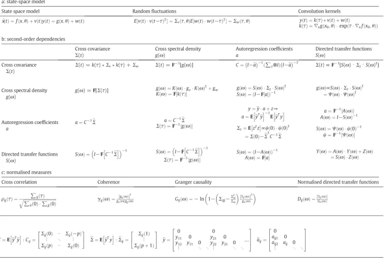
The purpose of this section is to clarify the straightforward relation-ships between spectral descriptions of data and the processes generating those data. This is important because if we know–or can estimate–the parameters of the generative process, then one can derive expected measures–such as cross-covariance functions, complex cross spectra, autoregressive coefﬁcients and directed transfer functions–analytically. In other words, measures that are typically used to characterise observed data can be regarded as samples from a probability distribution over Table 1

This table presents the expressions that relate unnormalised and normalised measures of second-order statistical dependencies among data to the underlying process generating those data. Table 1a specifies the generative (state-space) model in terms of stochastic differential equations of motion and a static nonlinear observer function. The randomfluctuations that perturb the motion of hidden (neuronal) states and the observation noise are characterised in terms of their second-order statistics; namely their covariance or spectral density. These state-space models can be formulated in terms of a convolution of thefluctuations, where the (first order Volterra) convolution kernels are a function of the model parameters. Table 1b shows how these kernels can generate any characterisation of the ensuing dependencies among the data–as cross-covariance functions of lag or time, cross spectral density functions of frequency and autoregressive formulations–in terms of autoregression coefficients and associated directed transfer functions. The expressions have been simplified and organised to illustrate the formal symmetry among the relationships. The key point to take from these expressions is that any characterisation can be derived analytically from any other using Fourier transformsF[·], expectationsE[·] convolution operators * and Kronecker tensor products⊗. Variables with a ~ denote matrices whose columns contain lagged func-tions of time and†denotes the conjugate transpose. Table 1c provides standardised versions of the second order statistics in Table 1b. These include the cross-correlation function, coher-ence, Geweke Granger causality and the normalised (Kaminski) directed transfer functions. These results mean that we can generate the expected Granger causality from the parameters of any generative model in exactly the same way that any other data feature can be generated. Note that in going from a parameterised generative model to the second-order statistics, there is no return. In other words, although second-order statistics can be generated given the model parameters, model parameters cannot be derived from second-order statistics. This is the (inverse) problem solved by DCM for complex cross spectra—that requires a generative model.

a: state-space model

State space model Randomﬂuctuations Convolution kernels

˙ x tð Þ ¼f xð;θÞ þv tð Þy tð Þ ¼g xð;θÞ þw tð Þ E½v tð Þ v t−ð τÞT_¼_Σ_v_ð_τ_;_θ_Þ_E_½_{w t}_{ð Þ}_{w t−}_ð _τ_ÞT_¼_Σ_w_ð_τ_;_θ_Þ y tð Þ ¼kð Þ τ v tð Þ þw tð Þ kð Þ ¼τ ∇xg xð0;θÞ expðτ∇xf xð0;θÞÞ b: second-order dependencies Cross covariance Σ(t)

Cross spectral density g(ω)

Autoregression coefﬁcients a

Directed transfer functions S(ω) Cross covariance Σ(t) Σ(t) =k(τ)∗Σv∗k(τ) +Σw Σ(t) =F−1[g(ω)] C¼ I−ea −1 ð∑z⊗IÞI−ea −T Σ(t)∝F−1_[_S_(ω)_⋅_Σ z⋅S(ω)†]

Cross spectral density g(ω) g(ω) =F[Σ(τ)] gð Þ ¼ω Kð Þ ω gvKð Þω†þgw Kð Þ ¼ω F½kð Þτ gð Þ ¼ω Sð Þ ω ΣzSð Þω † Sð Þ ¼ω ðI−F½ aÞ−1 gð Þω∝Sð Þ ω ΣzSð Þω† ¼Ψ ωð Þ Ψ ωð Þ† Autoregression coefﬁcients a a¼C−1e_Σ a¼C−1_Σe Σ τð Þ ¼F−1_½_g_{ð Þ}_ω y¼eyaþz⇒ a¼EheyTeyi−1EheyTyi Σz¼EzTz ∝ψð Þ 0 ψð Þ0† ¼Σð Þ0−ΣeTC−1_Σe a¼F−1_½_A_{ð Þ}_ω Að Þ ¼ω I−Sð Þω−1 Sð Þ ¼ω Ψ ωð Þ ψð Þ0−1 ψ¼F−1_½_{Ψ ω}_{ð Þ}

Directed transfer functions S(ω) Sð Þ ¼ω I−FhC−1_Σei−1 Sð Þ ¼ω I−FC−1Σe h i −1 Σ τð Þ ¼F−1_½_g_{ð Þ}_ω Sð Þ ¼ω ðI−Að ÞωÞ−1 Að Þ ¼ω F½ a Yð Þ ¼ω Að Þ ω Yð Þ þω Zð Þω ¼Sð Þ ω Zð Þω c: normalised measures

Cross correlation Coherence Granger causality Normalised directed transfer functions

ρijð Þ ¼τ ∑ijð Þτ ffiffiffiffiffiffiffiffiffiffiffiffiffiffiffiffiffiffiffiffiffiffiffiffiffiffiffiffiffiffiffiffiffi ∑iið Þ 0 ∑jjð Þ0 q γijð Þ ¼ω gijð Þω j j2 giið Þωgjjð Þω Gijð Þ ¼ω −ln 1− Σzjj− Σ2 zij Σzii Sijð Þω j j2 giið Þω Dijð Þ ¼ω Sijð Þω j j Siið Þω j j C¼EheyTeyi:Cij¼ Σijð Þ0 ⋯ Σijð−pÞ ⋮ ⋱ ⋮ Σijð Þp ⋯ Σijð Þ0 2 4 3 5 eΣ¼EheyTyi:Σeij¼ Σijð Þ1 ⋮ Σijðpþ1Þ 2 4 3 5 ey¼ 0 y11 0 y12 y11 0 ⋮ ⋱ ⋱ 0 y21 0 y22 y21 0 ⋮ ⋱ ⋱ … 2 6 6 4 3 7 7 5 eaij¼ 0 aij1 0 aij2 aij 0 ⋮ ⋱ ⋱ 2 6 6 4 3 7 7 5

(3)

functions, whose expectation is known. This means that one can examine the expected behaviour of normalised measures–like cross-correlation functions and spectral Granger causality_–as an explicit function of the parameters of the underlying generative process. We will use this fact to see how Granger causality behaves under different parameters of a neural mass model generating electrophysiological observations_—and different parameters of measurement noise.

In what follows, we usefunctional connectivityto denote a statistical dependence between two measurements andeffective connectivityto denote a causal inﬂuence among hidden (neuronal) states that produce functional connectivity. By deﬁnition, effective connectivity is directed, while directed functional connectivity appeals to constraints on the parameterisation of statistical dependencies that preclude non-causal dependencies. Because we will be discussing state-space and autoregressive formulations, we will also make a distinction between

fluctuationsthat drive hidden states andinnovations that underlie autoregressive dependencies among observations. Innovations are a fictive construct (effectively a mixture offluctuations and measurement noise) that induce an autoregressive form for statistical dependencies over time. Fourier transforms will be denoted byF[·], expectations by

E[·] convolution operators by * and Kronecker tensor products by⊗. Variables with a ~ denote (usually Toeplitz) matrices whose columns contain (lagged) functions of time and†means conjugate transpose.

Table 1a provides the basic form of the generative models that we will consider. This form is based on (stochastic and delay differential) equations of motion and a static mapping to observations. Any system of this sort has an equivalent Volterra series expansion that can be

summarised in terms of itsfirst order Volterra kernels. These kernels can be thought of as an impulse response to each source offluctuations. Table 1b shows how various measures of spectral power or variance (second-order statistics) can be derived from the kernels—and from each other. This table is arranged so that the representations of second-order statistics listed against the columns can be derived from the representations over the rows (see the glossary of variables that accompanies this table). For example, cross spectral density is the Fou-rier transform of the cross covariance function. The entries along the leading diagonal define the models of (linear) dependency upon which these characterisations are based. The odd and even columns pertain to functions of time and frequency respectively, where the Fourier transforms of the kernels are known as transfer functions, which we will refer to asmodulation transfer functionsto distinguish them fromdirected transfer functions(see below). The modulation transfer functions in turn specify the cross spectral density and the cross-covariance function. Note that deriving second-order measures from the (effective connectivity) parameters of the generative process is a one-way street. One cannot recover the parameters from the kernels

—in the sense that the mapping from parameters to kernels is not bijective (there are many combinations of parameters that produce the same kernels).

Second-order measures like cross-covariance and spectral density functions do not speak to directed functional connectivity because they do not appeal to any temporal precedence constraints—they simply reﬂect (non-causal) statistical dependence. In contrast, characterisations based upon autoregressive processes and causal

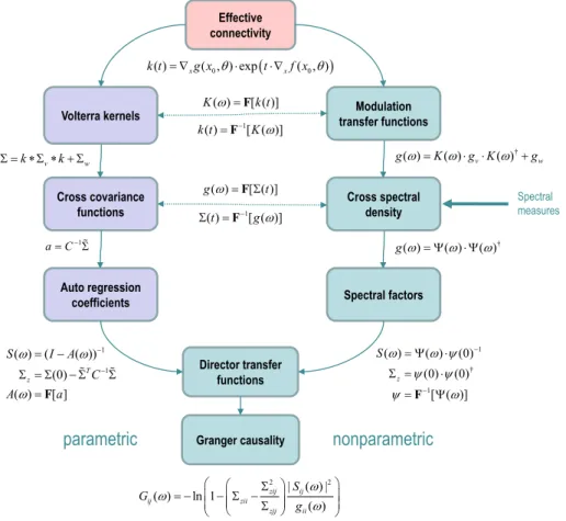
Fig. 1.This schematic illustrates the different routes one could take–using the equations inTable 1–to derive (spectral) Granger causality measures from the (effective connectivity) parameters of a model—or indeed empirical measures of cross spectral density. The key point made by this schematic is the distinction between parametric and nonparametric spectral causality measures. These both rest upon the proportion of variance explained, implicit in the directed transfer functions; however, in the parametric form, the transfer functions are based upon an autoregression model. In contrast, the nonparametric approach uses spectral matrix factorisation, under the constraint that the spectral factors are causal or minimum phase ﬁl-ters. The boxes in light green indicate spectral characterisations, while the light blue boxes indicate measures in the time domain. SeeTable 1and main text for a more detailed explanation of the variables and operators.

(4)

spectral factors are measures of directed statistical dependencies because they preclude non-causal influences. Autoregressive formulations do this by conditioning the current observation on previous observa-tions (but not future observaobserva-tions), while causal spectral factors corre-spond tofilters (transfer functions), whose Fourier transforms have zero values at future time points. These are also known as minimum phasefilters. Parametric Granger causality uses autoregressive formula-tions, while nonparametric measures are generally based on (Wilson–

Burg) spectral matrix factorisation (Dhamala et al., 2008; Nedungadi et al., 2009). Intuitively, this uses Newton's method tofind a square root (or factor) under the constraint that the Fourier transform of the factor is causal or a minimum phasefilter (Fomel et al., 2003). Once the cross spectral density has been factorised, the instantaneous part of the filter is removed —and becomes an estimate of the cross

covariance of the innovations. The expressions inTable 1b use standard linear algebra results based upon Wiener–Khinchin theorem, the Yule–

Walker relationships and (Wilson–Burg) spectral factorisation to show the relationships between different approaches to characterising second-order dependencies between time series.

Note above the difference between the modulation transfer function K(ω), the directed transfer functionS(ω) and the causal spectral factors

Ψ(ω). These all play similar roles asfilters or transfer functions but are distinct characterisations: the modulation transfer function is applied to the fluctuations to produce the observations, whereas the (unnormalised) directed transfer function is applied to the innovations. The directed transfer function only becomes the modulation transfer function–that mediates causal influences–in the absence of measure-ment noise. Finally, the causal spectral factors include both instantaneous Fig. 2.This schematic illustrates the state-space or dynamic causal model that we used to generate expected cross spectra and simulated data.Left panel: this shows the differential equa-tions governing the evolution of depolarisation in four populaequa-tions constituting a single electromagnetic source (of EEG, MEG or LFP measurements). These equaequa-tions are expressed in terms of second-order differential equations that can be rewritten as pairs offirst order equations, which describe postsynaptic currents and depolarisation in each population. These pop-ulations are divided into input cells in granular layers of the cortex, inhibitory interneurons and (superficial and deep) principal or pyramidal cell poppop-ulations that constitute the output populations. The equations of motion are based upon standard convolution models for synaptic transformations, while coupling among populations is mediated by a sigmoid function of (delayed) mean depolarisation. The slope of the sigmoid function corresponds to the intrinsic gain of each population. Intrinsic (within-source) connections couple the different popula-tions, while extrinsic (between-source) connections couple populations from different sources. The extrinsic influences (not shown) enter the equations in the same way as the intrinsic influences but in a laminar specific fashion (as shown in the right panel).Right panel: this shows the simple two source architecture used in the current paper. This comprises one lower source that sends forward connections to a higher source (but does not receive reciprocal backward connections). The intrinsic connectivity (dotted lines) and extrinsic connectivity (solid line) conform to the connectivity of the canonical microcircuit and the known laminar specificity of extrinsic connections (Bastos et al., 2012). Excitatory connections are in red and in-hibitory connections are in black. Randomfluctuations drive the input cells and measurements are based on the depolarisation of superficial pyramidal cells. SeeTable 2for a list of key parameters and a brief description.

Table 2

This table provides the parameter values used for simulations (and prior densities used for subsequent dynamic causal modelling). The left column describes the parameters (corresponding to the equations inFig. 2). The second column provides the values used to produce the spectra shown inFigs. 3 and 4. Theﬁnal two columns provide the prior mean and variance for dynamic causal modelling. Note that the variance is not the prior variance of the value per se but of its log scaling.

Description of parameter Parameter value used for simulations Prior mean Prior variance of log scaling Intrinsic connectionsdij(Hz) 45;…;15 1000 4 5;…;15 1000 1 8

Extrinsic connections (Hz) exp(2)⋅200 200 1

8 Rate constantsκi(Hz) 1₂;1₂;₁₆1;₂₈1 1000 1 2;12;161;281 1000 1 16

Slope of sigmoidγ exp1

8 23 23 321

Intrinsic delaysτ(ms) 1 1 1

32

Extrinsic delaysτ(ms) 4 8 1

32

Amplitude ofﬂuctuations exp(−2) 1 1

128

Exponent ofﬂuctuations 1 1 1

128

Amplitude of noise exp(−8) 1 1

128

Exponent of noise 1 1 1

(5)

inﬂuences and those embodied by directed transfer functions.Table 1c lists the normalised or standardised versions of non-causal (cross-covariance and spectral) and causal (directed transfer) functions. These are commonly used as the basis of inference about undirected and directed functional connectivity respectively (Friston et al., 2013).

Equipped with the expressions inTable 1, one can derive the expected functions that characterise functional connectivity, given the parameters of the underlying state-space model. Furthermore, one can derive any one representation from another. For example, starting from a parameterised state-space model, we can derive the Volterra kernels and resulting cross-covariance functions among observation channels. One can then compute the autoregressive coefﬁcients and directed transfer functions to compute parametric spectral Granger causality. Alternatively, one could take the Fourier transform of the kernels (and the cross-covariance functions of theﬂuctuations and measurement noise) to produce the expected cross spectrum over observed channels. Using spectral matrix factorisation, one can then identify the nonparametric directed transfer function and associated Granger causality. These two (parametric and nonparametric) routes are illustrated schematically inFig. 1.

To illustrate the derivation of expected transfer functions and Grang-er causality, we will use a standard state-space model from the suite of neural mass models used in the SPM software implementation of

dynamic causal modelling. This suite includes neural mass models based upon convolution operators (that model synaptic convolution of presynaptic inputs) or models that are nonlinear in the hidden states based upon conductance models (that model the interaction between voltage and transmembrane conductances). All of these neuronal mass models allow for the coupling of multiple sources, where each source comprises multiple neuronal populations (usually three or four).Fig. 2shows the canonical microcircuit neural mass model–a convolution model–that we will use in this paper. This particular model has been used previously to characterise things like intrinsic gain control mechanisms in hierarchical visual processing (Brown and Friston, 2012) and impaired top–down connectivity in minimally conscious states (Boly et al., 2011).

Because our focus is on spectral Granger causality, we limit ourselves to a simple bivariate case—with two channels reporting observed depolarisation in two sources. To examine the validity of expected causal measures, we consider the simplest case of a unidirectional (forward) connection from theﬁrst to the second source—that is not reciprocated. We wanted to see whether spectral Granger causality could properly discount the backward connections.Fig. 2details the architecture of this model, with four populations per source and one extrinsic forward connection between the sources. The intrinsic connec-tions couple different populaconnec-tions within a source—here, spiny stellate

Expected and estimated cross spectra

0 20 40 60 80 100 120 0 0.5 1 1.5 2 2.5 3x 10 -3 frequency density

Auto spectrum (first source)

0 20 40 60 80 100 120 0 1 2 3 4 5 6x 10 -4 frequency density

Cross spectral density

frequency

trial number

log auto spectra

20 40 60 80 100 120 2 4 6 8 10 12 14 16 frequency trial number

log cross spectra

20 40 60 80 100 120 2 4 6 8 10 12 14 16 Expected values AR(16) estimates Welch’s estimates

Fig. 3.Thisfigure illustrates the convergence of empirical estimates of spectral density av-eraged over multiple trials. The top row shows the absolute values of the auto (for thefirst source) and cross spectral density (between the two sources ofFig. 2). The red lines cor-respond to the expected spectra under the known parameters of the model (the parame-ters used for characterising spectral measures in subsequentfigures). The green and blue lines correspond to empirical estimates based upon 16 epochs of simulated (noisy) data, where each epoch comprised 1024 samples at a sampling rate of 256 Hz. The green lines report the estimates under an AR(16) model, while the blue lines used Welch's periodiogram method, as implemented in Matlab. Both give very similar results. The lower panels show the (absolute value) of the emerging average over 16 trials to show that stable estimates obtain after about eight trials—although many more are generally used in practice to obtain smooth spectral estimates.

Expected spectral Granger Causality

0 20 40 60 80 100 120 0 0.2 0.4 0.6 0.8 1 frequency density

first source

0 20 40 60 80 100 120 0 0.1 0.2 0.3 0.4 frequency density

backward

0 20 40 60 80 100 120 0 0.1 0.2 0.3 0.4 frequency density

forward

0 20 40 60 80 100 120 0 0.2 0.4 0.6 0.8 1 frequency density

second source

modulation transfer function directed transfer function Granger causality (parametric) Granger causality (non-parametric)

Fig. 4.Thisfigure reports the expected modulation transfer functions (blue lines), normal-ised directed transfer functions (green lines) and the associated spectral Granger causality (red lines: parametric—solid and nonparametric—dotted) under the dynamic causal model shown inFig. 1. In this example, measurement noise was suppressed (with log-amplitude of−8). The log-amplitude of the neuronalfluctuations was set at a fairly low level of−2. Thesefluctuations had a power law form with an exponent of one. The spec-tral measures are the expected values, given the model parameters, and correspond to what would be seen with a very large amount of data. Under these conditions, the (expect-ed) directed transfer functions and Granger causality identify the predominance of gamma in the forward connections—and correctly detect that there is no reciprocal or backward connection.

(6)

cells, inhibitory interneurons and superﬁcial and deep pyramidal cells. The equations in the boxes are the equations of motion that constitute the state-space model. Notice that these are delay differential equations because the sigmoid function of presynaptic input operates on the mean

depolarisation of the presynaptic source in the recent past—to accommodate axonal conduction delays. Intrinsic (within source) conduction delays are about 1 ms while extrinsic (between source) delays are about 4 to 8 ms.

We assumed that observed data were generated by the superﬁcial pyramidal cells, with parameterised measurement noise. The (neuro-nal)ﬂuctuations driving both the spiny stellate cells and the measure-ment noise had a 1/f or power law form. The amplitude of the measurement noise was suppressed to low values with a log scaling of−8. In other words, the spectral density of the measurement noise wasgw(ω) = exp(−8)⋅ω−1, where the frequencyωrange from one to 128 Hz. We used a sampling rate of 256 Hz or a sampling interval of about 4 ms. Using the parameters inTable 2, this pair of sources produces spectra of the sort shown inFig. 3. The expected spectra (red line) showed clear spectral peaks at beta and gamma frequencies superimposed on a power law form. The blue and green lines show the empirical estimates over 16 (1024 ms) epochs based on simulated data.Appendix Adescribes how the delay differential equations in Fig. 2were integrated.

Equipped with the expressions inTable 1, one can now derive the expected transfer functions and spectral Granger causality for any generative process speciﬁed in terms of its parameters.Fig. 4shows the functions expected using the parameters inTable 2. Note that the expected Granger causalities are not estimates—they are analytic reformulations of the underlying causal architecture using the expres-sions inTable 1. Given the (effective connectivity) parameters of the state-space model, the only thing that we have to specify is the order of the autoregressive model of linear dependencies (we used a model order ofp= 16 here and throughout).

The expected modulation (blue lines) and (normalised) directed transfer functions (green lines) report the shared variance between the two regions as a function of frequency. For these parameters, the causal spectral measures (directed transfer functions and Granger causality) properly identify the gamma peak and–more importantly–

assign all the causal effects to the forward connections—with no Granger causality in the backward direction. Note that the directed transfer functions are normalised and therefore have a different form to the modulation transfer functions. The modulation transfer functions report the total amount of power (at each frequency) in one source that appears in another. In short, under low level measurement noise, Granger causality can properly identify the directed functional connectivity in both qualitative and quantitative terms. In the next section, we explore the parameter space over which Granger causality retains its validity.

The effects of dynamical instability and measurement noise

We repeated the above analyses for different levels of some key parameters to illustrate two conditions under which Granger causality may fail. These parameters were the forward and backward extrinsic connection strengths, the intrinsic gain or the slope of the sigmoid function (Kiebel et al., 2007) and the amplitude of measurement noise (in the second source).Table 2lists the prior expectations for these parameters, whileFig. 5lists the levels we explored in terms of their log scaling.Fig. 5shows the results of these analyses in terms of (normalised) modulation transfer functions (green lines) and Granger causality (blue lines) associated with the forward (left panels) and backward connections (right panels). Pleasingly, when increasing forward connection strengths, Granger causality increases in proportion, without detecting any backward Granger causality. Similarly, when the backward effective connectivity was increased, Granger causality detect-ed this, while its estimate of forward influences remained unchanged. Interestingly, under these neural mass model parameters, the forward modulation transfer functions peak in the gamma range, while the backward connections peaked in the lower beta range. This is reminis-cent of physiologicalfindings: for example, recentfindings suggest that the superficial layers show neuronal synchronization and spike-field Fig. 5.Thisfigure reports the results of repeating the analysis of the previousfigure but

under different levels of various model parameters. The left column shows the estimates of forward connectivity in terms of the (normalised) modulation transfer function (green lines) and (parametric) spectral Granger causality estimates based upon an AR(16) process (blue lines). The modulation transfer functions were normalised according to Eq.(6)and can be regarded as the‘true’Granger causality. The right-hand columns show the equivalent results for the backward connection (which did not exist). Thefirst row shows the effects of increasing the extrinsic forward connection strengths. The ranges of parameters considered are shown as log scaling coefficients (in square brackets) of their expectation (shown below the range and inTable 2). The second, third and fourth rows report the results of similar changes to the backward connection strength, the intrinsic gain (slope of the sigmoid function inFig. 2) and the amplitude of measurement noise in the second channel. With these parameters, increases in forward connectivity amplify the coupling in the gamma range in the forward direction, while increases in backward ef-fective connectivity are expressed predominantly in the beta range. The key thing to note here is that changes in extrinsic connectivity are reflected in a veridical way by changes in spectral causality—detecting increases in backward connectivity when they are present and not when they are absent. However, Granger causality fails when intrinsic gain and measurement noise are increased—incorrectly detecting strong backward influences that peak in the gamma band high-frequency ranges.

(7)

coherence predominantly in the gamma frequencies, while deep layers prefer lower (alpha or beta) frequencies (Roopun et al., 2006, Maier et al., 2010; Buffalo et al., 2011). Since feedforward connections originate predominately from superﬁcial layers and backward connections from deep layers, this suggests that forward connections use relatively high frequencies, compared to backward connections (Bosman et al., 2012).

In contrast to changes in extrinsic connectivity, when intrinsic gain and measurement noise were increased, Granger causality fails in the sense that it detects strong and spectrally structured backward Granger causality. Interestingly, for increases in intrinsic gain, this spurious inﬂuence was localised to the gamma range of frequencies. In this example, the increase in measurement noise was restricted to the second channel and produced spurious spectral causality measures in high-frequency regimes. We now consider the reasons for these failures in terms of dynamical instability and measurement noise.

Dynamical instability

The failure of Granger causality with increasing intrinsic connectivity is used to illustrate a key point when modelling dynamical (biophysical) systems with autoregressive models. Autoregression processes model temporal dependencies among observations that are mediated by (long memory) dynamics of hidden states. One can express the dependencies between the current and past states as follows (using a local linear approximation):

∂x t_{ð Þ}

∂x tð−τÞ¼expðτ∇xfÞ 1

Clearly, if one wanted to model these dependencies with ap-th order autoregressive process, one would like the dependency above to be negligible whenτNp(wherepbecomes an interval of time). In other words, the eigenvaluesλof the Jacobian∇xfshould be sufﬁciently small to ensure that:

∂x tð Þ

∂x tð−pÞ≈0⇔expðp∇xfÞ ¼UexpðpλÞ U−≈0: 2

Here (U,U−) are the right and left eigenvectors of the Jacobian∇xf= U⋅λ⋅U−andλis a diagonal matrix containing eigenvalues—whose real parts are negative when the system is stable. This means that the autoregressive characterisation of temporal dependencies may be compromised by long range correlations of the sort associated with slowing near (transcritical) bifurcations. Note that transcritical slowing does not mean that_ﬂuctuations or oscillations slow down_—it means that modes of fast (e.g., gamma) activity decay slowly, where the rate of decay is determined by the real part of the largest eigenvalue (aka the Lyapunov exponent).

Practically, this suggests that if the (neuronal) system is operating near a transcritical bifurcation—and its eigenvalues approach zero from below, then the autoregressive formulation will not converge and associated spectral (Granger causality) measures become unreli-able. Technically, dynamical instability means that the covariance among observations becomes ill-conditioned, where the cross covari-ance (at zero lag) can be expressed in terms of the (real part of the) eigenvalues as follows: Σð Þ ¼0 −1₂∇xgU Reð Þλ− 1 U−ΣvU U−∇xg T þΣð Þ0w: 3

Eq.(3)means that the mode or pattern of activity described by the eigenvector whose eigenvalue approaches zero will decay much more slowly than the other modes and will dominate the cross-covariance. This is important because the auto regression coefﬁcients are computed using the inverse of the cross-covariance matrixa¼C−1_Σe_{. As the largest} (real) eigenvalue approaches zero, the inverse cross covariance matrix therefore becomes singular, precluding a unique solution for the autoregression coefﬁcients.

Based on this heuristic analysis, one might anticipate that the extrin-sic connectivity parameters do not increase the principal eigenvalue of the Jacobian (also known as the local Lyapunov exponent), whereas the intrinsic gain parameter does.Fig. 6(upper left panel) shows that increasing the intrinsic gain (expressed in terms of log scaling) produces eigenvalues with associated time constants of over 1/λ≥1/ 16 s—which exceeds the temporal support of an AR(16) model with 1/256 second time bins. The upper right panel shows the condition number (the ratio of the largest eigenvalue to the smallest) of the cross-covariance matrix, where a larger condition number indicates a (nearly) singular matrix. The lower panels ofFig. 6illustrate the ensuing failure of an autoregressive characterisation of spectral responses by comparing the expected spectrum (from thefirst source) with the autoregressive approximation associated with the coefficients derived Fig. 6.Thisfigure shows why Granger causality based upon (finite-order) autoregressive

processes fail under increasing intrinsic gain (and any other parameter that induces insta-bility through a transcritical bifurcations).Upper left panel: this show the principal (largest real part of the) eigenvalue of the systems Jacobian; also known as the Lyapunov expo-nent. When this eigenvalue approaches zero from below, perturbations of the associated eigenfunction of hidden states decay very slowly—and become unstable when the eigen-value becomes positive. One can see that increasing the intrinsic gain (red line) induces a transcritical bifurcation at about a log scaling of one. Furthermore, at a log scaling of .8, the time constant associated with the eigenvalue becomes greater thanpΔt¼16

256¼161 sec-onds (dashed line). The blue and green lines show the equivalent results as the (forward and backward) extrinsic connectivity is increased—showing no effect on the eigenvalue. However, increasing the intrinsic delay induces instability and critical slowing. This causes the condition number of the cross covariance matrix to increase, where a large condition number indicates a matrix is (nearly) singular or rank efficient.Upper right panel: this shows the corresponding condition number of the cross covariance matrix used to com-pute the autoregression coefficients, using the same format as the previous panel.Lower left panel: this shows the corresponding (log) spectral density (of thefirst source) over the same range of intrinsic gains shown in the upper panel. It shows that the beta and gamma peaks increase in frequency and amplitude with intrinsic gain.Lower right panel: this shows the difference between the expected auto spectrum (shown on the right) and the approximation based upon autoregression coefficients estimated using the associ-ated cross-covariance functions. It can be seen that these differences become marked when the condition number exceeds about 10,000.

(8)

analytically from the expected cross-covariance function. One can see that marked differences are evident when the condition number of the cross covariance matrix exceeds about 10,000. Clearly, one could consider increasing the order of the autoregressive process; however, when the cross covariance matrix becomes (nearly) singular, one would need a (nearly) inﬁnite order process.

Other model parameters that cause the principal eigenvalue to approach zero from below include the intrinsic and extrinsic delays (seeFig. 6). This is important, because neuronal systems necessarily have delays, which effectively increases the number of hidden states to inﬁnity: strictly speaking, the introduction of delays into the system's characteristic function induces an inﬁnite number of eigenvalues (Driver, 1977). This (almost) inevitably produces near zero Lyapunov exponents and is an important source of critical behaviour in biological systems (Jirsa and Ding, 2004). Another perspective on the failure of autoregressive formulations is based on the fact that a (linear) state-space model withmhidden states has an AR(p) formulation, wherem= 2p(Nalatore et al., 2007). When the number of effective

states increases to infinity, the associated infinite-order AR process cannot be approximated with afinite-order autoregressive process.

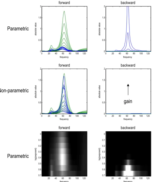
One remedy for systems that show critical behaviour is to abandon thefinite-order autoregressive formulation and consider nonparametric estimates of Granger causality based on spectral matrix factorisation (Nedungadi et al., 2009).Fig. 7takes a closer look at the effect of increas-ing intrinsic gain and compares the performance of autoregressive and Wilson–Burg spectral causality measures. As one might predict, the Wilson–Burg estimatesfinesse the problem of unstable modes and may therefore be preferable in the characterisation of neuronal timeseries. Heuristically, the Wilson–Burg estimates can do this because they have more degrees of freedom to model (minimum phase) linear dependen-cies. In other words, minimum phasefilters require more numbers to specify them than the number of coefficients available to AR models of the order used. Clearly, this latitude introduces a potential trade-off in terms of overfitting; however, in this setting Wilson–Burg procedures provide better estimates of the true (expected) Granger causality (green lines inFig. 7).

Fig. 7.Thisﬁgure presents a more detailed analysis of the effects of increasing intrinsic gain on spectral Granger causality measures. The left column shows the (normalised) modulation transfer function (green line) and Granger causality (blue line) over eight (log) scaling values of intrinsic connectivity. The right panels show the equivalent results for the backward connection. The top row shows the expected parametric Granger estimates based upon an autoregressive process, while the middle row shows the equivalent results for the expected nonparametric measure. The lower row shows the same results as in the upper row but in image format (with arbitrary colour scaling) to clarify the effects of increasing intrinsic gain. The key thing to take from these results is that parametric Granger causality is unable to model the long-range correlations induced by dynamical instability and, improperly, infers a strong backward connectivity in a limited gamma range. In contrast, the nonparametric measure is not constrained to model autoregressive dependencies and properly reﬂects the increase in forward coupling—without reporting any backward coupling.

(9)

Measurement noise

The failure of Granger causality in the context of measurement noise is slightly more problematic. This failure is almost self-evident from the relationship between the modulation transfer function and the directed transfer function. FromTable 1:

gð Þ ¼ω Kð Þ ω gvð Þ ω Kð Þω†þgwð Þω∝Sð Þ ω ΣzSð Þω†: 4

This expression says that the observed spectral density can be decomposed into measurement noise and shared variance mediated by (neuronal) ﬂuctuations. It is the latter that underlies spectral measures of directed functional connectivity—and not the former. We therefore require the directed transfer functions to be proportional to the modulation transfer functions

Kð Þ ω gvð Þ ω Kð Þω†∝Sð Þ ω ΣzSð Þω†: 5

In this case, the (off-diagonal terms of the) normalised directed transfer functions report the shared variance. This constraint portends some good news and some bad news: the good news is that there is

no requirement that the spectral power of the innovations has to be the same for all frequencies (this is why the covariance of the innovations

Σz∝gz(ω) is used as a proxy for their spectral density inTable 1—and why some equalities are proportionalities). This means that normalised spectral measures–like directed transfer functions and Granger causality–do not have to assume the innovations are white. In other words, they can cope with serially correlated innovationsgz(ω) of the sort we have used for the underlyingﬂuctuationsgv(ω).

The bad news is that for the proportionality above to hold the measurement noise has to be negligible (or proportional to the shared component). This is a simple but fundamental observation, which means that Granger causality can become an unreliable measure in the presence of substantial measurement noise. This problem was identiﬁed nearly half a century ago (Newbold, 1978) and has recently started to attract serious attention: see (Nalatore et al., 2007) for a comprehensive deconstruction of the problem in the context of autoregressive formulations. See alsoSolo (2007)who consider the effects of measurement noise under AR models and conclude that

“state space or vector ARMA models are needed instead.”

In brief, we can summarise the situation as follows: the spectral causality we seek is mediated by the modulation transfer functions. Fig. 8.Thisfigure uses the same format as in the previousfigure; however here, we have increased the amplitude of measurement noise (from a log amplitude−8 to−2). This measurement noise had channel-specific and shared components at a log ratio of one (i.e., a ratio of about 2.72). At nontrivial levels of noise (with a log-amplitude of about−4) the expected Granger causality fails for both parametric and nonparametric measures. The predominant failure is a spurious reduction in the forward spectral causality and the emergence of low-frequency backward spectral causality with nonparametric measures. The inset on the upper right shows the impact of noise on the coherence between the two channels at low (solid) and high (dotted) levels of noise.

(10)

These modulation transfer functions can be approximated by directed transfer functions when measurement noise can be ignored. In this case, the_fluctuations and innovations become the same. Furthermore, if we make the simplifying assumption that the spectral profile of thefl uctua-tions (and implicitly the innovauctua-tions) is the same for all sources, we can re-place their cross spectral density with their covariance. This can be expressed formally to recover the conventional expression for spectral Granger causality: Gijð Þ ¼ω −ln 1− gvjjð Þω− gvijð Þω 2 g_viið Þω 0 B @ 1 C AKijð Þω 2 K_iið Þω 0 B @ 1 C A ¼−ln 1− g_zjjð Þω−gzijð Þω 2 g_ziið Þω 0 B @ 1 C ASijð Þω 2 S_iið Þω 0 B @ 1 C A wheng_wð Þ ¼ω 0:∀ω ¼−ln 1− Σzjj− Σ2 zij Σzii !_S ijð Þω 2 giið Þω 0 B @ 1 C A wheng_wð Þ ¼ω 0 andg_vð Þω∝Σz:∀ω: 6

Fig. 8shows what happens when measurement noise cannot be ignored by increasing its log-amplitude from trivial values (of−8) to the level of the_fluctuations. Here, we increased both the power of the measurement noise that was shared and unique to each channel (where the shared component was smaller than the unique component by a log-amplitude of one). This simulates a range of signal-to-noise ratios from almost negligible to very high levels. This can be seen in the inset ofFig. 8, which shows the coherence between the two channels for the eight noise levels considered. For thefirst four levels, nearly all the coherence is mediated by neuronalfluctuations; whereas at the last level of measurement, noise dominates the coherence (through the shared component).

The effect of noise, as one might intuit, starts to emerge when the noise is no longer trivial in relation to signal—here at about a log-amplitude of−4. At this point, the Granger causal measures of forward connectivity start to fall and nontrivial backward connectivity emerges. Interestingly, in the nonparametric case, the spurious spectral coupling is in the same (low-frequency)

DCM-GC

DCM fits to CSD

0 128 100 200 -1 0 1 2 3 4 5 6 7 8

Frequency (Hz) and time (ms)

real

prediction and response (real)

0 128 100 200 -0.4 -0.3 -0.2 -0.1 0 0.1 0.2 0.3 0.4 imaginary

prediction and response (imaginary)

Frequency (Hz) and time (ms)

modulation transfer function Granger causality (true) Granger causality (source) Granger causality (channel)

0 20 40 60 80 100 120 0 0.2 0.4 0.6 0.8 frequency density first source 0 20 40 60 80 100 120 0 0.02 0.04 0.06 0.08 0.1 frequency density backward 0 20 40 60 80 100 120 0 0.05 0.1 0.15 0.2 0.25 0.3 0.35 frequency density forward 0 20 40 60 80 100 120 0 0.2 0.4 0.6 0.8 frequency density second source

Fig. 9.Thisfigure reports the results of a Granger causality analysis thatfinesses the measurement noise problem by basing spectral causality measures on the parameters estimated by dynamic causal modelling:Left panel: these plots show the observed (full lines) and predicted (dotted lines) cross spectra, in terms of real (upper panel) and imaginary (lower panel) parts. In most regimes, thefit is almost perfect; however, there are some small prediction errors around 20 Hz in the imaginary part. Thefirst portion of these predicted and observed profiles corresponds to the spectra, while the last portion is the (real) cross-covariance function. Both of these data features are used to improve the convergence of model inversion.Right panel: this shows the results of Granger causality measures based upon DCM using the format ofFig. 4. In this instance, the modulation transfer function is a maximum a posteriori estimate (dotted line). The solid blue line is the normalised modulation transfer function based on the true parameter values and can be regarded as the true Granger causality (see Eq.(6)). Crucially, the Granger causality among the sources (red line) correctly reports the absence of any backward coupling and is almost identical to the true Granger causality. Contrast this with the naive Granger causality (green line) based on observed responses with measurement noise. Here, the backward Granger causality attains nontrivial levels at low frequencies that are not present.

(11)

ranges for both forward and backward connections. One might suppose that this is a reﬂection of the symmetrical cross spectral density induced by noise.

It should be emphasised that the levels of noise that impact on spectral causality measures are large in relation to typical electro-physiological recordings, especially LFP recordings. In typical data analysis situations, one should be able to diagnose recordings with high levels of shared measurement noise using measures that are sensitive to non-causal shared variance (e.g., volume conduction), like imaginary coherence and the weighted phase-locking index (Nolte et al., 2004; Vinck et al., 2012). In these situations, it is well-known that Granger causal analysis can be confounded (Nalatore et al., 2007). In the next section, we explore how DCM can mitigate this problem.

In summary, the naive application of Granger causality to measured data is unreliable unless the measurements are relatively noiseless. This observation speaks to the fundamental difference between approaches that try to characterise dependencies among observations and approaches that acknowledge observations are generated by hidden states, such as dynamic causal modelling. Does this mean that spectral Granger causality should be abandoned in the setting of noisy measure-ments? Not necessarily. In theﬁnal section, we consider how valid Granger causality estimates can be recovered from dynamic causal modelling.

Dynamic causal modelling of Granger causality

In the previous section, we saw that nonparametric Granger causality _ﬁnesses the problems associated with characterising biological timeseries generated by coupled and delayed dynamics with unstable (slow) modes of behaviour. However, nonparametric Granger causality fails in the presence of measurement noise. Here, we provide a proof of principle that the problem of measurement noise can be dissolved by computing the Granger causality based upon the modulation transfer functions estimated by dynamic causal modelling (see Eq.(6)).

Put simply, using an explicit model of (realistic)fluctuations and measurement noise, one can estimate the Granger causality that would have been seen in the absence of noise. This is illustrated in Fig. 9, where we have inverted a model of the generative process using standard (variational Laplace) procedures (Friston et al., 2007) to estimate the effective connectivity parameters. These parameters provide the modulation transfer functions—and the corresponding Granger causality measures that properly reflect the spectral structure of forward in_fluences and the absence of backward connectivity. In this example, wefitted the expected cross spectra in channel space using the (known) form of the neural mass model with (unknown) parameters and the usual priors for this model (provided inTable 2).

For those people not familiar with dynamic causal modelling, DCM is a Bayesian model comparison and inversion framework for state-space models formulated in continuous time. It uses standard variational Bayesian procedures toﬁt timeseries or cross spectra–

under model complexity constraints – to provide maximum a posteriori estimates of the underlying (effective connectivity) model parameters. SeeFriston et al. (2012)for more details in this particular setting. This iterative procedure usually converges within about 32 iterations, producing the sort of_ﬁts shown in the left panels ofFig. 9. In short, DCM solves the inverse problem of recovering plausible parameters (of both neuronal dynamics and noise) that explain observed cross spectra.

In summary, provided that one can solve the inverse problem posed by dynamic causal modelling, one can recover veridical Granger causality measures in the spectral domain. Crucially, this requires accurate models of the underlying generative process. From the point of view of dynamic causal modelling, these measures

provide an intuitive and quantitative report of the directed frequency-specific influences mediated by effective connectivity. Speci_fically, they are the normalised modulation transfer functions (as opposed to the normalised directed transfer functions). From the point of view of spectral Granger causality, DCM has just been used to place constraints on the parametric form of the underlying dynamics, which enable observed power to be partitioned into signal (generated by hidden states) and noise.

Conclusion

In conclusion, we have shown that naïve Granger causality is not appropriate for noisy measurements of coupled dynamical systems with delays. Having said this, it is fairly straightforward to compute Granger causality measures of directed functional connectivity from estimates of directed effective connectivity_—as provided by dynamic causal modelling. In their analysis of measurement noise,Nalatore et al. (2007)proposed a solution based upon a linear state-space model and Bayesian model inversion (an expectation maximisation scheme based upon Kalman smoothing). The same approach–to estimating measurement noise by modelling dependencies with linear state-space models–appears to have been proposed independently bySommerlade et al. (2012). Although this approach may fail when the process generating data exhibits critical dynamics, it nicely highlights the need to explicitly model hidden states generating observed data—such that covariance induced byﬂuctuations in hidden states can be separated from covariance due to measurement noise; see alsoRobinson et al. (2004). In short, a failure to model hidden states may produce false inferences when naïvely applying spectral Granger causality to observed data.

This conclusion shifts the problem from worrying about the shortcomings of Granger causality to worrying about the problems posed by dynamic causal modelling. These problems should not be underemphasised (Daunizeau et al., 2011): in the illustration above, we used a dynamic causal model that had the same form as the process generating noisy observations. Clearly, this model will not be known in real world applications. This means that the DCM has to be optimised in relation to the data at hand—using Bayesian model comparison or averaging (Penny et al., 2004). This speaks to an open issue in DCM; namely, how to score and invert alternative models of observed data in an accurate and efﬁcient fashion. In one sense, this problem is the focus of nearly all current work on dynamic causal modelling and_– al-though much progress has been made–dynamic causal modelling is still in its infancy. This model optimisation speaks to the continuous process of perfecting the underlying model of neuronal dynamics as more information about neuronal circuits becomes available. This is at the heart of a Bayesian approach to data modelling: placing knowledge in the model to provide more informed constraints and better estimates of causal interactions.

We have distinguished between estimates of Granger spectral causality based upon autoregressive processes and spectral factorisation as parametric and nonparametric respectively (Dhamala et al., 2008). For some people, this is contentious because both rest upon models of statistical dependencies that have implicit parameters. For example, the autoregression coefficients in autoregressive models or the minimum phasefilters produced by spectral factorisation. In this sense, both are parametric. Conversely, unlike dynamic causal modelling, neither parametric nor nonpara-metric Granger causality are equipped with parameterised models of how dependencies are generated. In this sense, they are both nonparametric. The slightly unfortunate use of parametric and nonparametric could befinessed by explicit reference to the underlying model of dependencies; e.g., autoregressive or minimum phase (as suggested by our reviewers).

It is well-known that long-range temporal autocorrelations are problematic for Granger causality. Non-invertible (even if causal)

(12)

ﬁltering can induce such autocorrelations; as will long-memory processes (e.g. power–law autocorrelation decay found in fractionally-integrated autoregressive processes). Granger causality is not well-deﬁned for such processes because they do not satisfy prerequisite spectral conditions (Geweke, 1982). We have consid-ered this issue in terms of dynamical instability in the vicinity of transcritical bifurcations—when the system's principal Lyapunov exponent (real eigenvalue) approaches zero from below. In spectral theory, this instability can be characterised in terms of thespectral radius; which is the largest (supremum) over a system's spectrum of absolute eigenvalues. A recent discussion of these issues can be found inBarnett and Seth (2014).

The focus of this technical note has been rather pragmatic: it has focused on the technical issue of estimating Granger causality in the presence of measurement noise and long range correlations. Fur-thermore, we have restricted our treatment to spectral measures of Granger causality. One might ask why measure Granger causality with dynamic causal modelling if one has already estimated the causal in_ﬂuences (effective connectivity and associated transfer functions) en route. In the setting of effective and functional connec-tivity, Granger causality has been cast as a measure of directed func-tional connectivity (Friston et al., 2013). Given that functional connectivity is a measure of statistical dependencies or mutual infor-mation, this means that Granger causality measures the directed mutual information between the present state (of a target) and the past state (of a source). Formally, directed mutual information corre-sponds to transfer entropy (Lindner et al., 2011). This is important because there is equivalence between Granger causality and transfer entropy (Barnett et al., 2009), which therefore allows one to quantify directed information transfer in terms of Granger causal estimates. This suggests that it is possible to relate causal inﬂuences (effective connections) to their information theoretic consequences in a quantitative sense.

Finally, we have not addressed how to assess the signiﬁcance of Granger causality. Generally, this would proceed using some form of nonparametric inference based upon (surrogate) data in which directed temporal dependencies are destroyed. Although our focus has been on estimation, as opposed to inference, it is worth noting that–from the perspective of DCM–inference rests on comparing the evidence for models generating Granger causality metrics. In other words, one would ﬁrst select the DCM with the highest model evidence, after which Granger causal measures would be used to characterise directed functional connectivity in a quantita-tive fashion.

Acknowledgments

KJF is funded by a Wellcome Trust Principal Research Fellowship (Ref: 088130/Z/09/Z). We would like to thank our reviewers for careful and detailed help in presenting this work.

Software note: the graphics and simulations reported in this paper can be reproduced using the academic freeware available from:http:// www.ﬁl.ion.ucl.ac.uk/spm/. These simulations are accessed through the graphical user interface of theNeural_demoToolbox (‘Granger causality’). This demonstration routine calls on routines in the spectral Toolbox that implement the transformations inTable 1. These include: spm_ccf2gew.m, spm_ccf2mar.m, spm_csd2ccf.m, spm_mar2ccf.m, spm_csd2coh.m, spm_mar2csd.m, spm_csd2gew.m, spm_csd2mar.m, spm_ccf2csd.mandspm_dtf2gew.m.

Appendix A

This appendix describes the integration of delay differential equa-tions using a high order Taylor expansion in generalised coordinates of motion. This scheme was used to generate the simulated timeseries and their expected cross spectra shown inFig. 3—and to evaluate the

Jacobian and associated transfer functions that determine the expected Granger causality in subsequent analyses. The Jacobian depends sensi-tively on delays as described below.

Consider the problem of integrating (solving) the set of delay differ-ential equations whereτijis the (asymmetric) delay from statejtoi

˙ xið Þ ¼t X jfi xj t−τij : A:1

Using a local linear approximation and Taylor's theorem, we have

˙ xið Þ ¼t X j ∂fi ∂xj xj t−τij ¼X_j∂fi ∂xj xjð Þ þt x˙jð Þt −τij þ1₂xjð Þt −τij 2 þ… : A:2 This can be expressed more compactly in matrix form usingJ=∇xf (evaluated at the current state orﬁxed point) and the Hadamard product ×:

˙

x¼JxþðJð−τÞÞx˙þ1₂ðJð−τÞ ð−τÞÞxþ… A:3 If we now assume the existence of a (ﬁrst-order) approximation of Eq.(A.3)with the formx˙≈Qx, then substitution into Eq.(A.3)gives

˙

x≈JxþðJð−τÞÞQxþ1₂ðJð−τÞ ð−τÞÞQ2xþ… A:4 This means that the (approximate) Jacobian we seek is the solution to the matrix polynomial:

Q¼JþðJð−τÞÞQþ1₂ðJð−τÞ ð−τÞÞQ2þ… A:5

This polynomial can be solved reasonably efﬁciently using the Robbins Monro algorithm as follows (using a suitably largeNthat en-sures convergence of the Taylor expansion).

Qiþ1¼ 1 2Qiþ 1 2 XN n¼0 1 n!ðJð−τÞ ð−τÞ …ð−τÞÞQ n i: A:6

The algorithm can be initialised with the solution to theﬁrst-order approximation to Eq.(A.5)(this approximation is used directly for simpler neural mass models):

Qo¼J−ðJτÞQo

¼ðIþJτÞ−1

J: A:7

This scheme appears to give good approximations when checked numerically.

(13)

References

Barnett, L., Seth, A., 2014.The MVGC multivariate Granger causality toolbox: a new approach to Granger-causal inference. J. Neurosci. Methods 223, 50–68.

Barnett, L., Barrett, A., Seth, A., 2009.Granger causality and transfer entropy are equivalent for Gaussian variables. Phys. Rev. Lett. 103 (23), 238701.

Bastos, A.M., Usrey, W.M., Adams, R.A., Mangun, G.R., Fries, P., Friston, K.J., 2012.Canonical microcircuits for predictive coding. Neuron 76 (4), 695–711.

Boly, M., Garrido, M.I., Gosseries, O., Bruno, M.A., Boveroux, P., Schnakers, C., Massimini, M., Litvak, V., Laureys, S., Friston, K., 2011.Preserved feedforward but impaired top–down processes in the vegetative state. Science 332 (6031), 858–862. Bosman, C.A., Schoffelen, J.-M., Brunet, N., Oostenveld, R., Bastos, A.M., Womelsdorf, T.,

Rubehn, B., Stieglitz, T., De Weerd, P., Fries, P., 2012.Attentional Stimulus Selection through Selective Synchronization between Monkey Visual Areas. Neuron. 75, 875–888.

Brown, H.R., Friston, K.J., 2012.Dynamic causal modelling of precision and synaptic gain in visual perception—an EEG study. Neuroimage 63 (1), 223–231.

Buffalo, E.A., Fries, P., Landman, R., Buschman, T.J., Desimone, R., 2011.Laminar differences in gamma and alpha coherence in the ventral stream. Proc. Natl. Acad. Sci. 108, 11262.

Bullmore, E., Long, C., Suckling, J., Fadili, J., Calvert, G., Zelaya, F., Carpenter, T.A., Brammer, M., 2001.Colored noise and computational inference in neurophysiological (fMRI) time series analysis: resampling methods in time and wavelet domains. Hum. Brain Mapp. 12 (2), 61–78.

Daunizeau, J., David, O., Stephan, K.E., 2011.Dynamic causal modelling: a critical review of the biophysical and statistical foundations. Neuroimage 58 (2), 312–322. David, O., Kiebel, S., Harrison, L., Mattout, J., Kilner, J.M., Friston, K.J., 2006.Dynamic causal

modeling of evoked responses in EEG and MEG. Neuroimage 30, 1255–1272. Dhamala, M., Rangarajan, G., Ding, M., 2008.Analyzing informationﬂow in brain

networks with nonparametric Granger causality. Neuroimage 41 (2), 354–362. Driver, R.D., 1977.Ordinary and Delay Differential Equations. Springer Verlag, New York. Fomel, S., Sava, P., James Rickett, J., Claerbout, J.F., 2003.The Wilson–Burg method of spec-tral factorization with application to helicalﬁltering. Geophys. Prospect. 51, 409–420. Friston, K., Mattout, J., Trujillo-Barreto, N., Ashburner, J., Penny, W., 2007.Variational free

energy and the Laplace approximation. Neuroimage 34 (1), 220–234.

Friston, K.J., Bastos, A., Litvak, V., Stephan, E.K., Fries, P., Moran, R.J., 2012.DCM for complex-valued data: cross-spectra, coherence and phase-delays. Neuroimage 59 (1), 439–455.

Friston, K., Moran, R., Seth, A.K., 2013.Analysing connectivity with Granger causality and dynamic causal modelling. Curr. Opin. Neurobiol. 23 (2), 172–178.

Geweke, J., 1982.Measurement of linear dependence and feedback between multiple time series. J. Am. Stat. Assoc. 77, 304–313.

Granger, C.W.J., 1969.Investigating causal relations by econometric models and cross-spectral method. Econometrica 37, 424–438.

Jirsa, V.K., Ding, M., 2004.Will a large complex system with time delays be stable? Phys. Rev. Lett. 93 (7), 070602.

Kiebel, S.J., Garrido, M.I., Friston, K.J., 2007.Dynamic causal modelling of evoked responses: the role of intrinsic connections. Neuroimage 36 (2), 332–345. Lindner, M., Vicente, R., Priesemann, V., Wibral, M., 2011.TRENTOOL: a Matlab open

source toolbox to analyse informationﬂow in time series data with transfer entropy. BMC Neurosci. 12, 119.

Maier, A., Adams, G.K., Aura, C., Leopold, D.A., 2010. Distinct superﬁcial and deep laminar domains of activity in the visual cortex during rest and stimulation. Front. Syst. Neurosci. 4, 31.http://dx.doi.org/10.3389/fnsys.2010.00031.

Moran, R.J., Stephan, K.E., Kiebel, S.J., Rombach, N., OConnor, W.T., Murphy, K.J., Reilly, R.B., Friston, K.J., 2008.Bayesian estimation of synaptic physiology from the spectral responses of neural masses. Neuroimage 42 (1), 272–284.

Nalatore, H., Ding, M., Rangarajan, G., 2007.Mitigating the effects of measurement noise on Granger causality. Phys. Rev. E Stat. Nonlinear Soft Matter Phys. 75 (3 Pt 1), 031123.

Nedungadi, A.G., Rangarajan, G., Jain, N., Ding, M., 2009.Analyzing multiple spike trains with nonparametric Granger causality. J. Comput. Neurosci. 27 (1), 55–64. Newbold, P., 1978.Feedback induced by measurement errors. Int. Econ. Rev. 19, 787–791. Nolte, G., Holroyd, T., Carver, F., Coppola, R., Hallett, M., 2004.Localizing brain interactions

from rhythmic EEG/MEG data. Conf. Proc. IEEE Eng. Med. Biol. Soc. 2, 998–1001. Penny, W.D., Stephan, K.E., Mechelli, A., Friston, K.J., 2004.Comparing dynamic causal

models. Neuroimage 22 (3), 1157–1172.

Robinson, P.A., Rennie, C.J., Rowe, D.L., OConnor, S.C., 2004.Estimation of multiscale neu-rophysiologic parameters by electroencephalographic means. Hum. Brain Mapp. 23 (1), 53–72.

Roopun, A.K., Middleton, S.J., Cunningham, M.O., LeBeau, F.E., Bibbig, A., Whittington, M.A., Traub, R.D., 2006.A beta2-frequency (20–30 Hz) oscillation in nonsynaptic networks of somatosensory cortex. Proceedings of the National Academy of Sciences 103, 15646.

Shin, C.W., Kim, S., 2006.Self-organized criticality and scale-free properties in emergent func-tional neural networks. Phys. Rev. E Stat. Nonlinear Soft Matter Phys. 74 (4 Pt 2), 45101. Solo, V., 2007.On causality I: sampling and noise. Proc. 46th IEEE Conference on Decision

and Control, New Orleans.

Sommerlade, L., Thiel, M., Platt, B., Plano, A., Riedel, G., Grebogi, C., Timmer, J., Schelter, B., 2012.Inference of Granger causal time-dependent inﬂuences in noisy multivariate time series. J. Neurosci. Methods 203 (1), 173–185.

Stam, C.J., de Bruin, E.A., 2004.Scale-free dynamics of global functional connectivity in the human brain. Hum. Brain Mapp. 22 (2), 97–109.

Vinck, M., Battaglia, F.P., Womelsdorf, T., Pennartz, C., 2012.Improved measures of phase-coupling between spikes and the Local Field Potential. J. Comput. Neurosci. 33 (1), 53–75 (Aug).

Variable Description

x(t) Hidden states of a state-space or dynamic causal model

y(t) Observed measurements or response variable

f(x,θ) Nonlinear equations of motion orﬂow

g(x,θ) Nonlinear observation or measurement equation

v(t) Randomﬂuctuations in the motion of hidden states

w(t) Random measurement noise

z(t) Innovations of an autoregressive model

Σv(τ,θ) Covariance function ofﬂuctuations

Σw(τ,θ) Covariance function of noise

Σz∝ψ(0)⋅ψ(0)* Covariance matrix of innovations

∇xf Jacobian or gradient ofﬂow with respect to hidden states