ESCUELA TÉCNICA SUPERIOR DE INGENIERÍA
INFORMÁTICA
GRADO EN INGENIERIA DEL SOFTWARE
Acercamiento multi-objetivo para la minimización de casos
de prueba en Líneas de Producción de Software.
Multiobjective approaches for the minimization of test suites
in Software Product Lines.
Realizado por
Javier Norberto Alarcón Jaén
Tutorizado por
Gabriel Jesús Luque Polo
Departamento
Lenguajes y Ciencias de la Computación
UNIVERSIDAD DE MÁLAGA MÁLAGA, Octubre 2015
Resumen
En la actualidad muchos desarrollos están guiados por los clientes, y por ello, la mayoría de las empresas se dirigen a las necesidades de sus clientes potenciales mediante la creación de una línea de productos -un portfolio de productos estrechamente relacionados con las variaciones en las características y funciones- en lugar de sólo un único producto. Las herramientas y técnicas para el desarrollo habituales de software tienden a centrarse productos individuales y este tipo de desarrollo de múltiples productos entrelazados es compleja.
El objetivo principal de este proyecto es desarrollar una estrategia de optimización para poder abordar el problema planteado previamente y que nos permita reducir el número de casos de prueba a aplicar en un tiempo razonable pero que a la vez se mantenga la calidad de los productos software resultantes. Para esto usaremos diferentes técnicas multi-objetivos y mono-objetivos y haremos comparación de los resultados obtenidos.
Palabras claves
Optimización, multiobjetivo, algoritmos genéticos, búsqueda aleatoria, frente de Pareto, líneas de producción software, casos de prueba.
Abstract
Currently many developments are guided by customers, and therefore, most companies focus on the needs of their potential customers by creating a software product line -a portfolio of products closely related to variations in features and functions- rather than just a single product. The tools and techniques for the common development of software tend to focus individual products and development, of such multiple and interrelated products, is complex.
The main objective of this project is develop an optimization strategy to dealt with the previous problem and it allows us to reduce the number of test cases to apply in a reasonable time, but maintaining the quality of the resulting software products. Finally, we compare results using several different algorithms (mono-objective and multi-(mono-objectives approaches).
Keywords
Optimization, multi-objective, GA (genetic algorithm), random search, Pareto front, software product lines, test cases.
Index
Resumen ... 5
1. Introduction ... 9
1.1 Methodology ... 10
1.2 Organization of This Document ... 10
2. Background Information ... 13 2.1 Combinatorial Optimization ... 13 2.1.1 Multi-objective Optimization ... 13 2.1.1 Mono-objectivization Techniques ... 16 2.2 Metaheuristics ... 17 2.2.1 Evolutionary Algorithms ... 19 2.2.2 MOEAs ... 20 2.3 jMetal Framework ... 22 2.3.1 Design Goals ... 23 2.3.2 Main Features ... 24
3. Problem Description and Our Approaches ... 25
3.1 Test Minimization Problem Introduction ... 25
3.2 Feature Model and Component Family Model ... 25
3.3 Problem Modelling ... 27
3.4 Definition of the Objectives ... 28
3.5 Fitness Function Definition (for Mono-objective Version) ... 29
3.6 Requirements ... 30
3.7 Description of Selected Multi-objective Algorithms ... 30
3.7.1. Non-dominated Sorting and Sharing Genetic Algorithm (NSGAII) ... 30
3.7.2 Strength Pareto Evolutionary Algorithm (SPEA2) ... 31
3.7.3 Random Search (RS) ... 32 3.8 Implementation ... 32 3.8.1 Instance Class ... 32 3.8.2 Problem Class ... 34 3.8.3 NSGAII Class ... 35 3.8.4 Other Classes ... 36 4. Experimental Results ... 39 4.1 Experimental Design ... 39 4.1.1 Benchmark ... 39 4.1.2 Quality Indicators ... 40 4.1.3 Statistical Analysis ... 41 4.1.4 Algorithmic Parameterization ... 41 4.2 Result Analysis ... 42 4.2.1 Multi-objective Analysis ... 42
4.2.2 Comparison with Mono-objective Algorithms ... 43
5. Conclusions ... 45
5. Conclusiones (en Español) ... 46
Bibliography Reference ... 47
1. Introduction
Nowadays many developments are guided by the client, provoking that most companies point their effort to fulfill the potential client needs through creation of software product lines -a product portfolio closely related to the variations in characteristics and functions- instead of a single product.
From the need to cover these type of development has emerged a new model called Software Product Lines. This research line is receiving a growing interest in the academic field as well as in the industrial field. The main feature that makes different this new model from the formers is the way to reuse software components. Instead of staking software components in a library waiting for being used in the future (as in actual models), in software product lines this software parts will be created when their reutilization is predicted in one or more products for a given product lines. Application of this model has allowed, in some cases, an increase by 10 in productivity and reduce development costs in 60%.
As in any development, a very important aspect is the phase of validation and verification of final products. The standard way to verify industry product lines is to generate a test data suite that checks the reliability of product line and if new products are added or the existing ones are improved, existing test cases are modified and new ones are added. This approach leads to a large number of the test cases, arriving to a situation where is not possible to test all test cases in all products. For this reason, it is essential to search a way to reduce or prioritize the application of these test cases and in this exactly point is focused this project.
Then, the main objective of this project is to reduce the number of test cases needed to validate a software product line, but without affecting the quality of final products. Since this problem is NP-hard, classical optimization techniques will have some difficulties to solve large instances of this problem, therefore in this project, we propose the utilization of some metaheuristic techniques.
An additional difficulty of this problem is that several objectives (minimize the number of test cases, maximize the probability of finding an error, and maximize coverage of the code) should be fulfilled simultaneously. In the literature some mono-objective techniques are been proposed [6]. In that work the authors sum the objectives using different weights. This is possible way to solve the problem, but since this problem has different contraposed objectives, a better approach is the utilization of some multi-objective technique. Therefore we will apply two different well-known algorithms for this kind of multi-objective optimization: NSGA-II and SPEA2. To study the performance of these algorithms, we will compare them against the mono-objective proposed by [6] and also, a random search technique.
1.1 Methodology
This project will requires several phases to be performed. Firstly, some technical knowledge about optimization and different method is needed. Also, we need to analyze the different ways to model the problem at hands. Once, we have the appropriate knowledge, we apply the approaches to solve the problem, and an accuracy comparison will be performed. In concrete, the working plan for the development of this work involves the next phases:
Study optimization techniques, focusing on multi-objective approaches.
Study of different software platforms for multi-objective algorithms that help us develop our approach.
Study of the problem and how to apply the former techniques to solve it. (We will see how to create a random file with test cases suite depending on the number of features, each file will be formed for a number of test cases depending on number of features and some factors we will see during the explanation of the problem solved).
Testing the proposed approach. For this we will use Eclipse [8]and will reuse jMetal library, a Java framework where we can use already built-in mono- and multi-objective algorithms to get our results.
Analysis and make a comparison of the obtained results. Extraction of conclusions.
1.2 Organization of This Document
This memory is made up of 6 chapters (including this introduction one). In the next paragraphs the contents of each chapter will be briefly described.
In Chapter 2, we present the principle concepts used in a project like this (optimization using multi-objective techniques), what is and what is used for, combinatorial optimization, multi-objective techniques, algorithms used, mono-objective techniques, metaheuristics, concept of Evolutionary Algorithms and the jMetal Java framework in which we will develop our approaches.
In Chapter 3, we describe the problem we are going to solve/reproduce using multi-objective techniques and the approach used to solve it. We show a formal description of the problem, how the problem is modelled to be computationally solved, the description of the objectives and fitness functions, and finally, we discuss some implementation issues about the algorithms developed in this project.
different results obtained and comparison between the results and what techniques obtain better results.
Chapter 5 gives some final conclusions describing how the main goals of this project have been fulfilled. We also show some future works and open research lines.
In addition to these five chapter, we also include a bibliographical reference with the most important papers and webpages consulted during the development of this project, and an appendix with the statistical analysis results.
2. Background Information
In this project we want to resolve a combinatorial optimization problem, so let's start formally describing this type of problem, its variants as the multi-objective and techniques to address this type of problem (we will focus on metaheuristics and in particular those relating to evolutionary algorithms). Also at the end of the chapter discusses a framework that facilitates the use of these techniques for solving optimization problems.
2.1 Combinatorial Optimization
Many optimization problems of practical as well as theoretical importance consist of the search for a “best” configuration of a set of variables to achieve some goals. They seem to divide naturally into two categories: those where solutions are encoded with real-valued variables and those where solutions are encoded with discrete variables. Among the latter ones we find a class of problems called Combinatorial Optimization (CO) problems. In CO problems, we are looking for an object from a finite -or possibly countably infinite- set. This object is typically an integer number, a subset, a permutation, or a graph structure [4].
A Combinatorial Optimization problem P = (S, f) can be defined by:
a set of variables = , … , };
variable domains D1,…,Dn;
constraints among variables;
an objective function f to be minimized (or maximized) where
: × ⋯ × →
The set of all possible feasible assignments is
= = , , … , , } | ∈ , ℎ }
S is usually called a search (or solution) space, as each element of the set can be seen as a candidate solution. To solve a combinatorial optimization problem one has to find a solution ∗∈ with minimum objective function value, that is, ∗ ≤ , ∀ ∈ . ∗ is called a globally optimal solution of (S, f). Examples for CO problems are the Travelling Salesman problem (TSP), the Quadratic Assignment problem (QAP), Timetabling and Scheduling problems.
2.1.1 Multi-objective Optimization
So far we have seen that we get the best solution to optimize a function of fitness. Methods use this value to compare each pair of solutions and thus know
problem we had an only objective. These problems are called mono-objective problems. But in many real-world problem we want to optimize several objectives at once and in general, these objectives are conflicting (i.e., if we improve the value of an objective, the value of other objective is worsen).
Multi-objective optimization is an area of multiple criteria decision making, involving more than one objective, for each objective we can have more than a possible solution, from those solutions; those that are worse are referred to as “dominated” solutions, those that are best solutions (normally more than one) for those objectives, those are referred to as “dominated”. The set of non-dominated solutions are called Pareto front.
Figure 2.1 Illustration of a general multi-objective optimization problem. Let us put an example related to the TSP (Travelling Salesman Problem). Here we propose a route covering 3 cities between 100, visiting each city gives us a profit but travel has a cost. You see we have two objectives: to maximize the benefits and minimize the cost. We show three possible solutions:
Solution A: <Albacete, Guadalajara, Zaragoza> Profit: 10 Cost: 10 Solution B: <Córdoba, Mérida, Madrid> Profit: 15 Cost: 7 Solution C: <Madrid, Barcelona, París> Profit: 40 Cost: 30
B and C are best than A because both improves both objectives, i.e., B and C obtain better profits with less cost than A. In this case, is said A is dominated by B and C.
However, we have no criteria to decide which is better between B and C because both are good in one objective and bad in other objective. As we said before, these solutions are called dominated solutions and the set of non-dominated solutions are called Pareto front.
The algorithms that address this kind of issue should note that property (non-dominated solutions) when working and the result will not be a single solution, but many non-dominated solutions (Pareto front) and will be an expert on that basis current needs to decide between the set of solutions.
The final goal of a multi-objective optimization algorithm is to identify solutions in the Pareto optimal set. However, identifying the entire Pareto optimal set, for many multi-objective problems, is practically impossible due to its size. In addition, for many problems, especially for combinatorial optimization problems, proof of solution optimality is computationally infeasible. Therefore, a practical approach to multi-objective optimization is to investigate a set of solutions (the best-known Pareto set) that represent the Pareto optimal set as well as possible. With these concerns in mind, a multi-objective optimization approach should achieve the following three conflicting goals:
1. The best-known Pareto front should be as close as possible to the true Pareto front. Ideally, the best-known Pareto set should be a subset of the Pareto optimal set.
2. Solutions in the best-known Pareto set should be uniformly distributed and diverse over of the Pareto front in order to provide the decision-maker a true picture of trade-offs.
3. The best-known Pareto front should capture the whole spectrum of the Pareto front. This requires investigating solutions at the extreme ends of the objective function space.
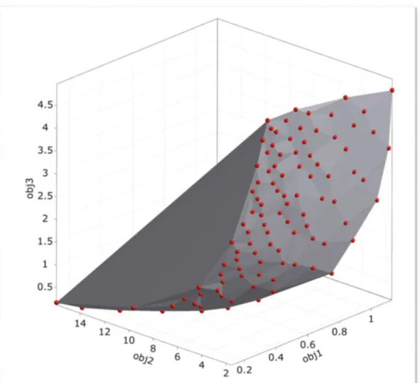
Figure 2.2 illustration of a 3D pareto front for a multi-objective algorithm with three objectives.
2.1.1 Mono-objectivization Techniques
As we will see in the next section, although in literature has been proposed several methods to tackle with the problem of multi-objective optimization, there exists a big gap between the number of research on mono-objective techniques and objective ones. Then, a common approach is to convert the multi-objective problem in a multi-objective one (this is usually called mono-objectivization). Any multi-objective optimization problem may be converted to a single objective optimization problem by aggregating the objectives into a scalar function : → .
One scalarization method, known as weighted sum approach, associates a real weight wi with each objective fi. Accumulating the weighted objective values
yields the combined objective value:
2.2 Metaheuristics
Due to the practical importance of CO problems, many algorithms to tackle them have been developed. These algorithms can be classified as either complete or approximate algorithms. Complete algorithms are guaranteed to find for every finite size instance of a CO problem an optimal solution in bounded time. Complete methods might need exponential computation time in the worst case. This often leads to computation times too high for practical purposes. Thus, the use of approximate methods to solve CO problems has received more and more attention in the last 30 years. In approximate methods we sacrifice the guarantee of finding optimal solutions for the sake of getting good solutions in a significantly reduced amount of time.
Among the basic approximate methods we usually distinguish between constructive methods and local search methods. Constructive algorithms generate solutions from scratch by adding, to an initially empty partial solution components, until a solution is complete. They are typically the fastest approximate methods, yet they often return solutions of inferior quality when compared to local search algorithms. Local search algorithms start from some initial solution and iteratively try to replace the current solution by a better solution.
In computer science and mathematical optimization, a metaheuristic is a higher-level procedure or heuristic designed to find, generate, or select a heuristic (partial search algorithm) that may provide a sufficiently good solution to an optimization problem, especially with incomplete or imperfect information or limited computation capacity. Metaheuristics sample a set of solutions which is too large to be completely sampled. Metaheuristics may make few assumptions about the optimization problem being solved, and so they may be usable for a variety of problems.
The field of metaheuristics for the application to combinatorial optimization problems is a rapidly growing field of research. This is due to the importance of combinatorial optimization problems for the scientific as well as the industrial world. The field of metaheuristics for the application to combinatorial optimization problems is a rapidly growing field of research. This is due to the importance of combinatorial optimization problems for the scientific as well as the industrial world. In the last 20 years, a new kind of approximate algorithm has emerged which basically tries to combine basic heuristic methods in higher level frameworks aimed at efficiently and effectively exploring a search space. These methods are nowadays commonly called metaheuristics. The term metaheuristic, first introduced in 1986 by Glover, derives from the composition of two Greek words. Heuristic derives from the verb heuriskein which means “to find”, while the suffix
meta means “beyond, in an upper level”. Before this term was widely adopted, metaheuristics were often called modern heuristics.
A metaheuristic is formally defined as an iterative generation process which guides a subordinate heuristic by combining intelligently different concepts for exploring and exploiting the search space, learning strategies are used to structure information in order to find efficiently near-optimal solutions. Example of this class of algorithms includes Ant Colony Optimization, Evolutionary Computation including Genetic Algorithms (GA), Iterated Local Search, and Simulated Annealing.
Metaheuristics are typically high-level strategies which guide an underlying, more problem specific heuristic, to increase their performance. The main goal is to avoid the disadvantages of iterative improvement and, in particular, multiple descent by allowing the local search to escape from local optima. This is achieved by either allowing worsening moves or generating new starting solutions for the local search in a more “intelligent” way than just providing random initial solutions.
Summarizing, we outline fundamental properties which characterize metaheuristics:
Metaheuristics are strategies that “guide” the search process.
The goal is to efficiently explore the search space in order to find (near) optimal solutions.
Techniques which constitute metaheuristic algorithms range from simple local search procedures to complex learning processes.
Metaheuristic algorithms are approximate and usually non-deterministic. They may incorporate mechanisms to avoid getting trapped in confined areas of the search space.
The basic concepts of metaheuristics permit an abstract level of description.
Metaheuristics are not problem-specific.
Metaheuristics may make use of domain-specific knowledge in the form of heuristics that are controlled by the upper level strategy.
Today more advanced metaheuristics use search experience (embodied in some form of memory) to guide the search.
In short, we could say that metaheuristics are high level strategies for exploring search spaces by using different methods. Two very important concepts in metaheuristics are intensification and diversification. The term diversification generally refers to the exploration of the search space, whereas the term intensification refers to the exploitation of the accumulated search experience.
In general, two main families can be distinguished in metaheuristics: trajectory-based techniques and population-based methods.
Metaheuristics working on single solutions are called trajectory methods and encompass local search-based metaheuristics. They all share the property of describing a trajectory in the search space during the search process.
Population-based metaheuristics, on the contrary, perform search processes which describe the evolution of a set of points in the search space. In this project, the use of population-based metaheuristics.
As we stated before, Population-based methods deal in every iteration of the algorithm with a set (i.e., a population) of solutions rather than with a single solution. As they deal with a population of solutions, population-based algorithms provide a natural, intrinsic way for the exploration of the search space. Yet, the final performance depends strongly on the way the population is manipulated. The most studied population-based method in combinatorial optimization are Evolutionary Algorithms (EAs) and Behavioral techniques. EAs are based in the principles of the natural evolution, and the population of individuals is modified by recombination and mutation operators. On the contrary, Behavioral techniques, such as Ant Colony Optimization (ACO) or Particle Swarm Optimization (PSO), are based on the emerging behavior of a set of animals. For example, in ACO a colony of artificial ants is used to construct solutions guided by the pheromone trails and heuristic information. In this project, we focus on the popular Evolutionary Algorithms which are described in the next section
2.2.1 Evolutionary Algorithms
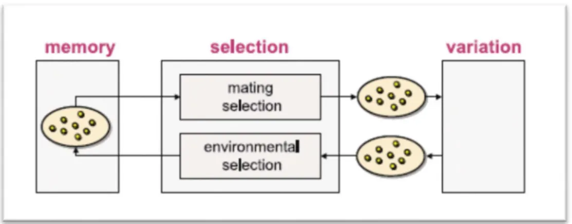
The term evolutionary algorithm (EA) stands for a class of stochastic optimization methods that simulate the process of natural evolution. The origins of EAs can be traced back to the late 1950s, and since the 1970s several evolutionary methodologies have been proposed, mainly genetic algorithms, evolutionary programming, and evolution strategies. All of these approaches operate on a set of candidate solutions. Using strong simplifications, this set is subsequently modified by the two basic principles: selection and variation. While selection imitates the competition for reproduction and resources among living beings, the other principle, variation, imitates the natural capability of creating ”new” living beings by means of recombination and mutation [12]. An evolutionary algorithm is characterized by three features:
1. A set of solution candidates is maintained,
Figure 2.3 Components of a general stochastic search algorithm.
By analogy to natural evolution, the solution candidates are called individuals and the set of solution candidates is called the population. Each individual represents a possible solution, i.e., a decision vector, to the problem at hand; however, an individual is not a decision vector but rather encodes it based on an appropriate representation.
The mating selection process usually consists of two stages: fitness assignment and sampling. In the first stage, the individuals in the current population are evaluated in the objective space and then assigned a scalar value, the fitness, reflecting their quality. Afterwards, a so-called mating pool is created by random sampling from the population according to the fitness values. For instance, a commonly used sampling method is binary tournament selection. Here, two individuals are randomly chosen from the population, and the one with the better fitness value is copied to the mating pool. This procedure is repeated until the mating pool is filled.
Then, the variation operators are applied to the mating pool. With EAs; there are usually two of them, namely the recombination and the mutation.
Although the underlying mechanisms are simple, these algorithms have proven themselves as a general, robust and powerful search mechanism. In particular, they possess several characteristics that are desirable for problems involving i) multiple conflicting objectives, and ii) intractably large and highly complex search spaces.
2.2.2 MOEAs
Generating the Pareto set can be computationally expensive and is often infeasible, because the complexity of the underlying application prevents exact methods from being applicable. For this reason, a number of stochastic search strategies such as evolutionary algorithms, tabu search, simulated annealing, and ant colony optimization have been developed: they usually do not guarantee to
identify optimal trade-offs but try to find a good approximation, i.e., a set of solutions whose objective vectors are (hopefully) not too far away from the optimal objective vectors.
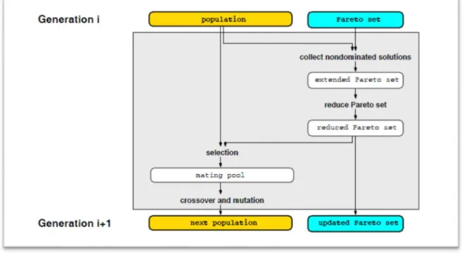
In concrete, Evolutionary algorithms (EA) have proved to be well suited for optimization problems with multiple objectives due to their inherent parallelism they are able to capture a number of solutions concurrently in a single run. Since evolutionary algorithms (EAs) work with a population of solutions, a simple EA can be extended to maintain a diverse set of solutions. With an emphasis for moving toward the true optimal region, an EA can be used to find multiple Pareto-optimal solutions in one single simulation run.
Figure 2.4 Evolutionary search of Optimal Pareto Front
The utilization of EAs to solve MOPs (Multi-Objective Problems) is a current and very promising research line. An entire domain called MOEAs (Multi-Objective Evolutionary Algorihms) is devoted to this research [1].
In MOEA design: guiding the search towards the Pareto set and keeping a diverse set of nondominated solutions. It is considered to be a set of mutually nondominated solutions, or Pareto set approximation for short. Most MOEAs try to maintain diversity within the current Pareto set approximation by incorporating density information into the selection process: an individual’s chance of being selected is decreased the greater the density of individuals in its neighborhood. This issue is closely related to the estimation of probability density functions in statistics, and the methods used in MOEAs can be classified according to the categories for techniques in statistical density estimation.
The MOEA algorithms have certain goals that should be matched; the first goal is mainly related to mating selection, in particular to the problem of assigning scalar fitness values in the presence of multiple optimization criteria. The second goal concerns selection in general because we want to avoid that the population contains mostly identical solutions (with respect to the objective space and the decision space). Finally, a third issue which addresses both of the above goals is
elitism, i.e., the question of how to prevent nondominated solutions from being
lost.
For the first goal we distinguish aggregation-based, criterion-based and Pareto-based fitness assignment strategies. For the second goal most MOEAs try to maintain diversity within the current Pareto set approximation by incorporating
density information into the selection process: an individual’s chance of being
selected is decreased the greater the density of individuals in its neighborhood. For the third goal, elitism addresses the problem of losing good solutions during the optimization process due to random effects. One way to deal with this problem is to combine the old population and the offspring, i.e., the mating pool after variation, and to apply a deterministic selection procedure—instead of replacing the old population by the modified mating pool. Alternatively, a secondary population, the so-called archive, can be maintained to which promising solutions in the population are copied at each generation. Improved algorithm NSGAII (from NSGA) is an elitist procedure which will be described later in section 3.7.
2.3 jMetal Framework
Instead of starting development from scratch, we decided to use the already built-in library called jMetal. It has many algorithms built, ready to use. It is a framework for multi-objective optimization with metaheuristics developed by a research team in the Languages and Computer Science Department of the University of Málaga.
jMetal stands for Metaheuristic Algorithms in Java, and it is an object-oriented Java-based framework for multi-objective optimization with metaheuristic techniques. jMetal provides a rich set of classes which can be used as the building blocks of multi-objective techniques; this way, by taking advantage of code-reusing, the algorithms share the same base components, such as implementations of genetic operators and density estimators, thus facilitating not only the development of new multi-objective techniques but also to carry out different kinds of experiments. The inclusion of a number of classical and state-of-the-art algorithms, many problems usually included in performance studies, and a set of quality indicators allow not only newcomers to study the basic principles of multi-objective optimization with metaheuristics but also their application to solve real-world
problems. The jMetal project is continuously evolving and new versions are released when new features are added.
2.3.1 Design Goals
jMetal´s Developers had on mind this tool should be simple and easy to use, portable (hence the choice of Java), flexible, and extensible. We detail these goals next [9-10]:
Simplicity and easy-to-use. These are the key goals: if they are not fulfilled, few people will use the software. The classes provided by jMetal follows the principle of that each component should only do one thing, and do it well. Thus, the basis classes (SolutionSet, Solution, Variable, etc.) and their operations are intuitive and, as a consequence, easy to understand and use. Furthermore, the framework includes the implementation of many metaheuristics, which can be used as templates for developing new techniques.
Flexibility. This is a generic goal. On the one hand, the software must incorporate a simple mechanism to execute the algorithms under different parameter settings, including algorithm specific parameters as well as those related to the problem to solve. On the other hand, issues such as choosing a real or binary-coded representation and, accordingly, the concrete operators to use, should require minimum modifications in the programs.
Portability. The framework and the algorithms developed with it should be executed in machines with different architectures and/or running distinct operating systems. The use of Java as programming language allows to fulfill this goal; furthermore, the programs do not need to be re-compiled to run in a different environment.
Extensibility. New algorithms, operators, and problems should be easily added to the framework. This goal is achieved by using some mechanisms of Java, such as inheritance and late binding. For example, all the MOPs inherits from the class Problem, so a new problem can be created just by writing the methods specified by that class; once the class defining the new problem is compiled, nothing more has to be done: the late binding mechanism allows to load the code of the MOP only when this is requested by an algorithm. This way, jMetal allows separating the algorithm-specific part from the application-specific part.
2.3.2 Main Features
It includes the implementation of a large number of classic and modern multi-objective optimization algorithms: NSGAII, SPEA2, PAES, PESA-II, OMOPSO, MOCell, AbYSS, MOEA/D, Densea, CellDE, GDE3, FastPGA, IBEA, SMPSO, SMPSOhv, MOCHC, SMS-EMOA, dMOPSO, adaptive and random NSGA-II.
Since real-world problem are used to be very time consuming task, this framework also include some parallel (multithreaded) versions of MOEA/D, NSGA-II and SMPSO (referred as to pMOEAD, pNSGANSGA-II, and pSMPSO, respectively).
The framework also allows to calculate the most popular multi-objective metrics such as Hypervolume, Generational Distance, Spread and Generalized Spread, Error Ratio …
In spite the framework is devoted to multi-objective optimization also some mono-objective algorithm are supported such as generational and state steady Genetic Algorithms, PSO and other classical methods.
Finally, it has also implemented a rich set of multi-objective test problems:
Problem families: Zitzler-Deb-Thiele (ZDT), Deb-Thiele-Laumanns-Zitzler (DTLZ), Walking-Fish-Group (WFG) test problems), CEC2009 (unconstrained problems), and the Li-Zhang benchmark. –
3. Problem Description and Our Approaches
In the previous chapter, we give a brief introduction about optimization, specially focus on multi-objective problems and the current approaches to solve this kind of optimization. Now, in this chapter, we present the problem solved in this project: Test minimization in Software Product Lines. Firstly, we describe the mathematical model of this combinatorial problem, and later, we analyze the techniques used to deal with.
3.1 Test Minimization Problem Introduction
Test minimization techniques aim at identifying and eliminating redundant test cases from test suites in order to reduce the total number of test cases to execute, thereby improving the efficiency of testing. In the context of software product line, we can save effort and cost in the selection and minimization of test cases for testing a specific product by modeling the product line.
However, minimizing the test suite for a product requires addressing two potential issues: 1) the minimized test suite may not cover all test requirements compared with the original suite; 2) the minimized test suite may have less fault revealing capability than the original suite.
We will use different multi-objectives algorithms in order to get a minimized test suite that cover all test requirements and that have same fault revealing capability as the original suite.
For testing a product line, in the current practice of industry, a test suite is typically developed to test the whole product line and the test suite will be modified as new products come into play or the current products need to be improved. However, as the number of products increases, the number of test cases for testing the product line will also increase. Therefore, it becomes practically impossible to execute all the test cases of the product line due to limited available time and resources for each new product. It is therefore essential to seek a solution to minimize test suites for a specific product efficiently before execution to reduce the cost of testing.
3.2 Feature Model and Component Family Model
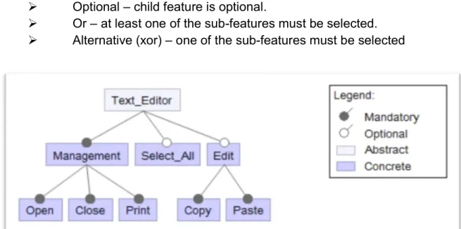
The methodology used to support automated test case selection are Feature Model (FM) which gives you a complete and compact representation of all features of the products of the Software Product Line (SPL) and Component Family Model (CFM) [5].
FM are arranged in a tree-like structure when each successively deeper level in the tree corresponds to a more fine-grained configuration option for the SPL variant. Then parent-child and cross-tree relationships capture the constraints that must be adhered to when selecting a group of features for a variant
FM can be represented as FM = {features, relations, constraints}. It contains four different types of relations among features, namely mandatory, alternative, optional and or]. A mandatory relation between a father feature and a child feature specifies that, if the father feature is included in the current selection, then the child feature must also be included. An alternative relation among a father feature and a set of children features is used when the selection of only one of the children is required, not less, not more. An optional relation is used when the selection is optional. An or relation is used when any number of children features can be selected, but at least one. Sum up:
Mandatory – child feature is required. Optional – child feature is optional.
Or – at least one of the sub-features must be selected. Alternative (xor) – one of the sub-features must be selected
Figure 3.1: Example of a tree representing a Feature Model in Software Product Lines.
CFM can be represented as CFM = {components, parts, source elements, restrictions}. CFM can be used to represent how products are assembled and generated in a Product Line by modelling relations among software architectural elements. It has a hierarchical structure including items such as components and parts. For the purpose of automatic product generation from a valid selected feature model in PL, these items can be organized and used with relevant information about the concrete architecture.
CFM can be represented as CFM = {components, parts, source elements, restrictions}. Components are named entities and organized into a tree-like
structure that can be of any depth. Each component represents one or more functional elements of the products in PL such as functions of software or documentation. Parts are named and typed entities. Each part belongs to a component and contains one or more source elements. A part can be associated with given programming language features, classes or objects, but it can also be associated with other key elements. A source element is an unnamed but typed entity. Source elements are usually used to determine how the source code for the specified element is generated. Restrictions play a key role for linking FM and CFM. A restriction constrains the relationships between an element in CFM and features in FM. They are added into CFM in order to decide whether an element can be part of a product in PL. An element in CFM cannot be associated with a product unless restrictions defined on the element evaluate to true.
In our modelling, CFMs are not used to represent software architecture, but rather to model the hierarchical structure of test cases. This methodology captures the commonalties and variability of a product line using a FM and the domain knowledge of test experts using a CFM.
3.3 Problem Modelling
Summing up and taken into account what said before, what we want is achieving these three objectives [6]:
Minimizing the number of test cases (Test Minimization Percentage, TMP).
Maximizing feature Pairwise Coverage (Feature Pairwise Coverage, FPC).
Maximizing capacity of fault detection (Fault Detection Capability, FDC).
These objectives will be deeply described in the next section. In the literature, we can found some technical proposals based on finding an optimal solution using genetic algorithms that combine these objectives in a balanced way (GAs based on weight vectors). In our case it is proposed to optimize all targets simultaneously using multi-objective techniques. But before of analyzing the techniques, we are going to give a formal definition of the problem.
A product line P that have a set of products P = {P1, P2, P3,…,Pnp} where
Pnp is the number of products of P. P can be represented as a model of
characteristics with a set F = {f1, f2, f3, …, fnf} where fnf is the number of
characteristics or functionalities we wish to test in product line P. To test P, there are a set of test TS = {t1, t2, t3,…, tnt} that comprises a great number of test cases
Search a solution Sk (Skis made up of {tsk1, tsk2, tsk3,…, tntsk}) 1) TMPsk(less
number of test cases); 2) FPCsk(high pair feature coverage) y 3) FDCsk (high fault
detection capability).
3.4 Definition of the Objectives
1. TMP: Measures quantity reduction on the number of test cases and is calculated: 100 * 1 pi sk sk nt nt TMP
where ntsk number of test cases for solution Sk where 1<= ntsk <= ntpi.
ntpi is the number of test cases to test the product Pi, that is one of the products to
test in production line P. The value range of TMP can vary from 0 to 1 and the greater the number is, the greater will be the reduction of needed test cases.
2. FPC: is used to measure how much pairwise coverage can be achieved by a chosen solution. We chose this type of coverage based on our domain knowledge, discussion with test engineers, and history data about faults because a higher percentage of detected faults are mainly due to the interactions between features. FPC is designed to compute the capability of covering feature pairs by a chosen solution, which is computed as below:
% 100 _ _ _ pi sk sk sk FP Num FP Num FP Num FPC
Num_FPsk is the number of feature pairs covered in the test cases for the solution sk, which can be measured as follows:
intskNum FPtci FP
Num_ sk 1 _
where ntsk is the number of test cases for the solution sk, where
1<=ntsk<=ntpi. NUM_FPtci is the number of unduplicated feature pairs covered by
the test case i (tci). The feature pairs covered by tci can be computed as:
NUM_FPtci = Csize2 (Ftci)where size(Ftci) is the number of features tested by that test
case. For instance, if test case tci is used to test three features. Then the feature
pairs covered by test case i 2 3
C = 3*2/2 = 3.Notice, repeated pairs will be removed when computing.
NUM_FPpi is all number of feature pairs for testing the product pi which can
representing the product Pi, including ntpi features. For instance, if Pi is represented
by ten features, all feature pairs covered by the product are 2 10
C = 10* 9/2 = 45. Note that FPC is calculated for a chosen test solution and ranges from 0 to 1 and a higher value of FPC shows higher feature pairwise coverage.
3. FDC measures the fault detection capability of a selected test solution for a product. In out context, fault detection refers to the success rate of a test case in a given time, e.g., a week or a month. In our context, a test case is defined as a success if it can detect faults in a given time and as a fail if it does not detect any fault. The success rate of a test case can be measured as below:
= +
where NumSuctci: is the number of success executions for the given test
case i during the given time; y NumFailtci, is the number of fail executions for the
given test case i during the given time.
3.5 Fitness Function Definition (for Mono-objective Version)
To ease computation of the fitness function, the values for all the three objectives have been normalized by the above-proposed formulas, which range from 0 to 1. We adopted a fitness function based in the normalization of the three objectives, and is defined as follows:
Min Fitness = 1 – (w1 * TMP + w2 * FPC + w3 * FDC)
where w1 + w2 + w3 = 1.
Using this way, multi-objective optimization problem is converted to a single objective problem with a scalar objective function, which is a classical approach and is efficient to be solved using GAs. You can give several different values to the weights depending on the importance given to each objective, to real test those weights can be defined based in systematic methods such as domain analysis, questionnaire. In the original paper [6] the authors propose two variants (based in domain analysis and discussions with Cisco test engineers):
w1 = w2 = w3 = 1/3 and w1 = 0.2, w2 = w3 = 0.4.
3.6 Requirements
The algorithms proposed to solve this problem should fulfill the following requirements:
1. Generated test case set must cover all requirements that the initial test case set.
2. Minimized Generated test case must have same fault detection capability than the original
3. Computing time must be as low as possible since we plan to tackle very large instances.
3.7 Description of Selected Multi-objective Algorithms
In order to solve the previous problem, we have selected three different algorithms. Two of them are well-known MOEA algorithms: NSGAII [7] and SPEA2
[3]. We also use a random multi-objective search to base in our multi-objective comparison.
3.7.1. Non-dominated Sorting and Sharing Genetic Algorithm (NSGAII)
This is an improved version of original NSGA. The original version has been criticized mainly for following issues:
1) Computational complexity (where is the number of objectives and is the population size)
2) Non-elitism approach
3) The need for specifying a sharing parameter.
NSGAII [2] alleviates all the above three difficulties. Specifically, a fast non-dominated sorting approach with computational complexity O(MN2). Also, a
selection operator is presented that creates a mating pool by combining the parent and offspring populations and selecting the best (with respect to fitness and spread) solutions. Simulation results on difficult test problems show that the proposed NSGA-II, in most problems, is able to find much better spread of solutions and better convergence near the true optimal front compared to Pareto-archived evolution strategy and strength-Pareto EA (elitist property). The primary reason for this is their ability to find multiple Pareto-optimal solutions in one single simulation run.
The behavior of NSGAII is as follows. The population is initialized as usual in Genetic Algorithms. Once the population in initialized the population is sorted based on domination into each front. The first front being completely non-dominant set in the current population and the second front being dominated by
the individuals in the first front only and the front goes so on. Each individual in the each front are assigned rank (fitness) values or based on front in which they belong to. Individuals in first front are given a fitness value of 1 and individuals in second are assigned fitness value as 2 and so on.
In addition to fitness value a new parameter called crowding distance is calculated for each individual. The crowding distance is a measure of how close an individual is to its neighbors. Large average crowding distance will result in better diversity in the population.
Parents are selected from the population by using binary tournament selection based on the rank and crowding distance. An individual is selected in the rank is lesser than the other or if crowding distance is greater than the other. The selected population generates offsprings from crossover and mutation operators.
The population with the current population and current offsprings is sorted again based on non-domination and only the best N individuals are selected, where
N is the population size. The selection is based on rank and the on crowding distance on the last front.
3.7.2 Strength Pareto Evolutionary Algorithm (SPEA2)
SPEA2 [3] uses a mixture of established techniques and new techniques in order to find multiple Pareto optimal solutions in parallel.
Stores the Pareto-optimal solutions found so far externally.
Uses the concept of Pareto dominance in order to assign scalar fitness values to individuals.
Performs clustering to reduce the number of nondominated solutions stored without destroying the characteristics of the Pareto-optimal front.
On the other hand, SPEA is unique in four respects:
It combines the above three techniques in a single algorithm.
The fitness of an individual is determined from the solutions stored in the external Pareto set only; whether members of the population dominate each other is irrelevant.
All solutions in the external Pareto set participate in selection.
A new niching method is provided in order to preserve diversity in the population: this method is Pareto-based and does not require any distance parameter.
powerful and up-to-date MOEA. The main differences of SPEA2 in comparison to SPEA are:
An improved fitness assignment scheme, which takes for each individual into account how many individuals it dominates and it is dominated by.
A nearest neighbor density estimation technique, which allows a more precise guidance of the search process.
A new archive truncation methods that guarantees the preservation of boundary solutions.
3.7.3 Random Search (RS)
Basically we use this algorithm as base to compare our EA algorithm to check if they are really smart or they behave as somewhat random. The basic behavior of this method is as follows:
for(int i = 0; i < MAX_SOLUTIONS; i++){ s = randomSolution();
insertInParetoFront(s); }
It generates as many solutions as we want (in our case so many solutions as evaluations do the rest of algorithms), and then it tries to put it in the Pareto front if it is a non-dominated solution.
3.8 Implementation
For solving the problem, we use the jMetal framework which already has implemented the algorithms but it requires to adapt it to the problem at hands. In this section we describe the main classes developed to tackle with the minimization test cases in software product lines.
3.8.1 Instance Class
We define a new java class to create and read a file with the instance of the problem. For the creation: the format of this file is as follows:
The first line contains a single number representing the number of characteristics.
The rest of lines of file are the different test cases. Each line begins with the number of features covered in each test case followed by the number of characteristic and its success rate.
name of the file, each file name will be “instanciaXX.txt” where XX is {18, 29, 46, 59, 77}. The code to build these files is partially shown in the next paragraph:
public static void CrearFichero(int NumCaracteristicas, String s){ …
for (int r = 0; r < COB.length; r++){
COB[r] = (random.nextInt(10-5)+5); //featurs covered by 5-10 TCs
sumaTestCaseFeature = sumaTestCaseFeature + COB[r]; FeaturesInserted[r] = 0;
}
while(sumaTestCaseFeature > 0){ // While uncovered features exist
for (int k = 0; k < FeaturesInserted.length; k++) FeaturesInserted[k] = 0;
// Generate number of test for each test case (a file line)
NumFeatTC = (random.nextInt((5>NumFeatures)?NumFeatures:5)) + 1; pw.print(NumFeatTC +" ");
for(int cont = 1; cont <= NumFeatTC;cont++){
// Generate a number between 1 and number of total Test Case
randomTCTot = (random.nextInt(sumaTestCaseFeature))+1;
// Search which feature is still not covered in this test case
int feat = buscarFeature(COB, randomTCTot, FeaturesInserted); //Feature covered
FeaturesInserted[feat]++;
COB[feat]--; // Less 1 he number of times a feature is covered
if(COB[feat] == 0) NumFeatures--;
sumaTestCaseFeature--; // One less to the total of TC
// Write in file number of feature and success rate pw.print(feat+1+" "+(random.nextInt(successRate)+50) + " "); }
pw.println(); }
}
Example of generated file: 18 2 12 93 6 58 3 10 71 2 62 11 57 3 13 51 15 55 16 63 2 18 76 13 52 5 3 85 8 92 17 92 6 80 4 64 5 16 67 7 71 15 64 17 78 8 71 5 13 87 14 74 17 88 5 53 2 81 2 6 81 7 76 2 8 81 2 89 5 10 87 15 65 11 83 14 61 12 66 1 4 52 5 18 92 1 84 13 92 5 72 16 88 4 13 77 14 59 8 72 1 61
The first line indicates that this software product lines has a FM with 18 different features. The first test case (second line) covers two features: the feature 12 (with a success ratio of 93%) and the feature 6 with 58% of detecting a failure. The interpretation of the rest of the lines is similar.
The method to read generated file will be used in SimpleProblem class, basically we return the content of the file in Vector<Vector<NodoInstance>> structure having as input parameter a String with the name of the file, we use the scanner wrapper to get the content of the file and we insert each pair of integer found in this structure, as we have the number of features covered for each test case at the beginning of the line. The resulting code is:
public Vector<Vector<NodoInstance>> readFile(String filename) { …
while(sc.hasNextInt()) //While is data in the file
{
Vector<NodoInstance> tc = new Vector<NodoInstance>(); // New TC
int nFCovered = sc.nextInt(); // # features covered by this TC
for(int i= 0; i < nFCovered; i++){
NodoInstance n = new NodoInstance(); // Create NodoInstance
n.feature = sc.nextInt(); // Insert number of feature
n.percentage = sc.nextInt(); // Insert success rate
tc.add(n); // Add to the intermediate node
}
data.add(tc); // Add to the returning structure
}
sc.close(); return data; }
3.8.2 Problem Class
This is maybe the most important class since this include the representation of the solution and how the objectives are calculated.
This class uses the Instance one to obtain the data of the current instance and using this information perform the appropriate calculations. This class include several methods (to define the number of objectives, length of the solution and its representation, how an initial solution is generated …) but the most important one is the evaluation of a solution.
The calculations are not simple and they should be performed as efficient as possible since this method is called very frequently. In the next code, we summarize the implementation of that method (all the details and the auxiliary methods are included in the source code files attached to this document):
public void evaluate(BinarySolution solution){
double TestCaseNum, ValidTestCases = 0;
double TMP; //Test Minimization Percentage
double FPC; //Feature Pairwise Coverage
double FDC; //Fault Detection Capability
double FDC_Numerador = 0;
double PairF = 0; //Pair features covered by test suite
Vector<NodoInstance> pairF = new Vector<NodoInstance>();
double arr[] = new double[ncarac];
for (int cont = 0; cont < arr.length; cont++) arr[cont] = 0;
BitSet bitset = solution.getVariableValue(0) ;
for (int i = 0; i < nbits; i++) {
if(bitset.get(i)){
ValidTestCases++;
//Calculate feature pairs covered by test case i
NumPairF(Datos, i, pairF);
arr = calcularFDC(Datos, i, arr); }
}
PairF = pairF.size(); TestCaseNum = Datos.size();
//TMP i equals to --> (1 - (ValidTestCases / NumberOfTestCases if (TestCaseNum != 0)
TMP = (1 - (ValidTestCases / TestCaseNum)); else
TMP = 0;
//NumTC * (NumTc-1) dividido por 2
int TotalF = (ncarac * (ncarac -1)) / 2; //Feature Pairwise Coverage (FPC)
if (TotalF != 0)
FPC = PairF/TotalF; else
FPC = 0;
for (int h = 0; h < arr.length; h++) FDC_Numerador += arr[h];
FDC = FDC_Numerador / ncarac;
//Set the three objectives
solution.setObjective(0, 1-TMP); solution.setObjective(1, 1-FPC); solution.setObjective(2, 1-FDC); }
3.8.3 NSGAII Class
This is the main class, it is used to launch algorithm NSGAII, standard template from jMetal is used with some modifications we have to amend. Basically we have to run NSGA 150 times (30 iterations for each of the 5 files created in the Instance class).See Pseudocode below:
public static void main(String[] args) throws Exception { int arr[] = {18,29,46,59,77};
for (int k = 1; k <= 30; k++){ for (int x:arr){
String nameFile = " instancia"; // Instance name
nameFile = nameFile + x + ".txt"; //compose instance file name
// Call SProblem with the instante filename
SProblem problem = new SProblem(nameFile);
// Other parameters and operators for the algorithm CrossoverOperator crossover = new SinglePointCrossover(0.9); MutationOperator mutation = new
BitFlipMutation(1.0/problem.getBitsPerVariable(0)); SelectionOperator selection = new BinaryTournamentSelection();
// Configure the algorithm
Algorithm al = new NSGAII(problem, // Problem
20, // Max Iterations
100, // Population size
crossover, // Crossover Operator
mutation, // Mutation Operator
selection, // Selection Operator
new SequentialSolutionListEvaluator() // Solution Evaluator
);
// Execute the algorithm
al.run();
// Obtain the results of the execution
List<BinarySolution> l = (List<BinarySolution>)al.getResult();
FileWriter file = null; PrintWriter pw = null;
// Compose name of the output result filename
String Filename = "NSGAII_SP/resultadoNSGAII_"+x+"_"+k+".txt"; file = new FileWriter(Filename);
pw = new PrintWriter(file);
for(int i = 0; i < l.size(); i++){
DefaultBinarySolution s = (DefaultBinarySolution) l.get(i);
pw.println(s.getVariableValueString(0) + "\t" +
s.getObjective(0) + "\t" + s.getObjective(1) +"\t" + s.getObjective(2)); // Write results in output file
} pw.close(); } } } 3.8.4 Other Classes
In the previous subsection, we have describe the main methods of the principal classes developed in this project but other auxiliary classes has been implemented to the make easy the analysis of the results.
Also, SPEA2 and RS classes have been created to run these multi-objective algorithms but the code is very similar to the NSGAII and therefore, their code has not included in this document.
Finally, we have also run two different GA for the mono-objective case. For these experiment we have to create several classes but they are similar to some of the classes previously described (Instance, Problem, or Algorithm ones).
4. Experimental Results
This chapter is divided into two parts: the first one present the experimental design (benchmark, statistical analysis used, parameterization …) while the second part shows the different results obtained. The discussion of the results has been organized also in two analysis: we first compare the different multi-objective among them and then we compare the results of our multi-objective approaches against the existing algorithm (mono-objective GA).
4.1 Experimental Design
In this section, the experimental methodology is described. This includes the benchmark used, what metric are used to compare the algorithm, how are the results analyzed and the parameters of the methods.
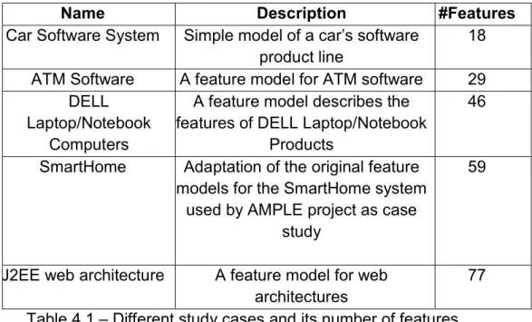
4.1.1 Benchmark
For our tests we have used five products from different SPLOT product lines (http://www.splot-research.org/) [6]. This is a standard repository for this problem. The characteristics of the instances are shown in Table 4.1.
Name Description #Features
Car Software System Simple model of a car’s software
product line 18
ATM Software A feature model for ATM software 29 DELL
Laptop/Notebook Computers
A feature model describes the features of DELL Laptop/Notebook
Products
46 SmartHome Adaptation of the original feature
models for the SmartHome system used by AMPLE project as case
study
59
J2EE web architecture A feature model for web
architectures 77
Table 4.1 – Different study cases and its number of features. All the instances has some characteristics:
Each feature can be tested by 5-10 test cases,
each test case can be used to test 1-5 features and
We generate a file for each instance attending to these requirements using the appropriate method of Instance class (Section 3.8.1).
4.1.2 Quality Indicators
Comparing metaheuristics algorithm is a complex task since these techniques are not deterministic and several independent runs should be performed to each pair algorithm-instance. In multi-objective optimization is even more complex since the result is not a single solution but a set of solutions. Then, we have to clearly define how the algorithms are compared. In this section, we define the metric used to this comparison.
Multi-objective metrics:
Each execution of an algorithm generates a final Pareto Front (PF) which is the set of non-dominated solution found during the search. The metrics usually compare this PF with the optimal Pareto Front (PF*) measuring how similar are these two sets of solutions [11].
The first problem is we don’t know the optimal Pareto front for our problem. We make an approximation to this front, merging the PF found by all the methods (NSGAII, SPEA2, and RS) and obtaining a combining Pareto Front.
Then, several kind of metrics can be defined:
Convergence metrics measure the degree of proximity based on the distance between the solutions in PF* to those in PF. The most used metric for convergence is Generational Distance (GD) which represents the distance between PF and PF*. The smaller is this value, the better is.
Diversity metrics indicate the distribution and spread of solutions in the optimal solution set PF*, we use Generalized Spread (GS) as a metric of this type.
Convergence–Diversity metrics measure the quality of the optimal solution set PF* in terms of convergence and diversity on a single scale. HyperVolume (HV) gives the volume (in the objective space) that is dominated by the optimal solution set PF*. In particular, the closer are the solutions of PF* to the true PFknown,
the larger is the value of HV.
Capacity metrics quantify the number or ratio of non-dominated solutions in PF* that conforms to the predefined requirements. In general, a large number of
non-dominated solutions in PF* is preferred. Error Ratio (ER) is the number of
solutions in PF which are dominated by solutions of PF* [13]. In this case, we are interested in a low value of this metric, which indicates that solutions found are in the optimal Pareto Front.
Mono-objective metrics:
In this case is easier to select a metric to measure the quality of the results. Since each algorithm only generates a single final solution, we’ll use the quality of this solution.
4.1.3 Statistical Analysis
Since we are working with non-deterministic algorithms, each execution can potentially produce different results, and therefor the results of a single execution are not enough to extract any conclusion. Thus we performed 30 independent runs for a meaningful statistical analysis.
Then for each metric described in the previous section (HV, GD …), we have 30 values. In order to make easy the comparison, we need to summarize these 30 values in a single one (or maybe two or three values). We have different alternatives: mean (with standard deviation), median, … To select the most appropriate one, first we check if the underlying distribution of this values follows a Normal distribution or not. We do this using the Shapiro-Wilk test (the confidence level used is 95%, p-value under 0.05). If the data follows the Gaussian distribution, the mean is a good estimator, in otherwise, we will use the median.
In the Appendix, the results of this normality test are shown. There are some cases where the data doesn’t fulfill this test indicating that the data is not following the Normal distribution. Therefore, the values shown in the tables of this chapter will be the median values.
Also, in order to check if the differences between the algorithms are statistically significant or just a matter of chance, we applied the non-parametric test (the data is not Normal) Kruskal-Wallis. Again, the confidence level used is 95%. These results are also shown in the Appendix.
4.1.4 Algorithmic Parameterization
In our experiments, we compared three multi-objective approaches (NSGAII, SPEA2, and RS) and weight-based mono-objective GAs (GA1 with w = (1/3, 1/3, 1/3), and GA2 with w = (0.2, 0.4, 0.4)). For all of GA-based method (all with the exception of RS), we used a standard one-point crossover with a rate of 0.9 and mutation of a variable is done with the standard probability 1/n, where n is the number of variables. Meanwhile, the size of population and maximum number of fitness evaluation are set as 100 and 2000, respectively. Finally, RS was used as the comparison baseline to assess the difficulty of the addressed minimization problems.
4.2 Result Analysis
First, we analyze the different multi-objective technique attending to the different metric described in Subsection 4.1.2 and then we compare these proposed multi-objective approaches with the mono-objective GA proposed by [6].
In the tables, the boldfaced values represent the best results for the instance. The final column indicate in how many instance the algorithm (represented by rows) are the best one in this metric.
4.2.1 Multi-objective Analysis
HV (Hypervolume, larger values are better)
In the next table, the results for the Hypervolume metric are shown. Several conclusion can be obtained from these values. First, the RS is the worst algorithm. This is an expected value since it doesn’t use any information of the problem. The second one is the best algorithm is clearly NSGAII. It outperforms (statistically validated, see Appendix) the results of SPEA2 for all the instances with the exception of the instance with 59 features.
18 29 46 59 77 Total
NSGAII 0.716538 0.625227 0.552107 0.526504 0.533766 4
SPEA2 0.706489 0.606991 0.542786 0.570152 0.509774 1
RS 0.552440 0.435279 0.357473 0.417611 0.368432 0
GD (Generational Distance, lower values are better)
For our next analysis, we use the GD metric. The conclusions are similar to HV one but in this case is even more clear. Again, the RS is the worst algorithm with a large difference (more than one order of magnitude). Also, the NSGAII is the best algorithms, but in this metric it outperforms SPEA2 in all the instances, although the difference for the smallest ones (18, 29, and 46 features) is not statistically significant.
18 29 46 59 77 Total NSGAII 0.006178 0.005524 0.007547 0.005308 0.004430 5
SPEA2 0.006432 0.006018 0.007631 0.005855 0.006018 3
RS 0.026524 0.024704 0.031700 0.022624 0.020620 0
GS (Generalized Spread, larger values are better)
Now, we analyze the spread of the solution in the space solution. On the contrary to the rest of the instances, RS is the algorithm with the best spread. This is a reasonable result since this algorithm makes a uniform exploration of the search space. Then, the solutions found by RS has a very good spread but these solutions are very far from the optimal Pareto Front (as it is shown in previous metrics), and then these solutions are not useful to solve this problem. With respect