Defining and using road network data in an accident database

(1)

Middlesex University Research Repository

An open access repository of

Middlesex University research

http://eprints.mdx.ac.uk

Lupton, Kenneth (1995) Defining and using road network data in an accident database. Masters thesis, Middlesex University.

Accepted Version

Available from Middlesex University’s Research Repository at http://eprints.mdx.ac.uk/13462/

Copyright:

Middlesex University Research Repository makes the University’s research available electronically.

Copyright and moral rights to this thesis/research project are retained by the author and/or other copyright owners. The work is supplied on the understanding that any use for

commercial gain is strictly forbidden. A copy may be downloaded for personal,

non-commercial, research or study without prior permission and without charge. Any use of the thesis/research project for private study or research must be properly acknowledged with reference to the work’s full bibliographic details.

This thesis/research project may not be reproduced in any format or medium, or extensive quotations taken from it, or its content changed in any way, without first obtaining permission in writing from the copyright holder(s).

If you believe that any material held in the repository infringes copyright law, please contact the Repository Team at Middlesex University via the following email address:

[email protected]

(2)

Middlesex University Research Repository:

an open access repository of

Middlesex University research

http://eprints.mdx.ac.uk

Lupton, Kenneth, 1995.

Defining and using road network data in an accident database. Available from Middlesex University’s Research Repository.

Copyright:

Middlesex University Research Repository makes the University’s research available electronically. Copyright and moral rights to this thesis/research project are retained by the author and/or other copyright owners. The work is supplied on the understanding that any use for commercial gain is strictly forbidden. A copy may be downloaded for personal, non-commercial, research or study without prior permission and without charge. Any use of the thesis/research project for private study or research must be properly acknowledged with reference to the work’s full bibliographic details. This thesis/research project may not be reproduced in any format or medium, or extensive quotations taken from it, or its content changed in any way, without first obtaining permission in writing from the copyright holder(s).

If you believe that any material held in the repository infringes copyright law, please contact the Repository Team at Middlesex University via the following email address:

[email protected]

(3)

IN AN ACCIDENT DATABASE

Submitted by

KENNETH LUPTON

for the qualification of

MASTER OF PHILOSOPHY

Middlesex University

September 1995

(4)

Chiefs! Our road is not built to last a thousand years, yet in a sense it is. When a road is once built, it is a strange thing how it collects traffic, how every year as it goes on, more and more people are found to walk thereon, and others are raised up to repair and perpetuate it and keep it alive.

Valima Letters. Address to the Chiefs on the Opening of the Road of Gratitude, October 1894.

(5)

This thesis proposes improvements to the design of road accident databases typically used by local authorities in England. The present design tends to lead to

inconsistencies in the information relating to the road network contained in the database.

A methodology for the redesign of the database is proposed which will lead to greater data integrity and provide

additional and more detailed information. The advantages of the system are demonstrated by producing accident predictive relationships for sharp bends and minor junctions.

The design has been carried out in the context of a relational database system incorporating data from a geographical information system. The advantages of an object-oriented system are also considered and proposed as a direction for further research.

(6)

ACKNOWLEDGEMENTS

The author would like to thank Professor Chris Wright and David Jarrett for their help in preparing this thesis, and also the local authorities who

(7)

S(X) Sk(X) S'k(X) S"k(X) f.1i 'YJi g E(Y) D l(b;y)

'A

spline function polynomial function

first derivative of polynomial function second derivative of polynomial function curvature of polynomial function

B-spline

sum of weighted squared residuals

spline component representing energy due to bending minimising function for smoothing spline

tangent vector

first additional Bezier point second additional Bezier point third additional Bezier point tension parameter

mean of probability distribution systematic part of a statistical model link function

expected value of variable Y

scaled deviance

log of the maximum likelihood mean of a Poisson distribution Pearson's chi-squared statistic

shape parameter of a prior gamma distribution scale parameter of a prior gamma distribution mean of a posterior gamma distribution

(8)

LIST OF FIGURES

1.1 Study network in East Kent 2

2.1 Bobstar sections 9

2.2 Link and node system 10

2.3 Cartographic database 12

4.1 Hypothetical road and accidents 28

4.2 Accidents near a node 28

4.3 The included angle between two lines PJ/h and P3P4 29

4.4 Unwanted inflection at A 34

4.5 B-splines 35

4.6 Four polynomial segments of a cubic B-spline 35

4.7 Comparison of radii for the cubic and B-spline 37

4.8 Comparison of cubic and B-spline 37

4.9 Comparison of cubic, B-spline and smoothing spline, weight = 1000 40

4.10 Cubic spline, B-spline, and smoothing spline 40

4.11 G-spline 42

4.12 A257 at Wingham in Kent 44

5.1 Comparison of models at low radii 53

5.2 Linear Poisson model 53

5.3 Linear Poisson model weighted by traffic flow 55

6.1 Network example 57

6.2 Addition of bypass 61

6.3 Map layers 62

6.4 Conceptual schema for an accident database 63

6.5 Junction layout 65

6.6 Negative binomial distribution of accidents at minor junctions 67 6.7

m

as a predictor of accidents in the after period 69

(9)

3.1 Redundant and duplicated data 17

3.2a Accident location 18

3.2b J unction type 18

3.3 Data errors associated with redundancy 18

4.1 Road alignment and chainage 27

4.2 Output from accloc. prg calculating accident chainage 29

4.3 Estimated radii, means and standard deviations for the A417 for 43 different spline types

4.4 A257 at Wingham 45

4.5 Absolute differences in curvature 46

5.1 Comparison of linear and exponential model 52

5.2 Comparison of models without and with traffic flow 55

6.1 Link location 58

6.2 Link table 58

6.3 Nodes and connected links 59

6.4 Node table 60

6.5 Addition of bypass 61

6.6 Accidents at junctions 67

(10)

The accident databases currently used by local authorities in the UK are prone to error and provide incomplete information for the analysis of road accidents. This is partly due to the fact that the accident data is not related to an adequate definition of the road network. The purpose of this thesis is to compare the accident database systems

currently in use and to develop a suitable road network definition using digital map data. It is also the intention to demonstrate the benefits of this system by developing accident predictive models using data not available from existing systems.

The overall aim of this work is to make a contribution to the efficiency of road

accident database systems and to gain a more detailed understanding of the factors that influence accidents on the road network.

The data for this thesis was obtained during the 'Road Accident Migration' research project. This was an SERC funded project conducted jointly by Liverpool and Middlesex Universities. The purpose of the project was to establish whether the apparent migration of road accidents following an engineering improvement is a real effect or a statistical artefact [1,2,3]. Research work of this type relies heavily upon the data collected by local authorities during their work in road safety. The results of research provide an understanding of the phenomena of road accidents contributing to the common aim of their reduction. Road accidents are fortunately relatively rare events and can arise from a variety of circumstances. Investigations of this type require a large volume of accurate and reliable data in order to explore the

relationships between the number of accidents and both the permanent and transient features of the road network.

During the migration project data was obtained from 13 local authorities. At Middlesex University data was provided by the Bedfordshire, Buckinghamshire,

(14)

Introduction

subsequently used for migration analysis was provided by the Berkshire, Hertfordshire, Leicestershire and Suffolk County Councils. All of these counties did, however.

provide a variety of accident database systems for comparison.

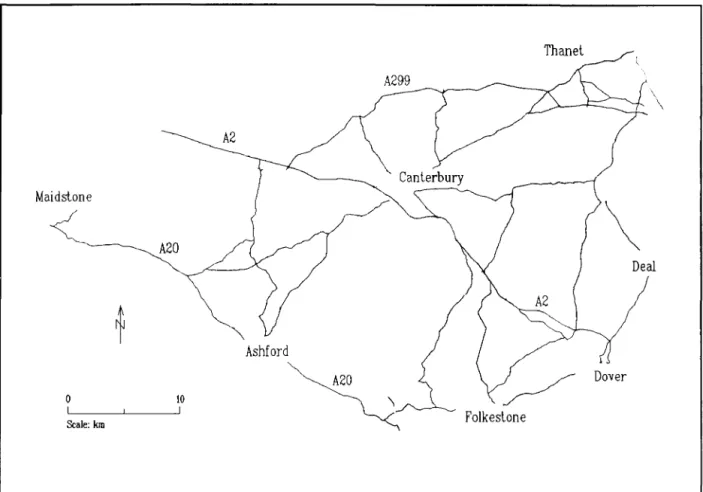
Of the authorities contacted the most detailed road network data was provided by the Kent County Council and it is this data which has mainly been used in this thesis. The network is shown below in figure 1. The roads are a selection of mainly rural major A and B roads in East Kent.

Maidslone ~ o I Scale: km A20 10 I A299 A2 Canlerbury Ashford

~

Figure 1.1 Study network in East Kent

Thanel Folkeslone

\

\ \ Deal

Accident data, traffic flow data and highway improvement data were provided for the roads in Kent over an eight year period from 1984 to 1991. For the purposes of accident analysis parts of the network were not included between 1990 and 1991 where they were significantly affected by the construction of new roads, such as the M20 between Maidstone and Ashford and the dualling of the A299. These improvements caused either a redistribution of traffic or changed the character of the road in a way that were likely to significantly affect the number of accidents.

(15)

Chapter 2 describes various accident databases in use and the methods used for locating accidents on the road. It also describes the parameters currently used for categorising road types recommended by the Department of Transport that are incorporated in their computer program Coba 9. During the thesis some of these parameters will be examined with a view to improving them in the light of more detailed information about the road network from the database.

In chapter 3 fundamental aspects of the relationship between accidents and the road network are considered as the basis for the design of an accident database, assuming the use of a relational database system.

In defining the road network the first consideration is the method of representing the road centre line and this is considered in chapter 4. The possibility of extracting more precise geometry using cubic splines is considered, one advantage being that they can provide an estimate of centre line radius. In chapter 5, an application is demonstrated by examining the relationship between road accidents and curve radius.

After the centre line is defined other aspects of the network definition are considered in chapter 6, such as the method of representing junctions and bypasses. The

potential for defining the road network in more detail using digitised road maps is illustrated by extracting accident data for minor junctions. This data is not easily available using current systems.

In conclusion, chapter 7 discusses the possibilities for using an object-oriented approach to road accident database design.

(16)

2.1 Introduction

Chapter 2

Data Structures

This chapter provides an introduction to database management systems, accident

databases and geographical information systems and reviews the methods for locating accidents that were encountered on the accident migration project. It also describes some of the parameters commonly used to describe the road network in the

Department of Transport cost benefit analysis program COBA9. Some of these

parameters are considered in subsequent chapters with a view to improving them in the light of more detailed road geometry which can be made available from the database.

2.2 Database Management Systems

A database is a collection of non-redundant data which can be shared between different application systems. For example, departments within an organisation may need to view data from the database in different forms depending upon their requirements. Redundant data is data which is repeated unnecessarily in the database and can cause inconsistency in the data. A Database Management Systems (DBMS) is a generalised software interface which allows local views of the data in the database. DBMS have made an important contribution to the availability and coordination of data and their continuing development provides possibilities for the description of the road network in greater detail.

We relate to the road network via the road map which exists at various levels of detail to provide us with the information we require. The availability of maps in digital form facilitates the link between the map and the database which not only makes a large amount of data relating to a road feature immediately available on the computer screen but also enables the spatial relationships of the data to be investigated. These systems are known as Geographical Information Systems and at their core is the cartographic database.

(17)

The accident databases in use by local authorities incorporate the road accident data items recommended by the Department of Transport in the Stats 19 coding form. These items are listed in Appendix A. A variety of methods for locating road accidents were encountered during the research and the databases were generally

designed before the relational database came into being and do not exploit its potential. The purpose of this thesis is to compare the systems in use and to explore their

potential development in order to provide a more detailed and accurate description of the road network. This in turn provides a starting point for a detailed understanding of the relationship between accidents and features of the highway.

The efficient organisation of a local authority is partly dependent upon the ease of access to relevant and accurate data which enables investment decisions to be made most effectively. Increasingly over the past twenty years Local Authorities in the UK have been using computerised data base systems for storing information relating to the road network. DBMS are ideally suited to this purpose as they enable data to be

available to regional offices and other departments from a central computerised system. Central isation avoids the repetition of data where it is required by different offices which can cause inconsistencies when the data is updated. The greater accessibility of data means that a department can make planning decisions that incorporate information that is not within their direct control, for instance, an education department may

require information about road accidents involving school children. In terms of the highway the applications of DBMS are varied:

Road Accidents.

The police provide a detailed description of each road accident that is reported to them. This information is used to establish common factors and trends in accidents and to identify accident blackspots.

Traffic flows.

Automatic traffic counters installed on the highway produce large volumes of accurate data. This data is essential for monitoring trends in traffic growth which in turn enables the implications of alternative regional planning policies

(18)

Data Structures

to be assessed more effectively. The likely effect and cost benefits of new road schemes can also be more accurately predicted.

Maintenance.

A DBMS can be used to store information related to the condition and

maintenance needs of the road network and enable investment decisions to be made with consideration to the needs of the entire network.

The rapid development of database technology means that existing systems can rapidly become out of date and although the new systems may offer considerable advantages the change from one to another may be a difficult and expensive process. An

organisation may be reluctant to undertake a change unless they are quite sure of the benefits. The purpose of this thesis is to consider the methods of organising road accident and the benefits that can be obtained.

2.3 Road Accident Data

The Department of Transport collects road accident statistics from the police

authorities across the country to detect and analyse national trends. The information required is contained in the STATS 19 coding form, see Appendix A. This

information is usually incorporated into the local authority accident database which often contain additional attributes.

An accident database typically consists of three tables:

1. Attendant circumstances. 2. Casualty table.

3. "ehicle table.

Attendant circumstances.

This table contains information relating to the date and location of the accident including the road number and grid coordinates. Data relating to the road environment is included such as road and junction type, speed limit and street

(19)

lighting conditions. It also contains information relating to particular

circumstances surrounding the accident such as the weather conditions and the condition of the road surface.

Casualty table.

This table contains information about the casualties such as the severity of their injuries, their age and sex and whether they were drivers, passengers or

pedestrians. If a casualty is a schoolchild then the name of the school is included.

Vehicle table.

This table includes a description of the vehicles involved such as their type, age and size and their behaviour during the accident. Information pertaining to the driver is included, such as the result of any breath test.

All of this information is usually collected by a police officer present at the scene of the accident.

2.4 Location of Accidents

An important piece of information about an accident which is essential for analysis is its location. The police officer who records the accident locates it by providing a distance to a road feature such as a junction and also by its grid coordinates. The grid coordinates are often not precise, for example, the nearest 100 metres, and local

authorities often implement checking procedures to validate the position. During the accident migration project four systems were encountered for locating accidents:

1. Coordinate system. 2. Chainage system. 3. Bobstar sections. 4. Link and node system.

(20)

Data Structures

Coordinate system.

In this system accidents are located by the road number and Ordnance Survey grid coordinates alone. Manual checking procedures are usually implemented by the local authority to ensure the accuracy of the coordinates. The disadvantage of this system is that no spatial relationship between accidents is available.

Chainage system.

The location of a point on the road is measured usually from Ordnance Survey plans. The start point of the road is usually a junction or local authority boundary. Accidents are easier to locate using this method since the police usually reference them by a distance from a road feature, in addition to their grid coordinates.

Accidents within 20 metres of a junction are usually given a single chainage. In the case of roundabouts an allowance for the distance around junction may be included if the system is also used for road maintenance records.

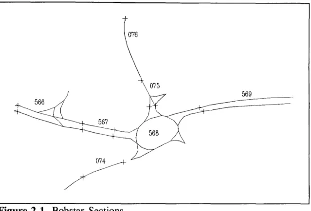
Bobstar sections.

Bobstar is a complete accident database system developed by the Berkshire, Oxfordshire and Buckinghamshire County Councils in the 1970s.

In this system the road is divided into sections that are often approximately 250 metres long in rural areas but this varies from one authority to another. Each section is

intended to contain details of accidents related to the same feature of the road. In some cases the length of a section is approximately inversely proportional to the number of accidents that are likely to occur on that section.

In urban areas the length is usually fixed at 100 metres. Major junctions are also

allocated a section. The start of the section is taken to be 40 metres from the give-way line but again this varies depending upon the junction layout. Sections also start and end at changes in carriageway type, sharp bends, speed limits and local authority boundaries.

(21)

076

075

569

Figure 2.1 Bobstar Sections

Accidents are located by their road number, section number and grid coordinates. The advantage of this system is that it enables accidents relating to a specific road type or feature to be easily identified and is not dependent upon a high degree of locational accuracy. The disadvantage is that in rural areas it incorporates no measure of distance since the length of the sections varies and is generally it is not known precisely.

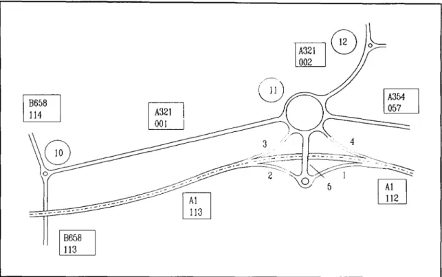
Link and node system

In the link and node system a node is defined as a major junction and has a unique reference number and is located by its grid coordinates. A link is the section of road between two nodes and it has its own chainage system and reference number. Slip roads are referenced to a particular junction and numbered individually.

The link and node system incorporates the advantage of the chainage system in that accidents are easier to locate manually and the chainage provides a spatial relation between them. In the chainage system accidents are allocated a road number and chainage and this means that the accidents for a particular road form a large unit of data which makes search operations inefficient. Dividing the road into I inks reduces

(22)

the size of the data blocks which in turn speeds up search operations.

IB658l

~

IB658l

~

fAll

~

Figure 2.2 Link and node system.

~L

lA32Il

\:J

0

looU

Data Structures

The disadvantage of all four of these systems for locating accidents is that the definition of the road network is not contained within the database and separate

reference must be made to a map. Elements of the network only exist, in effect, after an accident has occurred so it would not be possible to ask the database a question such as "Which major roundabouts had no accidents in 1993?" If one purpose of the database is to identify sites with more than a fixed number of accidents then this may not be a problem; however, if the risk at a site is to be measured by comparison to other similar sites then it is a serious omission. If a lightly trafficked junction

regularly experiences two accidents a year then it may not qualify as a blackspot but if other similar junctions experience none then it is worthy of investigation.

2.5 Geographical Information Systems (GIS) [4,5,6]

A geographical information system is designed to store, manage, display and analyse all types of geographic and spatially related data. A GIS combines a Database

Management System with the ability to represent data in the form of maps and other graphic displays. It has the ability to combine different data sets, for example census information, land use data and highway network data, to form a database which

(23)

enables the modelling of many forms of geographic phenomena.

In a GIS a map is made up of a series of layers each representing a set of geograph ic features; for instance, one layer may display rivers, a second the ground contours and a third land use. The thematic and locational attributes for each layer is held in a table which is part of the cartographic database.

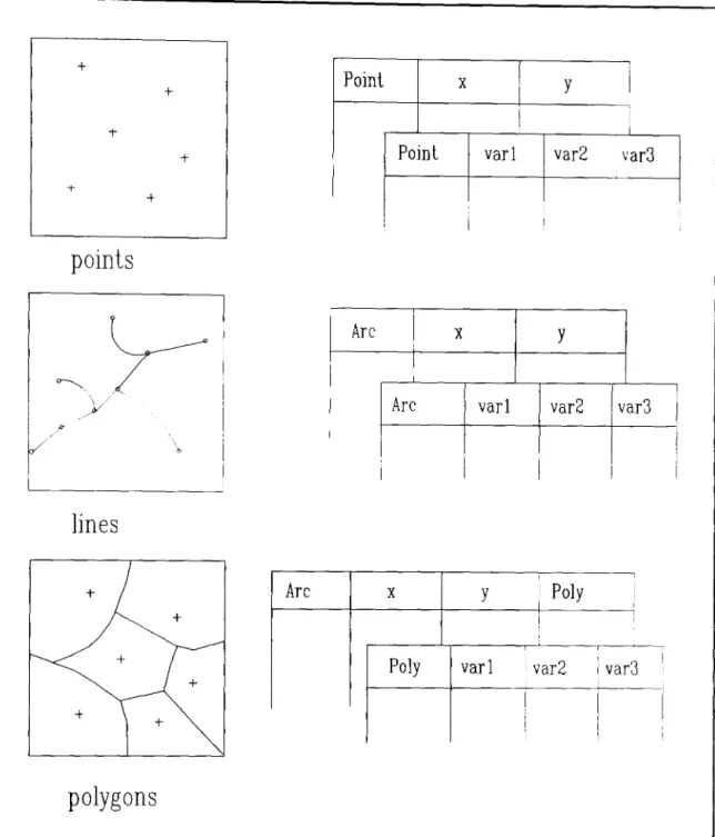
The locational attributes may be stored by three different methods, points, lines and polygons, see figure 2.3. Road accidents would be shown as points, roads and rivers represented by lines and postal districts or land use represented by polygons. A layer may contain a mixture of these types for instance spot levels would be represented by points but contours by polygons. A GIS usually has the facility for calculating the perimeters and areas of polygons.

For the road network a GIS can be used to store information relating to the location of the roads, type of road, maintenance history, traffic flow and accident data. It is

possible to display and analyse entities possessing particular attributes recorded in the database, for example, the number of accidents occurring in the hours of darkness. Since the location of entities is defined, it is possible to identify features within a certain geographical area, for example, it is possible to calculate the distance between a school and the accidents involving pupils of that school.

Advances in technology have made it possible to encode large volumes of digital map data. The location of geographical features can be determined using satellites, known as Global Positioning Systems. Remote sensing and photogrammetry using aeroplanes and satellites are possible sources of data as are existing maps that can be digitised or scanned. These advances combined with improvements in the processing speed and storage capabilities of computers means that a GIS is now a powerful tool for the analysis of traffic related problems.

(24)

Data Structures

+ I

Point x y I

+

-j- i

+ Pojnl varl var2 var3

-j-+ I I _I I i

points

yl

Arc I x y ~ I

Y

Arc varl var2 var3

I

)i' /

r

\

i

b I I I I

lines

-j- Arc x y _!Poly ! + I

+ _Poly _var1 _i_var2

1 var3 ! I + I + _! ! I + I I I ,

polygons

Figure 2.3

Cartographic database.

In practice local authority GIS are developing independently using different digitised maps and software. Ideally all would use a single national system controlled centrally, with each local authority department having access to their relevant data. This would enable accident statistics to be collected at a national level and local authorities to carry out more detailed analysis within the same system. The Ordnance Survey is now

producing a digitised road network, OSCAR, which covers every public road in the country. It is currently available at three levels of detail:

(25)

Network Manager. A simplified representation of the major road for network and route planning.

Route Manager. This represents the adopted road network in a more detailed form but with junctions represented as single nodes.

Asset Manager. Contains detailed large scale road geometry and it includes all public roads and some private roads. It uses a link referencing system with

links identified between each junction and intersection including minor roads. Individual elements of more complex road configurations such as grade separated junctions or roundabouts are also referenced individually.

2.6 Coba 9

The Department of Transport have developed methods for classifying road types for: the calculation of speed flow relationships, travel time costs and the prediction of accidents. These methods are explained in detail in the Department's cost benefit analysis program, Coba 9, reference manual [7].

Coba 9 is a cost benefit analysis program for the economic evaluation of new road schemes. It provides a monetary evaluation of the benefits accrued to the road user over thirty years as savings in:

i) Accidents. ii) Time.

iii) Vehicle operating Costs.

These elements are combined with: i) Capital cost of the schemes. ii) Road maintenance costs.

Coba evaluates the costs of the existing network to provide a basis for comparison for the costs of alternative new schemes.

ACCIDENTS

(26)

Data Structures

Links are classified in terms of road types and nodes, and where appropriate as junction types. Once the traffic flows for these elements are calculated then the

accident rate, expressed in the number of personal injury accidents per million vehicle kilometres, can be estimated from equations developed for Coba. Existing roads are described initially as being rural, speed limit

>

40 mph, or urban, speed limit < 40 mph. The types are:

Rural Urban A B Other Motorway A B Other

Where a link contains a large number of junctions a combined accident rate is given for each category. Junctions are classified according to whether they are rural or urban, their type and their number of arms. The types are:

Major Iminor Traffic signalled Standard Roundabouts Small Roundabouts Mini Roundabouts TIME SAVINGS

Time savings are the major source of cost benefit from a new road. A relationship is required between the traffic flow and vehicle speeds for a given road. Nationally derived relationships for different classes of road are used in Coba. The classes are:

1. Rural single carriageway, nominal width 7. 3m. 2. Rural single carriageway, nominal width 10m.

(27)

3. Rural all purpose dual carriageway. 4. Motorway dual two lanes.

5. Motorway dual three lanes or more. 6. Suburban main road, 40mph speed limit. 7. Urban non-central, 30 mph speed limit. 8. Urban central.

9-12. Special user defined relationships.

The attributes required to determine the speed flow relationships for the category of rural single carriageway roads are as follows:

1. Bendiness; total change of direction per unit distance (deg/km). 2. Hilliness: total rise and fall per unit distance. (m/km).

3. Net Gradient: net rise per unit distance (m/km), one-way links only. 4. Vehicle flow per standard lane (veh/hr).

5. Average carriageway width (m). 6. Verge width.

7. Total number, both sides, of laybys, side roads and accesses, excluding house and field entrances. (no/km).

8. Average sight distance (harmonic mean) (m).

Similar attributes are required for the other road types.

It is apparent that the road network is defined in greater detail for the determination of speed flow relationships than the prediction of accidents. Many of the geometric

variables in Coba are intended to be extracted manually from a plan. The availability of digitised road maps means that they can now be calculated automatically and in some cases there is scope for defining network elements in more detail. In the ensuing chapters some of these possibilities are explored. In the next chapter, however, the fundamental concepts which govern the design of an accident database are considered.

(28)

3.1 Introduction

Chapter 3

Accident Database Design

In this chapter the design principles of the accident database are reconsidered assuming the use of a relational database system. The intention is that this should lead to a more efficient system and one which is less prone to data error. The Department of

Transport require information about road accidents to obtain detailed statistics at a national level. The information required is listed in the Stats 19 coding form and is shown in Appendix A. A local authority database usually incorporates this data plus any local information that they require. It is this data which forms the basis for the database design considerations in this chapter. First it is necessary to describe the principles of relational database design.

3.2 The Relational Database [8]

The relational database system is the most generally used system at the present time. Compared to its predecessors it is more efficient in terms of storage, and is more versatile since it allows data to be extracted and manipulated by the user in many forms depending upon requirements. In a local authority different departments may require information from the same data set. This can be achieved using applications written by the user that are incorporated into the database system. These applications are usually written in the

Structured Query Language,

SQL, a programming language developed specifically for relational databases.

In a relational database the data is divided into subsets called

tables.

A table is made up of columns headed by the name of an

attribute type

and rows, often known as

records.

The intersection of a row and column contains an

attribute value.

The

attribute values that make up a particular row are not interchangeable with those in other rows since the system sets up relationships between them. Columns can be added or removed from the table without compromising its validity, but more

(29)

established between the tables. This relationship can be made by including a

primary

key which is a column, or columns, common to both tables that uniquely defines each row.

3.3 Table Design

The data in a table should be organised so that it is normalised and that it does not contain redundant data. There are three conditions for the normalisation of a table:

1. Each row must be distinct and not duplicated.

2. Attribute values which are not primary keys must be fully dependent upon the primary key.

3. Every non-primary key must be non-transitively dependent upon the primary key.

Redundant data is data which can be eliminated from a table without information being

lost. Duplicated data occurs when an attribute has two or more identical values. These principles are illustrated in Table 3.1 where three separate accidents are recorded at the same junction and the junction number and junction type are

duplicated. The junction number is not redundant since it provides the location of each accident, however the junction type is redundant since it can be found from the

junction number. In this table the junction type is transitively dependent upon the primary key, the accident reference number, and violates rule 3 above. The

redundancy can be eliminated by splitting this table into two normalised tables,

accident location in table 3.2a and junction type in table 3.2b. A relational join can be established between these two tables via the attribute type junction number.

Acc Ref A0001 A0002 A0003 Jnc No J001 J001 J001 RDBT RDBT RDBT

(30)

Acc Ref A0123 A0124 A0125 A0126 A0127 A0128 Acc Ref AOOOI A0002 A0003 Jnc No J001 J001 J001

Table 3.2a. Accident location

Jnc No Jnc_Type

J001 RDBT

Table 3.2b. Junction type

Accident Database Design

Chainage SpJimit St Lights Jnc_Type

1.39 60 Y 1.39 40 +7m Y 1.39 40 +7m T 1.39 60 +7m T 1.39 40 -7m T 1.39 40 -7m T

Table 3.3 Data errors associated with redundancy.

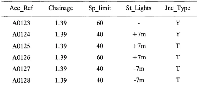
The unnecessary repetition of data is inefficient in terms of the acquisition and input of data and it is also prone to error. Table 3.3 shows six accidents at the same location at different times. Due to the errors in this table it would be difficult to determine the junction type, speed limit or the height of the street lighting at chainage 1.39 with any

degree of confidence.

An alternative explanation for the inconsistency in Table 3.3 is that the junction type, speed limit and street lighting have been changed during the study period. While this

(31)

information is not usually included in an accident database it does illustrate the risks in drawing conclusions after simply inspecting a subset of the data without establishing a structure which governs the type of data to be included in the database.

3.4 Entity relationships.

The relationship between the entity accident and {location,time} is an example of a "one to one" relationship. The relationships between location and accident, and time and accident are both "one to many" relationships since many accidents can occur at the same location at different times and many accidents can occur simultaneously at different locations. Other examples of "one to many" relationships are those between accident and casualties, and accident and vehicle since there may be more than one casualty or vehicle involved in an accident. Each of these is referenced to the accident in which they were involved. One piece of information which is not available is

whether the individual person or vehicle has been involved in more than one accident. This could only be determined by linking the database to census data or vehicle

registration data and this may be considered impracticable.

On the road network, a location can be defined as a combination of road number, and either chainage or grid coordinates, and time by the date, hour and minute of the day. However, this is not necessarily unique as shown in the following situation:

A driver looks across the road at the vehicles travelling in the opposite direction and sees an accident developing, accident A. He is so distracted by this that he drives into the car in front, accident B. Should this be reported as one or two separate accidents?

Since both accidents occur at the same place and time perhaps they should be reported as a single accident but intuitively one might say that they are separate. One solution might be to add the lane number to the definition of location, but this could cause problems in the more common situation where an accident involves vehicles in more than one lane. As an illustration, the following example was taken from an accident database. Two accidents were reported at the same time by two different police

(32)

Accident Database Design

officers on a dual carriageway, one on the northbound carriageway, the other on the southbound carriageway and the verbal descriptions of the accidents are as follows:

1. AI-N. Car towing trailer, vehicle 1, travelling north, struck vehicle 2 also travelling north and crossed the central reservation and struck vehicle 3

travelling south.

2. AI-S. Car travelling south, vehicle 1, was struck by car towing trailer travelling north, vehicle 2, which had crossed the central reservation after colliding with vehicle 3 also travelling north.

In this database the subdivision of the road into two separate carriageway has contributed to the double counting of the same accident.

Returning to the original problem, there is another apparent anomaly if one considers the vehicles involved. Vehicles are included in the database that contribute to the accident and so the vehicles of accident A have contributed to accident B but not vice versa. Including vehicles A in accident B would break the rule that the same vehicle cannot be involved in more than one accident which would lead to the double counting of vehicles. The solution to this problem is offered in the attribute type

carriageway

hazard,

see Appendix A, which can take on the value

previous accident

and is

applicable to accident B.

Another situation is one where a vehicle collides with a stationary vehicle that has been involved in a previous accident. Whether this is reported as one or two accidents usually depends upon the time difference involved. If the second collision occurred seconds after the first collision then it would be reported as one, but if the difference was, say, thirty minutes it would be reported as two. If a circumstance occurs on the road which causes an accident there is an associated probability that a certain number of vehicles will be involved, and also a probability that they will become involved after a certain time interval. To preserve the concept of statistical independence therefore it should be thought of as one accident. However this would lead to a loss of

(33)

information, possibly relating to the effectiveness of precautions taken at the scene of an accident to warn oncoming drivers. Again the attribute value

previous accident

is appropriate, but perhaps these accidents should not be included in any statistical analysis which assumes independence.

An additional requirement of the database can therefore be made that any accident which occurs at a different time or place and may be considered separate to any other accident should be recorded as a unique event.

3.5 Elimination of Redundancy

Recently, Austin [9] has suggested a validation procedure by comparing the recorded locational variables with the same variables defined separately in a GIS. The variables identified were: road class, road number, district, speed limit, pedestrian crossings, junction control, junction detail, carriageway type and markings.

In the attendant circumstances table the non-redundant data is that which is relevant to the accident at the time that it occurred; the redundant data is that which is descriptive of permanent features of the road network unless it describes the location of the

accident. The redundant data is listed as follows:

1.

link number

2. speed limit

3.

road type

4.

junction detail

5.

junction method of control

6. lighting conditions

Within these attribute types however, there are categories that are not permanent features or which may not be defined as part of the network:

Junction detail.

This includes private entrances. It is assumed that the roads defined in the network are those within the jurisdiction of the local authority.

(34)

Accident Database Design

Junction method of control.

This includes control of the junction by an

authorised person who could be included as a separate column.

Lighting conditions.

While the type of lighting is a permanent feature provision must be made to show whether the lighting was on or off at the time of the accident, again this could be recorded separately.

One attribute type that is not included in this list is that of

pedestrian crossing

and this requires more detailed consideration, see attendant circumstances in Appendix A. The categories of crossings are very detailed and it is not appropriate to define all of them in separate tables, for example, it would be impracticable to define every central refuge on the network. However, there is a source of redundancy since there is repetition in the type

pedestrian location

in the casualty table. The reason for this is that a pedestrian may be a contributory factor in an accident without necessarily becoming a casualty. This redundancy can be eliminated by defining the type and location of crossing in a separate table and eliminating central refuge from the attendant circumstances. It has already been mentioned that the presence of an authorised person can be defined separately.

Some authorities include the attribute type

overtaking manoeuvre

which describes the number of vehicles travelling in each direction and the number overtaking. This presumably applies to moving vehicles only. This provides another source of redundancy compared with the attribute type

manoeuvre

in the vehicle table which gives a detailed description in three main categories; overtaking or colliding with stationary vehicles, other moving vehicles or vehicles manoeuvering at junctions. If

overtaking manoeuvre

is intended to apply to vehicles overtaking at speed only then in practice this information is often inaccurate since it tends to be recorded for any overtaking manoeuvre.

Some attribute types in the attendant circumstances table that can be determined from other tables are

severity, number of casualties

and

number of vehicles.

Many SQL implementations incorporate a function that will calculate the day of the week from a

(35)

specified date.

3.6 Enterprise Rules

In order to develop a conceptual model of the database and to eliminate redundant data, it is useful to determine the

enterprise rules

that establish the relationships between different data types, for example that:

1. A casualty is associated with one accident. 2. An accident may involve several casualties.

3. At least one vehicle is associated with one accident. 4. An accident may involve several vehicles.

5. There is one {location, time} associated with each accident. 6. There is one road type associated with each {location, time}.

7. There is one junction type, where applicable, associated with each {location, time}.

8. There is one junction control method associated with each junction. 9. There is one speed limit associated with each {location, time}.

10. There is one type of street lighting associated with each {location,time}.

The database now could be modified to contain the following information in separate tables: Accident detail. 1. Attendant circumstances 2. Casualty 3. Vehicle Network detail 4. Road type 5. Speed limit 6.

J

unction type

(36)

Accident Database Design

7. Street lighting. 8. Pedestrian crossing.

This structure has three main advantages over the current databases which are:

1. The tables are normalised.

2. The network data can be stored in a GIS.

3. Additional network attributes may be added without requiring modifications to the attendant circumstances table.

The development of the network tables will be discussed further in chapter 6.

3.7 Conclusion

The design of the Stats 19 accident database, currently in use by local authorities, was conceived before the advent of the relational database. It contains redundant data which can lead to data errors. The number of errors and the volume of data to be recorded can be minimised by redesigning the database into normalised tables. It has been necessary to develop rules and definitions that govern the data to provide a framework for the database. A major source of redundancy in the present system is that the road network is not defined in separate tables.

The first consideration in defining the road network is the method of representing the road centre line. This problem is considered using data from digitised road maps in chapter 4.

(37)

4.1 Introduction

Highway Geo",etry

There are a number of circumstances where the highway engineer needs to know the geometry of an existing road. When designing the tie-in for a new road the engineer needs to know the precise location of the existing centre line and also its radius to provide a smooth transition. Knowing the centre line radius would also enable the relationship between radius and accidents to be investigated and also the deterioration of skid resistance with radius.

The traditional method of finding the radius of an existing road is to overlay templates of known radii, such as railway curves, on a large scale plan until a satisfactory match

is obtained. Where more precise information is required it is obtained from a site survey.

In the case of a recently constructed road this information may be available from the construction records, but for the majority of roads this does not apply. Many roads have been in existence for centuries and their present alignments are the result of a succession of improvements. Whilst a new road may be designed as a series of straight lines and circular arcs or cubic splines, the alignment of an existing road may be more complex.

In this chapter methods are considered for obtaining geometric information about the road alignment from the data stored within a GIS.

4.2 Centre line data

A digitised road alignment provides new source of information about the geometry of a road. It was decided to explore the possibility of using this data to represent the road more fully. The computation of road geometry was carried out using data supplied by the Kent County Council. The data comprised road alignments that included centre

(38)

Highway Geometry

line and junction detail extracted from their GIS. The data were supplied on disk in the standard drawing interchange format,

dxf.

A

dxf

file is an ASCII file which list the entities and their locations that make up a drawing. These files were viewed and

edited using Autocad since it is a powerful graphics package readily available in the University and is able to import and export

dxf

files.

It was found that the supplied centre lines were made up of a series of short arcs that were not always connected and also were not necessarily in order. Before any centre lines could be defined the arcs had to be sorted into road and chainage order. This was achieved by redrawing the centre lines as single entities using Autocad. First extraneous information such as junction detail and slip roads was removed to leave only the arcs that made up the centre line. The details of these arcs were then stored in a

dxf

file created by Autocad.

A program was written which extracted the coordinates of the end points of the arcs that made up the centre lines from the

dxf

file. The program also produced an

Autocad script file which contained commands for Autocad to replot the coordinates as points. Once the points were plotted a series of connecting lines, or polylines, were then drawn through the points to produce a single centre line for each road. The

coordinates of each centre line, that were now in order, were then extracted once again from a

dxf

file and stored in the relational database system, Foxpr02.

4.3 Road length

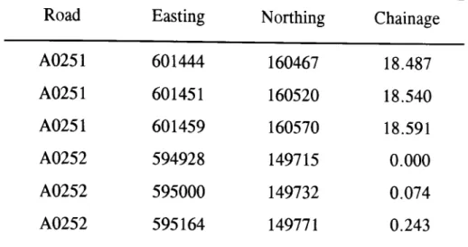
A fundamental description of a road is its length. In order to define a chainage system an SQL program was written which calculated the cumulative distance along the road. This program CHAIN.PRG is listed in Appendix C. Part of the resulting output is shown below in Table 4.1.

(39)

Road Easting Northing Chainage A0251 601444 160467 18.487 A0251 601451 160520 18.540 A0251 601459 160570 18.591 A0252 594928 149715 0.000 A0252 595000 149732 0.074 A0252 595164 149771 0.243

Table 4.1. Road alignment and chainage.

4.4 Accident Location

The accidents on these roads were referenced to this chainage system. Accidents are located by their grid coordinates, that generally are close to but may not lie on the road centre line and so it was necessary to write a program which located the perpendicular offset from the accident to the centre line in order to calculate the

chainage. This is calculated by vector geometry, and the method is shown in detail in Appendix B and summarised here.

First the distance between the start of a centre line arc and an accident is calculated and also the angle between this line and the linle This enables the calculation of the intersection point between the perpendicular offset from the accident and the arc.

Initially a hypothetical road with accidents was used to develop the program, see figure 4.1.

In

figure 4.1 it is clear which section of road each accident is related to, however some accidents have perpendicular offsets to more than one link, for example a8 has offsets to three links.

In

order to select the correct link a zone, nominally 20 metres wide, was defined either side of the centre line and only accidents that fell within this zone were allocated a chainage on that link. This also provides a check on the

accident location since any accident erroneously placed outside of this boundary might well have a lateral error also. Accidents not within the boundary appear in the output with a chainage of zero. They were then relocated to their correct position according to the accident record.

(40)

Highway Geometry

There is an additional problem in the vicinity of nodes, see figure 4.2. Accident al is within the boundary and has an offset to both links, whereas a2 does not have an offset to either link. The solution was to locate accidents within a 20 metre radius of a node and to give those the chainage of the node. The program ACCLOC.PRG is

listed in Appendix C and a sample of the output in table 4.2 .

pl .... p2 " "

"

__

~-

+

a3 " "

--

"

+

a1

----

---- .... _{" / "}" --- " " " a4 -- -- >'"" "

+ ""

/

"

... / / / / / \ / / --... '. / ----...-...'. , / / a8

+\-.,.(-

a6/+/

---

/ p5

----

:.r-. _ / / ... -...-..-... ...

---__ +

a7 centre line zone offset

----

---Figure 4.1 Hypothetical road and accidents.

---\

--- 20m _~1

Figure 4.2 Accidents near a node.

/ / p4//

"

/ / / /

"

Y / p3 / " / / / / / /

+/

a5 / / /

(41)

ACCID ROAD EASTING NORTHING CHAINAGE A3045 A0257 620731 157528 5.70 A3046 A0257 620742 157523 5.71 A3047 A0257 620756 157516 5.72 A3048 A0257 620822 157477 5.81 A3049 A0257 620633 157470 5.82 A3040 A0257 620903 157422 5.90

Table 4.2 Output from Accloc. prg calculating accident chainage.

4.5 The representation of digitised horizontal alignments

In order to calculate speed-flow relationships COBA incorporates the variable

bendiness

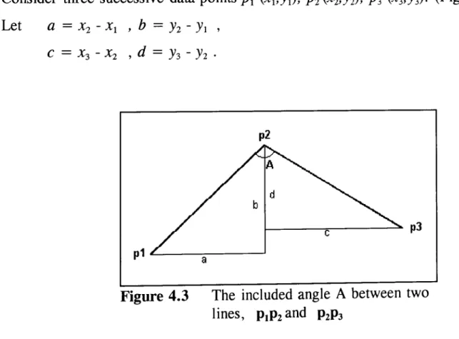
in order to represent the variability of the horizontal alignment. Bendiness is defined as the total change in direction per unit distance (deg/k). This variable can be readily calculated knowing the deflection angle between digitised centre line arcs. The deflection is estimated as follows:

Consider three successive data points _{PI (XI,YI)' pz (xz,Yz), P3 (X3'Y3)'} (Figure 4.3). Let a = _{Xz -} Xl , b = Yz - YI ,

C

=

X3 - Xz ,d

=

Y3 - Yz .

p2

I---..---~ p3 p1 L-.. _ _ : : - -_ _ - '

Figure 4.3 The included angle A between two lines, PIP2 and P2P3

(42)

the distance l2 from P2 to P3 =

v (e

+tf)

the direction cosines for Pl to _{P2 alll, bill} the direction cosines for P2 to _{P3 cll2, dll2}

The angle A between the two lines is given by the expression

Highway Geometry

This calculation has been implemented in the Foxpr02 program ANGMES.PRG, see Appendix C.

The availability of digitised road alignments allow a more detailed representation of the alignment. In the Bobstar system sharp bends are allocated a section, however the radius is not included. Highway engineers have used cubic splines for the design of horizontal alignments for a number of years and an investigation was carried out to assess the feasibility of fitting splines to a digitised alignment. When designing a road the designer fixes the curve at a few pinch points and allows the spline to develop a natural shape between. For a digitised alignment, however, the data points are far more numerous and close together and so the spline has more constraints. The investigation was carried out using data made available by the Kent County Council and the Oxfordshire County Council whose alignments were digitised from the 1/ 1250 and 1/2500 Ordnance Survey.

4.6 Cubic Splines [10]. Theoretical Considerations.

It is possible to construct a single polynomial which passes through any given set of data points, however, functions of this type can produce undesirable oscillations. A more reliable method is to piece together a series of lower order polynomials, or splines, that pass through successive points. The resulting curve is therefore made up of a series of shorter overlapping curves or splines. There are two requirements for this method, firstly that the curve should fit the data points with a smooth alignment and secondly that a sufficient number of conditions should be specified to enable the

(43)

If the curve is to have a smooth appearance then at the point where two splines meet, known as a

knot,

they should have the same radius of curvature. This implies that the curvature should be continuous. The second derivative of the polynomial should therefore be at least a linear function. The minimum order of polynomial that satisfies this condition is the cubic.

Consider the

n+

1 points (x",yJ where Xo

<Xl < ...

<xn The function S(x) is called a cubic spline if there exist

n

cubic polynomials Six) such that:

1.

S(x)

=

Sk(X)

=

Yk

+

Skl(X-XJ

+

Sk2(X-XJ2

+

Sk3(x-XJ3

2. When x

=

_Xkthen Six)

=

Yk .

The spline passes through each data point. 3. Six) = Sk+ I (x).

The spline forms a continuous function.

4. S'k(X)

=

S'k+l(X).

If the first derivatives are equal then the slope is continuous.

5. S"ix)

=

S"k+l(X).

If the second derivatives are equal then the curvature is continuous.

Two additional conditions, the

endpoint constraints,

enable the calculation of the spline. If the endpoint constraints are that the curvature is zero then this is the condition for a natural cubic spline. Since most road alignments start and end at a junction where the curvature of the centre line less important than the junction layout this is the condition that has been used.

The curvature S"(x) when plotted against x forms a set of linear splines, where

S\(x) exists if _xk

<

=

X

<

_=Xk+l and k

=

0,1, ... n-l. Any point on this system of

(44)

Highway

Geometry Integrating this equation and incorporating the above conditions yields the following cubic expression,

where _{m_{k }} _{represents the curvature which can be calculated from the expression}

hk-1mk_1

+

2(hk_1

+

hJmk

+

h~k+l = Uk

Uk

=

6(dk - dk-l) for k

=

1 to n-l and d

=

(Yk+l-Y \ Ihk _Vi, and h _k ₌ x _k+l-Xk

where

for k = 1 to n-l.

These equations together with the endpoint constraints yield the following system of linear equations

2(h_o_+hl) _hI ₀ ₀ _m 1 hI _{2(hl +hJ h}_z 0 _m_z 0 hn -z 0 _{0 h}_{n -}_z 2(h_n__z+h n-l) mn -l

or, more compactly as

A.m

=

U

U₁

U_z

=

U_{n -}₁

Matrix A is a tridiagonal matrix, that is it has non-zero elements on the three central diagonals only. This set of equations can be solved by Gaussian elimination. In this method the equations are modified so that all values below the leading diagonal

computed to be zero. If all of the elements in the first and second rows are divided by the first non-zero elements in each row and then first row is subtracted from the

second then the first element in the second row is then zero. This process is repeated for all of the rows. Since the last row will only contain one value this equation can be solved directly which enables the solution of the preceding rows. In this way the whole system of equations can be solved.

(45)

4.7 Parametric Representation

[11].

Cubic splines can be calculated provided Xo

<Xl < ...

<Xn , that is there is a unique ordinate for each value of

x.

Road alignments do not usually satisfy this condition since they may be orientated in any direction. Initially a program was written which rotated the road centre line so that it was parallel to the x-axis but this did not always satisfy the condition along the entire road length. It would have been necessary in some instances to split the alignment into shorter sections that would then require piecing together after calculating the splines.

This condition is too restrictive for road alignments and for general data of this type it is more usual to parameterise the spline by curve length. Since initially the curve length is unknown the cumulative straight line distance ch between the data points is often taken to be a sufficient approximation. The curve is then calculated by solving the matrix equation A.m=u for ( ch,x) and then for (ch,y).

Radius of Curvature.

The radius at any point on the curve can be calculated from the expression,

A program CUBSCR. CPP was written to calculate the cubic spline that interpolates a given set of data points and outputs the coordinates of the spline at a specified chainage interval. CUBRAD.CPP calculates the radius of the spline at the same chainage

points. These programs were written in Turbo C+ + since it is a portable language and the algorithms could be incorporated into other applications.

Initially a program was written to extract the digitised centre line coordinates from a

dxf

file and produce a standard text file that could be read by CUBSCR.CPP. The output from CUBSCR.CPP is in the form of an Autocad script file which is a text file containing commands that enable the curve to be plotted in Autocad. CUBSCR.CPP is listed in Appendix C .

(46)

+

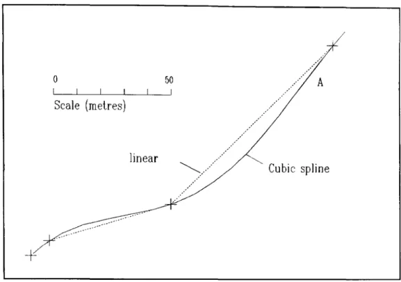
o I Scale (metres) linear 50 _A ... «</«</<//«/« ; / / Cubic spline / . ' /

Figure 4.4 Unwanted inflection at A

Highway Geometry

Cubic splines were fitted to a number of roads using these programs and the resulting curves plotted in Autocad. One disadvantage of the cubic spline is its tendency to insert unwanted points of inflection where none are suggested by the data as shown in Figure 4.4. These points of inflection can be removed by the use of a

shape

preserving

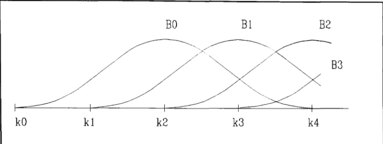
spline, that is, the curve conforms to the shape suggested by the data points. Programs were written to produce such a spline using the properties of the B-spline.

4.8 B-SPLINES [11,12].

The minimum number of intervals required to support a cubic spline is four. The cubic spline which exists only for these five abscissas is known as a basis or B-spline. A curve may be constructed which is a linear combination of such cubic splines. At any point the ordinate on the curve will be equal to the sum of the ordinates of