Quantifying credit portfolio losses under multi-factor models

MODELS

Authors:

Gemma Colldeforns-Papiol Centre de Recerca Matem`atica Campus de Bellaterra, Edifici C 08193 Bellaterra (Barcelona) Spain

and

Departament de Matem`atiques Universitat Aut`onoma de Barcelona 08193 Bellaterra (Barcelona)

Spain

e-mail: [email protected]

Luis Ortiz-Gracia

Universitat de Barcelona School of Economics Faculty of Economics and Business

University of Barcelona John M. Keynes 1-11 08034 Barcelona Spain e-mail: [email protected] Cornelis W. Oosterlee

CWI – Centrum Wiskunde & Informatica NL-1090 GB Amsterdam

The Netherlands and

Delft University of Technology

Delft Institute of Applied Mathematics 2628 CD Delft

The Netherlands

Quantifying credit portfolio losses under multi-factor models

Abstract. In this work, we investigate the challenging problem of estimating credit risk measures

of portfolios with exposure concentration under the multi-factor Gaussian and multi-factor t-copula models. It is well-known that Monte Carlo (MC) methods are highly demanding from the compu-tational point of view in the aforementioned situations. We present efficient and robust numerical techniques based on the Haar wavelets theory for recovering the cumulative distribution function (CDF) of the loss variable from its characteristic function. To the best of our knowledge, this is the first time that multi-factor t-copula models are considered outside the MC framework. The analysis of the approximation error and the results obtained in the numerical experiments section show a reliable and useful machinery for credit risk capital measurement purposes in line with Pillar II of the Basel Accords.

Keywords. Credit risk, Value-at-Risk, Expected Shortfall, Multi-factor models, Gaussian copula, t-copula, Fourier transform inversion, Haar wavelets.

AMS subject classifications. 91G60, 62P05, 60E10, 65T60

1. Introduction

Financial institutions need to evaluate and manage the risk arising from its business activities. Credit risk is the risk of losses from the obligor’s failure to honour the contractual agreements. It is usually the main source of risk in a commercial bank. Banks are subject to regulatory capital

requirements under Basel Accords and they are forced to keep aside a cushion to absorb potential losses in the future. The capital needed in order to remain solvent at a certain confidence level is calledeconomic capital. The basic regulatory risk measure in credit risk is Value-at-Risk (VaR) and it is a quantile of the loss distribution computed with a one-year time horizon at a high confidence level α ∈ (0,1) where the regulatory level for credit risk is α = 0.999. Although it is still the regulatory measure, the VaR value has mainly two drawbacks that may impede a robust credit risk measurement. One of these two disadvantages is that VaR is not sub-additive and contradicts the idea of diversification. The second is that VaR gives no indication about the severity of losses beyond the computed quantile. This is the reason why the Expected Shortfall (ES) might be used in place of the VaR value for internal risk capital assessment (i.e., for economic capital calculation). The Vasicek model forms the basis of the Basel II approach. It is a Gaussian one-factor model where default events are driven by a latent common factor that is assumed to follow a Gaussian distribution, also called the Asymptotic Single Risk Factor (ASRF) model. Under this model, loss only occurs when an obligor defaults in a fixed time horizon. If we assume certain homogeneity conditions, this one factor model leads to a simple analytical asymptotic approximation for the loss distribution and VaR value. This approximation works well for a large number of small exposures but can underestimate risks in the presence of exposure concentrations (see [14]). Concentration risks in credit portfolios arise from an unequal distribution of loans to single borrowers (exposure

or name concentration) or different industry or regional sectors (sector orcountry concentration). While regulatory capital is estimated by means of the ASRF model under Pillar I, economic capital takes into account concentration risks and is calculated under Pillar II. Monte Carlo simulation either with one-factor or multi-factor models (to account for sector concentration or for modelling complicated correlation structures) is a standard method for measuring the risk of a credit portfolio. However, this method is time-consuming when the size of the portfolio increases. Computations can become unworkable in many situations, taking also into account that financial companies have to re-balance their credit portfolios frequently. On top of that, when using MC methods the variance is always an issue when estimating the risk measures at high confidence levels. For the aforementioned reasons, numerical methods are appealing in this field.

Different techniques can be found in the literature for estimating the risk with multi-factor Gaussian copula models, like MC methods in [8], Hermite approximations in [17], where the main application is for large loan or mortgage portfolios (3000 loans), a hierarchical factor model in [6] where closed-form solutions are derived under the assumption that the number of sectors in the portfolio is large, and an extension of the granularity adjustment technique to a new dimension is developed in [18]. However, as pointed out in [11], some works suggested that default events driven by t-distributed random variables provide better empirical fit to the observed data. This is the so-called t-copula model, where default events are expressed as the ratio of a normal and a scaled chi-square random variable. The bivariate version of this last type of models is tackled with simulation in [3, 19] and a complicated multi-factor version in [11].

In the present work, we develop numerical techniques to contribute to the efficient measurement of VaR and ES values for small or big portfolios in the presence of exposure concentration under high-dimensional models. It is worth remarking that small and/or concentrated portfolios are particularly challenging cases, since asymptotic methods usually work out well for large and diversified portfolios. We model the dependence among obligors by means of multi-factor Gaussian copula and multi-factor t-copula models. To the best of our knowledge, this is the first time that multi-factor t-copula models are considered outside the MC framework. We estimate the risk measures in a procedure composed of two main parts. The first part is the numerical computation of the characteristic function associated to the portfolio loss variable. We tackle this part with different techniques depending on the underlying model. For the (bivariate) t-copula model we perform a double integration with Gauss-Hermite and generalized Gauss-Laguerre quadrature, while the multi-factor Gaussian model

is treated with the quadratic transform approximation (QTA) method put forward in [10], where the authors calculate the price of a collateralized debt obligation. We derive the characteristic function for the most challenging model, this is, the multi-factor t-copula, by conditioning on the chi-square random variable of the model and applying the QTA method at each discretization point of the resulting one-dimensional integral. This last model is by far the most involved in terms of computing effort. Once the characteristic function for the loss variable has been obtained, then the second part of the procedure consists of a Fourier inverson to recover its CDF. For this purpose, we use a method based on Haar wavelets developed in [12] for the one-factor Gaussian copula model. Moreover, we have improved the efficiency of this method by computing the coefficients of the expansion by means of an FFT algorithm and we have shown that this method outperforms the well-known numerical Laplace transform inversion method [1, 2] used in risk management in [9, 10] in terms of efficiency and robustness. The numerical experiments carried out in this work show the high accuracy and speed of the method. Another point of importance is the robustness of the wavelet approach. We show how the scale of approximation (this is, the number of terms used to approximate the CDF) is related to the absolute error of the method. All these features make the proposed methodology an efficient and reliable machinery to be used in practice.

The outline of this paper is as follows. We start with the formulation of the credit portfolio losses problem in Section 1.1 and we give a brief overview on Gaussian and t-copula models for dependence among obligors in Section 1.2. We derive the characteristic functions for all the models in Section 2. The methodology for the efficient evaluation of characteristic functions is explained in Section 3. In Section 4 we study in detail two inversion methods. Section 5 is devoted to the numerical examples and Section 6 concludes.

1.1. Credit portfolio losses. To represent the uncertainty about future events, we specify a probability space (Ω,F,_P) with sample space Ω, σ-algebra F, probability measure _P and with filtration (Ft)t≥0 satisfying the usual conditions. We fix a time horizon T > 0, where T usually

equals one year.

Consider a credit portfolio consisting ofN obligors. Any obligorncan be characterized by three parameters: the exposure at default En, the loss given default which without loss of generality we assume to be 100% and theprobability of default Pn, assuming that each of them can be estimated from empirical default data. The exposure at default of an obligor denotes the portion of the exposure of the obligor that is lost in case of default. The portfolio loss Lis defined as,

(1) L=

N

X

n=1

Ln,

with Ln being the individual credit loss given by Ln = En ·1Dn, where 1Dn is the event that

obligor n defaults during the risk measurement horizon. We build upon the work in [12] where the one-factor Gaussian copula model was considered as the model framework and we tackle the more involved problem concerning multi-factor models. The one-factor model belongs to the class of structural models and it is a one period default model, i.e., loss only occurs when an obligor defaults in a fixed time horizon. Based on Merton’s firm-value model, to describe the obligor’s default and its correlation structure, we assign to each obligor a random variable called value. The firm-value (or, more precisely, the asset firm-value log-return) Wn of obligor n at time T is represented by a common, standard normally distributed factor Y component (the state of the world or business cycle, usually called systematic factor) and an idiosyncratic noise component Zn,

(2) Wn=

√ ρnY +

p

1−ρnZn,

where Y and Zn, ∀n ≤ N are i.i.d. standard normally distributed and ρ1,· · ·, ρN ∈ (0,1) are

correlation parameters calibrated to market data. In case that ρn=ρ for all n, the parameter ρ is called the common asset correlation. Using the factor structure (2), obligors become independent conditional on Y.

In the Merton’s model, obligor n defaults when its firm-value falls below the threshold level cn, defined by cn := Φ−1(Pn), where Φ−1(x) denotes the inverse of the standard normal CDF. We

can therefore define Dn := {Wn < cn} and the probability of default of obligorn conditional to a realizationY =y is given by,

pn(y) :=P(Dn|Y =y) = Φ _c n− √ ρny √ 1−ρn .

Consequently, the conditional probability of default depends on the systematic factor, reflecting the fact that the business cycle affects the possibility of an obligor’s default.

In Section 2, we move a step forward by considering, on the one hand, multi-factor models to account for sector concentration and, on the other hand, by selecting different copula models like the Gaussian and the t-copula, where the last one is capable of introducing tail dependence in credit portfolios. For the t-copula model we assume that latent random variablesW1,· · ·, WN are

generated by, (3) Wn= r ν V( √ ρnY +p1−ρnZn),

where Z1,· · ·, ZN, Y ∼ N(0,1), V ∼ χ2(ν) and Z1,· · ·, ZN, Y and V are mutually independent.

Again, ρ1,· · ·, ρN ∈ (0,1) are correlation parameters calibrated to market data. Systematic risk factor Y may be interpreted as an underlying risk driver or economic factor, with each realization describing a scenario of the economy. Random variables Z1,· · ·, ZN represent idiosyncratic, or obligor specific, risk. Scaling the model in (2) by the factor pν/V transforms standard Gaussian random variables intot-distributed random variables with ν degrees of freedom.

As a result, we compute the risk measures by means of both, the multi-factor Gaussian copula model as well as the multi-factort-copula model. Copulas are simply the joint distribution functions of random vectors with standard uniform marginal distributions. Their value in statistics is that they provide a way of understanding how marginal distributions of single risks are coupled together to form joint distributions of groups of risks, that is, they provide a way of understanding the idea of statistical dependence. For sake of completeness, we give in Section 1.2 a review of the dependence structure given by the Gaussian andt-copula models. For further details on dependence and copulas see [13, 19].

1.2. Gaussian and t-copula models. We start this section by focusing our attention to the case in which default dependence is modelled as a multivariate Gaussian process. With the same notation as in Section 1.1, the unconditional probability of default Pn of obligor nbecomes,

P(Dn) =P Wn<Φ−1(Pn), and the joint default probability is given by,

P(1D1 = 1, . . . ,1DN = 1) =P W1 <Φ −1_(P

1), . . . , WN <Φ−1(PN)

.

Let (u1, . . . , uN) = (P1, . . . , PN) be a vector in [0,1]N, and choose a dependence structure described

by correlation matrix Γ. Then, the unique Gaussian copula CΓ associated with (W1, . . . , WN) is, CΓ(u1, . . . , uN) = ΦΓ Φ−1(u1), . . . ,Φ−1(uN)

=P W1 <Φ−1(u1), . . . , WN <Φ−1(uN)

, for any (u1, . . . , uN)∈[0,1]N, where ΦΓ is the multivariate standard Gaussian distribution function

with correlation matrix Γ.

In the same way we can extract a copula from the multivariate normal distribution, we can extract an implicit copula from any other distribution with continuous marginal distribution functions. For example, the (N-dimensional) t-copula takes the form,

Cν,Γ(u1, . . . , uN) = Φν,Γ Φν−1(u1), . . . ,Φ−ν1(uN)

=P W1<Φ−ν1(u1), . . . , WN <Φ−ν1(uN)

, for any (u1, . . . , uN)∈[0,1]N, where Φν,Γis the multivariatetdistribution function with correlation

matrix Γ, and Φ−_ν1 denotes the inverse of the distribution function of a standard univariate t distribution with ν degrees of freedom.

2. Multi-factor firm-value models and their characteristic functions

As mentioned in Section 1, one of the two steps involved in the estimation of risk measures is the efficient computation of the characteristic function associated to the loss random variable L in (1). We consider in Section 2.1 the multi-factor Gaussian copula model, which is the extension from one factor to several factors of model (2) treated in [12, 14]. We consider the t-copula and multi-factor t-copula models in Section 2.2 and Section 2.3, respectively. We tackle these two last models separately for methodological reasons that will be explained later on.

2.1. Multi-factor Gaussian copula. Multi-factor models aim at modelling complicated corre-lation structures. The d-factor Gaussian copula model assumes that the correlation among Wn is introduced by a d×1 vector Y = [Y1, Y2, . . . , Yd]T of independent standard normal random variables, representing the systematic risk factors,

(4) Wn=aTnY +bnZn, n= 1,· · · , N.

Note that we represent vectors by bold symbols throughout the paper. Here,an= [an1, an2, . . . , and]T is a d×1 vector of real constants satisfying aT_nan < 1, which represents the vector of factor

loading coefficients of the common factors, and Zn are N(0,1) random variables representing the idiosyncratic risks, independent of each other and independent of Y. The constant bn, being the factor loading of the idiosyncratic risk factor, is chosen so that Wn has unit variance, i.e., bn=

q

1−(a2_n1+a2_n2+· · ·+a2_nd), which ensures thatWn areN(0,1).

The incentive for considering the multi-factor version of the Gaussian copula model becomes clear when one rewrites it in matrix form,

(5)      W1 W2 .. . WN      =      a11 a21 .. . aN1      Y1+      a12 a22 .. . aN2      Y2+· · ·+      a1d a2d .. . aN d      Yd+      b1Z1 b2Z2 .. . bNZN      .

While eachZnrepresents the idiosyncratic factor affecting only obligorn, eachYj, j= 1, . . . , d, may affect all (or a certain group of) obligors. Although the factors Yj are sometimes given economic interpretations (as industry or regional risk factors, for example), the key role of the factors Yj is that they allow us to model a complicated correlation structure in a non-homogeneous portfolio. More detailed information is available in [10].

Here, the probability of default of obligor n conditional on the realization y ∈Rd of systematic risk factor Y is defined as,

(6) pn(y) :=P(Wn<Φ−1(Pn)|Y =y) = Φ Φ−1_(P n)−aTny bn . Given a realization of the systematic risk factor Y, defaults are independent. Then,

(7) Ee−iωL Y = N Y n=1 Ee−iωEn1{Wn<cn} Y = N Y n=1 1 +pn(y) e−iωEn_−1,

wherecn= Φ−1(Pn) and Φ−1(·) denotes, as usual, the inverse of the standard normal CDF. By the law of iterated expectations, the characteristic function1 ψLof L is therefore given by,

(8) ψL(ω) =Ee−iωL=EEe−iωL Y =E "_N Y n=1 ϑg_n(ω,y) # = Z Rd fY(y) N Y n=1 ϑg_n(ω,y)dy,

where ϑgn(ω,y) := 1 +pn(y)(e−iωEn_{−1) and f}

Y is the d-dimensional standard Gaussian density.

2.2. t-copula with ν degrees of freedom and t-distributed margins. As pointed out in [19], while Gaussian copulas do not exhibit tail dependence, this is, the defaults do not occur simultaneously, t-copula models admit tail dependence, with fewer degrees of freedom producing stronger dependence. We assume that latent random variables W1,· · · , WN are generated by the model specified in (3).

The probability of default of obligorn conditional onY =y and V =v is then given by, pn(y, v) :=P Wn<Φν−1(Pn)|Y =y, V =v =P r ν V √ ρnY +p1−ρnZn <Φ−_ν1(Pn)|Y =y, V =v =P Zn< p v/νΦ−_ν1(Pn)− √ ρny √ 1−ρn ! = Φ p v/νΦ−_ν1(Pn)− √ ρny √ 1−ρn ! .

As pointed out in [20] and because of the conditional independence, the characteristic function of the loss Lnow reads,

ψL(ω) =E e−iωL =E E e−iωL Y, V =E " _N Y n=1 E e−iωEn1{Wn<cn} _{Y, V} # =E "_N Y n=1 ϑn(ω, y, v) # = Z R×[0,+∞) fY(y)fV(v) N Y n=1 ϑn(ω, y, v)dydv, (9)

where the threshold level is defined by cn= Φ−ν1(Pn) and,

(10) ϑn(ω, y, v) := 1 +pn(y, v)(e−iωEn−1), fY is the standard normal probability density function (PDF) of Y,

(11) fY(y) = √1

2πe

−y2_/2

, and fV is the chi-square PDF withν degrees of freedom, i.e.,

(12) fV(v) = 1

2ν/2_Γ(ν/2)v

ν

2−1e−v/2.

Note that we have replaced the joint density of Y and V in (9) by the product of the marginal densities because they are independent random variables.

2.3. Multi-factor t-copula model. In this section, we consider a multi-factor model with depen-dence among obligors driven by a t-copula. We assume that latent random variables W1,· · · , WN

are generated by,

(13) Wn= r ν V a T nY +bnZn ,

whereY, Zn,anandbnare defined and follow the same hypothesis as in Section 2.1, withV ∼χ2(ν) as in Section 2.2. Here the probability of default of obligor n conditional on Y =y and V =v is given by, (14) pn(y, v) = Φ p v/νΦ−_ν1(Pn)−aTny bn ! , the conditional expectation reads,

E e−iωL Y, V = N Y n=1 1 +pn(y, v) e−iωEn , and thus, (15) ψL(ω) = Z Rd_×[0,+∞) fY(y)fV(v) N Y n=1 ϑn(ω,y, v)dydv,

where ϑn(ω,y, v) := 1 +pn(y, v) e−iωEn−1

, fY is the d-dimensional standard Gaussian density

and fV is the chi-square PDF withν degrees of freedom.

3. Efficient computation of characteristic functions

The evaluation of the characteristic function (9) in Section 2.2 in a certain point w, which is a particular case of (15) for d = 1, involves the computation of a double integral that we solve efficiently in Section 3.2.1 by means of numerical quadrature. However, looking at the expressions of the characteristic functions (8) and (15), corresponding to the multi-factor Gaussian and t-copula models, we realize that a direct attempt of solving thed- and (d+ 1)-dimensional integrals, respectively, at fixed points w is not affordable with numerical integration. For these challenging tasks, we rely on the QTA put forward in [10] for computing the Laplace transform of the portfolio loss within the multi-factor Gaussian copula model. We first introduce the QTA method in Section 3.1 and use it to calculate the characteristic function (8). We show in Section 3.3 how we can benefit from the QTA approach for the challenging case of the multi-factor t-copula of Section 2.3 by conditioning on the V factor.

3.1. Multi-factor Gaussian copula. We start this section by enunciating the proposition which forms the basis of the QTA method.

Proposition 1 (Proposition 1 of [10]). Let Z be a d×1 vector of independent standard normal variables. For any scalar c∈C, vector g∈Cd, and matrix H ∈Cd×d for which <(H) is negative-semidefinite,

(16) Ehec+gTZ+ZTHZi= p 1

det(I−2H)e

c+gT_(I−2H)−1_g/2

,

where <(z) denotes the real part of z.

First of all, let us define the mappings7→gn(s) for n= 1,· · ·, N as,

(17) gn(w, s) := 1 + e−iωEn_−1Φ Φ −1_{(Pn) +s}p aT nan bn ! , s∈R. Thus, one can rewrite the conditional expectation (7) as follows,

(18) E e−iωL Y = N Y n=1 gn(w, Sn) = e PN n=1lngn(w,Sn)_{, whereS} n:=− aT_nY p aT nan . If we approximate lngn(w, Sn) by a quadratic function ofSn,

(19) lngn(w, Sn)≈αn(w) +βn(w)Sn+γn(w)Sn2,

where the scalars αn(w), βn(w) and γn(w) are complex-valued, then one can use (18), (19) and Proposition 1 to obtain a closed-form approximation for ψL in (8),

(20) ψL(ω) =E h ePNn=1lngn(w,Sn)i_≈Eh_ePNn=1(αn(w)+βn(w)Sn+γn(w)S2n) i =Ehec(w)+gT(w)Y+YTH(w)Yi.

The last equality follows from the fact thatSn’s are linear inY. The scalarc, vector g, and matrix H are given explicitly by,

(21) c(w) = N X n=1 αn(w), g(w) =− N X n=1 βn(w)an p aT nan , and H(w) = N X n=1 γn(w) anaTn aT nan .

In order to obtain the coefficients (αn(w), βn(w), γn(w)) we make use of the weighted least-squares method. We will go into the details in the numerical examples section.

3.2. t-copula withν degrees of freedom andt-distributed margins. If we replaceϑn, fY and fV in expression (9) by their corresponding expressions (10), (11) and (12), we obtain the iterated integral, (22) ψL(ω) = 1 √ 2π2ν2Γ ν 2 Z +∞ 0 vν2−1e− v 2 Z R e−12y 2 YN n=1 e−iωEn_−1p n(y, v) + 1 dy ! dv. We propose in Section 3.2.1 a numerical integration method to evaluateψL(ω) in (22) at a fixed point w. We show in Section 3.2.2 how the one-dimensional version of the QTA method can be applied by conditioning on the V factor. We will compare the efficiency of both methods in the numerical experiments section and show that in this case, numerical integration is superior to the QTA method.

3.2.1. Numerical integration. We solve the inner integral in (22) by Gauss-Hermite quadrature and the outer integral by generalized Gauss-Laguerre quadrature. For sake of completeness we briefly review both quadrature methods. In numerical analysis, Gauss-Hermite quadrature is a particular type of Gaussian quadrature for approximating the value of integrals of the form,

Z R e−x2f(x)dx. In this case, (23) Z R e−x2f(x)dx≈ nh X i=1 wif(xi),

wherenh is the number of sample points used. Thexi, i= 1,2,· · · , nh, are the roots of the Hermite polynomial of degreenh,Hnh(x), and the associated weights wi are given by wi=

2nh−1_n h!

√

π nh2[H_nh−1(xi)]2.

Generalized Gauss-Laguerre quadrature is an extension of the Gauss-Laguerre quadrature method for approximating the value of integrals over R+ with integrands of the form xαe−xf(x) for some real number α >−1. Precisely,

(24)

Z +∞ 0

xαe−xf(x)dx.

This allows us to efficiently evaluate such integrals for polynomial or smooth f(x) even when α is not an integer. In this case,

Z +∞ 0 xαe−xf(x)dx≈ nl X i=1 wif(xi),

wherexi is thei-th root of Laguerre polynomial of degreenl,Lnl(x), and the weightwi is given by

wi = _(n xi

l+1)2[Lnl+1(xi)]2. Finally, if we perform the change of variables y =

√

2x in (22), and apply the quadrature rules (23) to the inner integral and (24) to the outer integral, then,

ψL(ω) = 1 √ π2ν2Γ ν 2 Z +∞ 0 vν2−1e− v 2 Z R e−x2 N Y n=1 ϑn(ω,√2x, v)dx ! dv ≈ √ 1 π2ν2Γ ν 2 nl X i=1 wl_i   nh X j=1 w_jhϑ(w, x˜ h_j, vl_i)  , (25) where ˜ϑ(w, x, v) = QN n=1ϑn(w, √ 2x, v), and wh

j, xhj are the weights and sample points in Gauss-Hermite quadrature andw_il, v_ilare the weights and sample points in the generalized Gauss-Laguerre quadrature. We observe that the computational complexity of evaluating the numerical formula (25) for a fixed valuew isO(nl·nh).

3.2.2. One-dimensional QTA method. Let us start by enunciating the one-dimensional version of formula (16) in Proposition 1.

Corollary 1. Let Z be a standard normal random variable. For any scalars c, g, h∈C, for which

<(h)≤0,

Ehec+gZ+hZ2i= _p 1 (1−2h)e

c+₂₍₁g₋2_2h)

.

Proof. Follows immediately from Proposition 1 by consideringd= 1.

The key idea in this section is conditioning on the factor V in (3) and applying Corollary 1 for each fixed value v of V. Looking at expression (9),

(26) ψL(ω) = Z R×[0,+∞) fY(y)fV(v) N Y n=1 ϑn(ω, y, v)dydv,

we observe that we can write,

(27) ψL(ω) = Z +∞ 0 fV(v)E h Ehe−iwL(v)|Yiidv= Z +∞ 0 fV(v)E h ePNn=1lngn(w,Y,v)i_dv,

where L(v) emphasizes the fact thatV takes a fixed valuev and,

gn(w, y, v) := 1 + e−iωEn_−1Φ p_v νΦ −1 ν (Pn)− √ ρny √ 1−ρn ! , for (y, v)∈R×[0,+∞). We can compute E h ePNn=1lngn(w,Y,v) i

using a similar approximation as in Section 3.1,

(28) lngn(w, Y, v)≈αn(w, v) +βn(w, v)Y +γn(w, v)Y2, and applying Corollary 1,

EhePNn=1lngn(w,Y,v)i_≈Eh_ec(w,v)+g(w,v)Y+h(w,v)Y2i = _p 1 1−2h(w, v)e c(w,v)+₁₋g2(_2hw,v_(w,v)₎ , (29) for<(h(w, v))≤0 and, (30) c(w, v) = N X n=1 αn(w, v), g(w, v) = N X n=1 βn(w, v), and h(w, v) = N X n=1 γn(w, v).

Hence, from (27) and (29) we end up with,

(31) ψL(ω)≈ Z +∞ 0 fV(v) ec(w,v)+ g2(w,v) 2(1−2h(w,v)) p 1−2h(w, v) dv = 1 2ν2Γ ν 2 Z +∞ 0 vν2−1e− v 2e c(w,v)+₂₍₁g₋2(_2hw,v_(w,v) ₎₎ p 1−2h(w, v) dv. We solve the integral in (31) by means of generalized Gauss-Laguerre quadrature. It is worth remarking the dependence on v for the coefficients c(w, v), g(w, v) andh(w, v). As a consequence, this method involves N quadratic approximations of the type in (28) for each discretization point considered in the quadrature rule.

3.3. Multi-factor t-copula model. In a similar manner as in Section 3.1 and Section 3.2.2, we define, gn(w, x, v) := 1 + e−iωEn−1 Φ pv νΦ −1 ν (Pn) +x p aT nan bn ! , for (x, v)∈R×[0,+∞).

With this notation we can rewrite, N Y n=1 ϑn(ω,Y, v) = N Y n=1 gn(w, Xn, v)) =ePNn=1lngn(w,Xn,v)_{, forXn=−} a T nY p aT nan .

For eachn, we approximate lngn(w, Xn, v) by a quadratic function in Xn, lngn(w, Xn, v)≈αn(w, v) +βn(w, v)Xn+γn(w, v)Xn2, and then, N X n=1 lngn(w, Xn, v)≈ N X n=1 αn(w, v) + N X n=1 βn(w, v)Xn+ N X n=1 γn(w, v)Xn2 =c(w, v) +gT(w, v)Y +YTH(w, v)Y, where, c(w, v) = N X n=1 αn(w, v), g(w, v) =− N X n=1 βn(w, v)an p aT nan , and H(w, v) = N X n=1 γn(w, v)ana T n aT nan .

If we follow a similar procedure as in Section 3.2.2 and we apply Proposition 1, then the characteristic function in (15) can be approximated as,

ΨL(ω)≈ Z +∞ 0 fV(v)E h ec(w,v)+gT(w,v)Y+YTH(w,v)Yidv = 1 2ν2Γ ν 2 Z +∞ 0 vν2−1e− v 2 1 p det(I−2H(w, v))e c(w,v)+gT(w,v)(I−2H(w,v))−1g(w,v)/2_dv, (32)

where c(w, v) ∈ C, g(w, v) ∈ Cd is a vector, H(w, v) ∈ Cd×d is a matrix, I is the d-dimensional identity matrix and fV(v) is the PDF of a chi-square distribution with ν degrees of freedom. We want to underline that in order to apply Proposition 1 we need<(H) to be negative-semidefinite. In the numerical examples section, we will explain how to proceed when this condition is not satisfied. We compute the integral in expression (32) by generalized Gauss-Laguerre quadrature.

4. Inversion methods

Central to the methodology presented in this work is an efficient method to carry out the inversion of characteristic functions. We have seen in Section 3 that characteristic functions of the loss Lare known (numerically) for multi-factor Gaussian and t-copula models. We devote the present section to the numerical method selected to perform the inversion step. Let fL and FL be the PDF and CDF of L, respectively. Without loss of generality we assume that the sum of the exposures En is one, this is, PN

n=1En= 1. Then,

(33) FL(x) =

Fc(x), if 0≤x≤1, 0, ifx >1,

for a certainFcdefined in [0,1]. Recall thatψLis the Fourier transform of the densityfLand then,

(34) ψL(ω) = Z R e−iωlfL(l)dl= Z R e−iωlF_L0(l)dl,

whereF_L0 is the derivative of distribution functionFLin the context of generalized functions. If we integrate by parts,

(35) ψL(ω) =e−iω+iω

Z 1 0

e−iωlFc(l)dl,

and then the Fourier transform of Fc is given by,

(36) Fˆc(w) = ψL(ω)−e

−iω

iω .

We aim at recoveringFcfrom its Fourier transform ˆFc. For this purpose, we use the metod initially developed in [12] for Laplace transform inversion and further extended in [15] for Fourier transform inversion, where numerical errors are studied in detail as well. It is based on Haar wavelets (for a deep insight in wavelets we refer the reader to [4]) and called WA. The method is presented in Section 4.1 where this time we have computed the coefficients with the FFT to speed up the overall

inversion process. We briefly recall in Section 4.2 how to calculate the VaR (as in [12]) and the ES (as in [14]). In Section 4.3 we show the popular method [1, 2] for numerical Laplace transform inversion (NLTI), since it is used in our main reference paper [10] and it was also used in [9] for credit portfolio losses. We make a comparison against the WA method in terms of accuracy and speed.

The choice of Haar basis seems natural since the CDF of L is a piecewise constant function. In [16] the authors show how the WA method compares to the state-of-the-art COS method [5] for Fourier inversion in the framework of credit portfolio losses. It is shown that COS produces oscillations in the tail leading to non-reliable risk measures.

4.1. Haar wavelet approach. The WA method is based on a wavelet expansion of the CDF of L using Haar wavelets as scaling functions. For the sake of completeness, we give a brief overview of the theory of approximation by wavelets.

Consider the spaceL2(R) ={f :R_−∞+∞|f(x)|2dx <∞}. For simplicity we can view this set as the set of functions f(x) which get small in magnitude rapidly asx goes to plus and minus infinity. A general structure for wavelets inL2(R) is called a Multi-resolution Analysis (MRA). We start with a family of closed nested subspaces,

...⊂V−2 ⊂V−1 ⊂V0⊂V1 ⊂V2⊂..., inL2(R) where, \ j∈Z Vj ={0}, [ j∈Z Vj =L2(R), and, f(x)∈Vj ⇐⇒f(2x)∈Vj+1.

If these conditions are met, then there exists a functionφ∈V0such that{φj,k}k∈Zis an orthonormal basis of Vj, where,

φj,k(x) = 2j/2φ(2jx−k).

The function φ, called the father function, generates an orthonormal basis for each Vj subspace. For any f ∈L2(R) a projection map of L2(R) ontoVm,

Pm :L2(R)→Vm, is defined by means of,

(37) P_mf(x) =X

k∈Z

cm,kφm,k(x),

where cm,k =

R+∞

−∞ f(x)φm,k(x)dx are the scaling coefficients. The right-hand side of (37) gives a sum in terms of the scaling functionsφm,k. Considering higherm values (i.e., when more terms are used), the truncated series representation of the function f improves.

To develop our work we consider Haar wavelets (see [4]). Using these wavelets, Vj is the set of L2_{(R) functions which are constant on each interval of the form [}k

2j,k₂+1j ) for all integers k. In this

case the father function is given by,

φ(x) =

1, if 0≤x <1, 0, otherwise,

As opposed to Fourier series, a key fact about using wavelets is that wavelets can be moved (choosing the k value), stretched or compressed (choosing thej value) to accurately represent the local properties of a function. Moreover,φj,k is non-zero only inside the interval [₂kj,

k+1

2j ). In what

follows we make use of this fact to compute VaR without the need of knowing the whole distribution of the loss function.

In our case, we approximate Fc in (33) by a finite combination of Haar scaling functions at a fixed scale of approximation m,

(38) Fc(x)≈F_mc(x) :=

2m₋₁

X

k=0

with convergence in the L2(R)-norm. Observe that we cover the domain of definition of Fc, which is [0,1], by the union of non-overlapping supports ofφm,k. Next step is the approximation of ˆFcby

ˆ F_mc, ˆ Fc(ω) = Z R Fc(y)e−iωydy≈ Z R F_mc(y)e−iωydy= 2m₋₁ X k=0 cm,k Z R φm,k(y)e−iωydy = 2m₋₁ X k=0 cm,kφˆm,k(ω), where ˆφm,k(ω) = 2− m 2φˆ ω 2m

e−i2kmω is the Fourier transform of φ_m,k. If we consider the change

of variables z =e−i2ωm, and define P_m(z) :=P2

m₋₁

k=0 cm,kzk,Qm(z) :=

2m/2Fˆc(2miln(z)) ˆ

φ(iln(z)) , we have Pm(z) ≈Qm(z), z6= 0. SincePm is a polynomial, it is analytic inside a disk of the complex plane {z ∈C :|z|< ρ} for ρ >0. Thus, by means of Cauchy’s integral formula we obtain the following expression for the coefficients,

(39) cm,k = 1 2πi Z γ Pm(z) zk+1 dz, k= 0,· · ·,(2 m_−1),

where γ denotes a circle of radius r, r > 0, about the origin. If we apply the change of variables z=reiu,r 6= 1, and we replace Pm byQm in (39), we end up with the expression,

(40) cm,k ≈

1 2πrk

Z 2π

0

Qm(reiu)e−ikudu.

Observe that Qm(z) has a pole at z = 1, since ˆφ(iln(z)) = _ln(z−_z1₎, and this is the reason why we select r6= 1.

If we apply the trapezoidal rule with step 1/2m to solve the integral in (40), we can write,

(41) cm,k ≈ 1 rk_J J−1 X j=0 Qm(rei2Jπj)e−i2π k Jj,

where J = 2m. We note here that we have used the fact that the integrand for j = 0 and j = J takes the same value, and we have added them together. If we look at the expression (41), the FFT algorithm can be applied straightforwardly. The optimal value of ρ to balance the discretization and round-off errors when solving numerically (40) is set to r= 0.9995 (see [15] for details). 4.2. Computation of credit risk measures. Let α∈(0,1) be a given confidence level (usually the α of interest is close to 1). The α-quantile of the loss distribution of L in this context is the VaR value,

(42) VaRα(L) = inf{l∈R:P(L≤l})≥α= inf{l∈R:FL(l)≥α}.

This is the measure chosen in the Basel II Accord for the computation of capital requirements, meaning that a bank that manages its risks according to Basel II must reserve capital by an amount of VaRα(L) to cover potential extreme losses. Acoording to [12], the coefficients cm,k satisfy,

0≤cm,k ≤2−m/2, k= 0,· · ·,2m−1, and,

0≤cm,0 ≤cm,1 ≤ · · · ≤cm,2m₋₁.

Then, looking at (38), we conclude that,

Fc k 2m ≈2m/2cm,k,

fork= 0,· · ·,2m−1. SinceFc(VaRα(L))≥αwe therefore look for ¯ksuch that VaRα(L)∈[₂k¯m,

¯

k+1 2m]

and ₂m/α2 ∈

c_m,k¯, c_m,k¯₊₁. Thus, we can simply start searching for the VaR value by means of the

following iterative procedure. First we compute F_mc(2m−₂m1). If F_mc(2

m−1 2m ) > α then we compute Fc m(2 m−1₋₂m−2 2m ), otherwise we computeF_mc(2 m−1₊₂m−2

2m ), and so on. This algorithm finishes after (at

approximation that satisfies Fc₂¯km

≥ α. Subsequently, we approximate the VaR value by the midpoint of the interval [₂¯km,

¯

k+1

2m], this is,

(43) VaRα(L)≈l_αm:= 2¯k+ 1

2m+1 .

By definition, the ES at confidence levelα is given by,

(44) ESα(L) = 1

1−α

Z +∞

lα

xfL(x)dx,

where lα := VaRα(L). From [14], if we integrate by parts the integral in (44) and we use the expansion in (38), we obtain the following formula for computing the ES,

(45) ESα ≈ 1 1−α  1−αlα− 1 2m2+1 c_m,¯_k− 1 2m/2 2m₋₁ X k=¯k+1 cm,k  ,

where lα is replaced by the VaR value lmα calculated at scale m in (43).

Remark 1. The VaR value can be obtained by calculating (at most) m coefficients cm,k following

the algorithm explained in Section 4.2. Taking into account that the computation of each coefficient in (41) involves M = 2m terms, the overall complexity for obtaining the VaR is (at most) 2m·m

operations. If we apply the FFT algorithm, as explained in Section 4.1, we get all the coefficients

cm,k at once (ranging from k= 0 until k= 2m−1) with 2m·log2(2m) = 2m·m operations, and we therefore need the same computational effort. The computational saving when using the FFT comes into play when we desire to compute the ES as well, since in that case we need to compute many more extra coefficients (for ¯k+ 1≤k≤2m−1).

4.3. Laplace transform inversion. A popular method for Laplace transform inversion was pre-sented in [1, 2] and used in the context of credit portfolio losses in [9, 10]. We provide a brief description of the method and compare it with the WA method.

Let f be a density function and ˜f its Laplace transform, given by,

(46) f˜(s) =

Z +∞ 0

e−stf(t)dt.

According to the Bromwich inversion theorem (see for instance Appendix B of [9]),

(47) f(t) = 1

2πi

Z b+i∞

b−i∞

estf˜(s)ds,

wherebis a real number to the right of the singularities of ˜f. By performing numerical integration, applying a change of variable and using the technique of Euler summation (as in [1]) to accelerate the convergence of the approximation (see Appendix B of [9]) the integral in (47) is approximated by the partial sum,

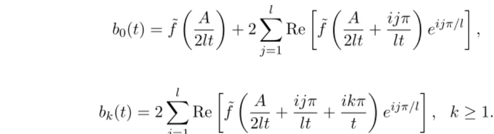
(48) E( ¯m, n) =sn(t) + ¯ m X k=1 ¯ m k 2−m¯sn+1:n+k(t), where, (49) si:j(t) = j X k=i (−1)kak(t), i < j, sn(t) =s0:n(t), with, (50) ak(t) = e A/2l 2lt bk(t), k≥0,

where, (51) b0(t) = ˜f A 2lt + 2 l X j=1 Re ˜ f A 2lt+ ijπ lt eijπ/l , and (52) bk(t) = 2 l X j=1 Re ˜ f A 2lt+ ijπ lt + ikπ t eijπ/l , k≥1.

The parameters l, ¯m and A are chosen to control the round-off and discretization errors of the approximation. Usually lis chosen equal to 1, so we consider l= 1. The parameter ¯m controls the round-off error in an inversely proportional way because the functions bk(t) in (52) are computed with a round-off error of 10−m¯. In our examples we take ¯m = 8 to achieve a round-off error of no more than 10−8. The parameter A controls the discretization error of the approximation and according to [9] the following relation provides efficient control of the parameters,

(53) A= 2l 2l+ 1 ( ¯mln(10) + ln(2lt)).

The remaining parameter nis the size of the partial sums.

We compare the WA approximation presented in Section 4.1 with the NLTI method. For this purpose, we plot the tail probabilities computed with both methods and we perform a MC simulation with 107scenarios for the systematic factor to get our benchmark distribution. The model considered is the simple one-factor Gaussian copula model (2) since this comparison is related only to the inversion step. The test portfolio has N = 50 obligors and shows severe exposure concentration E1 = E2 = 50, En = 1, n = 3, . . . , N. We consider Pn = 0.21%, ρn = 0.15, n = 1, . . . , N. The corresponding characteristic function is calculated as in [12], this is, following expression (8) for the one-dimensional case and solving the integral by means of Gauss-Hermite quadrature with 20 nodes. We plot the results in Figure 1. The left side plot of Figure 1 shows the tail probabilities obtained

0 0.05 0.1 0.15 0.2 0.25 0.3 0.35 0.4 0.45 0.5 Loss level 10-6 10-5 10-4 10-3 10-2 10-1 100 Tail probability WA NLTI MC

(a)WA (m= 10), NLTI (n= 350) and MC.

0.3 0.32 0.34 0.36 0.38 0.4 0.42 0.44 0.46 0.48 0.5 Loss level 10-6 10-5 10-4 10-3 10-2 10-1 100 Tail probability NLTI-n350 NLTI-n1000 MC

(b)NLTI (n= 350), NLTI (n= 1000) and MC.

Figure 1. Tail probabilities.

with the WA, NLTI and MC methods. The number of terms employed in NLTI is n= 350, while WA has been run at scale of approximation m = 10. We have made this choice of n in order to compare the accuracy of both methods at the same cost of CPU time2. We observe that while WA is capable to accurately approximate the benchmark solution, the NLTI method shows an oscillatory behaviour further in the tail, which may have an important negative impact in the computation of the ES. We zoom in to show in the right side plot of Figure 1 the approximation carried out by

2_{The programs are coded in MATLAB and run in a laptop with processor 2 GHz intel core i5 and memory 8 GB}

the NLTI method when considering more terms in the expansion. In particular, we represent the approximation with n = 1000 and observe that heavy oscillations remain in the tail. In addition to these oscillations, we underline the fact that there is not a prescription on the selection of the suitable parameter n, and adjusting its value may become a matter of trial and error. Regarding the selection made of the scale parameter m = 10 for the WA method it is worth remarking that, if we assume that coefficients cm,k in (39) were computed exactly, the true VaR value VaRα(L) would lie within the interval [₂¯km,

¯

k+1

2m] and would differ at most ₂m1+1 from the computed VaR value

l_αm = 2¯k+ 1

2m+1 following the algorithm explained in Section 4.2, since |VaRα(L)−l

m

α| ≤ 2m1+1. For

m= 10 we have ₂m1+1 ≈5·10−4, and we therefore expect (at most) three digits accuracy in terms of

absolute error with respect to the true solution. We take as a reference in this case a MC simulation with 107scenarios. The error is roughly proportional to√1

107 ≈3·10

−4_{, since this error is affected by}

the variance_√ pα(1−α) and the true density fL evaluated at the true quantile (see [7] for details), α(1−α)

fL(VaRα(L)) √

107.

5. Numerical examples

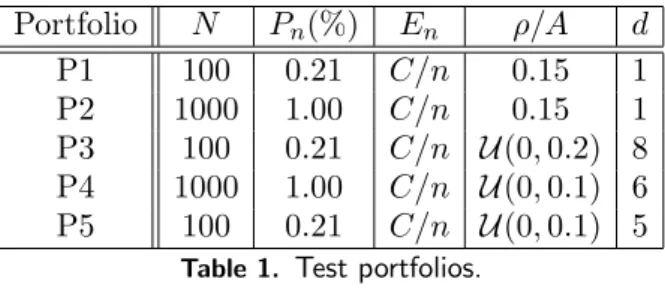
In this section, we show the performance of the WA method for a wide variety of portfolios when the firm-value is driven by the three different models presented in Section 2. The test portfolios are described in Table 1. The matrix A = (aij) for i = 1, . . . , N, j = 1, . . . , d contains the factor loadings associated to the models (4) and (13), that have been generated by simulation following a uniform distributionU(a, b). As pointed out in [10], the approximation of Section 3.1 works out well for moderate correlation among obligors, this is, when kAk is small, where kAk := maxjP

k|ajk|. The rationale behind is that the accuracy of the approximation depends on the goodness of the approximation (19). If paT

nan is small, then it can be seen from (17) that lngn(w, Sn) will be

almost linear in Sn and therefore (19) will fit better. In the extreme case where

p

aT

nan = 0,

lngn(w, Sn) becomes constant for all Sn and the approximation (19) becomes exact (a complete error analysis is presented in Section 3.2 of [10]). A remedy for the case of strong correlation is presented in [10]. The correlation parameter ρ in (3) is assumed to be constant for all the obligors in the portfolio. The dimension d = 1 refers to the model in (3). Observe that all test portfolios considered show name concentration andCis computed such thatPN

n=1En= 1. In all experiments of this section, we run the MC simulation with 106 scenarios for the systematic risk factors to estimate the VaR and ES risk measures at the regulatory 99.9% confidence level and write down those results as a reference. In regard to this point, we underline that for the reasons mentioned in the previous section, this is not a robust reference to compare with. A robust benchmark is to consider the average of a large sample of VaR and ES estimates with (for instance) 106 scenarios each rather than a unique estimate. We dismiss this last strategy because the computation time is in general unaffordable for the models presented in this work applied to portfolios P2 and P4. The wavelet-based approximation F_mc in (38) converges to the true distribution function Fc with the L2-norm when m increases, since Fc belongs to L2([0,1]). We therefore assume that the true solution is given by the WA method at scale m= 10 and use it as our benchmark.

The QTA approximation presented in Section 3.1 relies on the quadratic approximation of function g in (17) as well as on Proposition 1. This proposition can be applied when <(H) is negative-semidefinite and, as pointed out in [10], this is accomplished when γn(w) in (21) satisfies <(γn(w))≤0 for all n= 1, . . . , N. We carry out the computation ofαn(w), βn(w), γn(w) by means of weighted least squares and perform a linear approximation when <(γ_n(w)) is strictly positive. We look for αn(w), βn(w) and γn(w) that solve the minimization problem,

minX λ∈Λ ω(λ)ln (gn(w, λ))−αn(w)−βn(w)λ−γn(w)λ2 2 , <(γn(w))≤0.

The summands represent the approximation errors at certain grid points λ∈Λ, whereω(λ) repre-sents the penalty weight for the errors. We assume that Λ and ω are the same for all n and that

P

that variable Sn in (19) is a Gaussian distribution. For our numerical examples, we chooseω(λ) as exponentially decreasing in|λ|2, specifically, we chooseω to be the probability density function of a standard Gaussian normalized over Λ. While the grid points in [10] are chosen evenly between −3 and 3, we select the range −7 and 7, since our numerical experiments are more accurate within this interval. The advantage of using the least-squares method to determine αn(v), βn(v) and γn(v) is that the optimization problem has a unique closed-form solution.

Portfolio N Pn(%) En ρ/A d P1 100 0.21 C/n 0.15 1 P2 1000 1.00 C/n 0.15 1 P3 100 0.21 C/n U(0,0.2) 8 P4 1000 1.00 C/n U(0,0.1) 6 P5 100 0.21 C/n U(0,0.1) 5

Table 1. Test portfolios.

5.1. Multi-factor Gaussian copula. In this section we select portfolios P3 and P4 for the exper-iments. Figure 2 shows the tail probabilities compared to MC simulation. We name WA-QTA the numerical method employed, where WA stands for the inversion methodology based on wavelets and QTA refers to the quadratic transform approximation for obtaining the characteristic function, as explained in Section 3.1. 0 0.05 0.1 0.15 0.2 Loss level 10-4 10-3 10-2 10-1 100 Tail probability MC WA-QTA (a)Portfolio P3. 0 0.05 0.1 0.15 0.2 Loss level 10-4 10-3 10-2 10-1 100 Tail probability MC WA-QTA (b)Portfolio P4.

Figure 2. Tail probabilities.

We present the VaR and ES values obtained in Table 2 and the corresponding CPU time in Table 3. The risk measures can be obtained with less than 1% relative error at scalem= 9 in about one second for P3 and in about seven seconds for P4, where the dimensions are 8 and 6 respectively. We can get the risk measures in half of those CPU times at scale m = 8 keeping accurate results for VaR, although the accuracy worsens for ES.

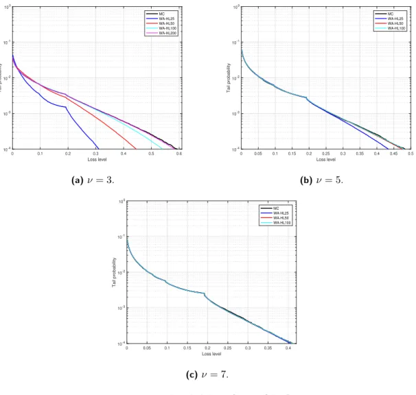
5.2. t-copula withν degres of freedom and t-distributed margins. In this section we select portfolios P1 and P2 for the experiments. We use the name WA-HLXX for the numerical method presented in Section 3.2.1, where H stands for Hermite, L stands for Laguerre and XX specifies the number of nodes considered for the generalized Gauss-Laguerre quadrature (nl). The number of nodes for Gauss-Hermite quadrature is fixed to nh = 20 for all experiments, as in [12, 14] for the one-factor Gaussian copula model. As in the previous section, WA-QTA refers to the numerical method presented in Section 3.2.2. Figure 3 shows the tail probabilities of portfolio P1 compared to MC simulation. We observe that the accuracy at high loss levels depends on the parameter ν, where a small ν requires a largenl and conversely.

Portfolio P3 Portfolio P4

Method VaR ES VaR ES

MC 0.1928 0.2029 0.1540 0.1718

WA-QTA (m= 10) 0.1948 0.2034 0.1558 0.1720

WA-QTA (m= 9) 0.1963 (0.8%) 0.1990 (2.2%) 0.1572 (0.9%) 0.1781 (3.6%) WA-QTA (m= 8) 0.2012 (3.3%) 0.2212 (8.7%) 0.1582 (1.6%) 0.2383 (38.5%)

Table 2. VaR and ES values at 99.9%confidence level for portfolios P3 and P4. The relative

errors at scales m = 8,9 with respect to the WA-QTA method at scalem = 10 are shown in

parenthesis.

Method Portfolio P3 Portfolio P4

WA-QTA (m= 10) 1.4 16.2

WA-QTA (m= 9) 0.7 7.2

WA-QTA (m= 8) 0.4 3.6

Table 3. CPU time measured in seconds for obtaining the VaR and ES values at99.9%confidence

level for portfolios P3 and P4.

0 0.1 0.2 0.3 0.4 0.5 0.6 Loss level 10-4 10-3 10-2 10-1 100 Tail probability MC WA-HL25 WA-HL50 WA-HL100 WA-HL200 (a)ν= 3. 0 0.05 0.1 0.15 0.2 0.25 0.3 0.35 0.4 0.45 0.5 Loss level 10-4 10-3 10-2 10-1 100 Tail probability MC WA-HL25 WA-HL50 WA-HL100 (b)ν= 5. 0 0.05 0.1 0.15 0.2 0.25 0.3 0.35 0.4 Loss level 10-4 10-3 10-2 10-1 100 Tail probability MC WA-HL25 WA-HL50 WA-HL100 (c)ν= 7.

Figure 3. Tail probabilities for portfolio P1.

We present in Table 4 results on portfolios P1 and P2 forν = 5 andnl= 50, and the corresponding CPU time is shown in Table 5. It is worth remarking that, as mentioned at the end of Section 4.3,

the theoretical absolute error estimate when computing the VaR valuelm_α at scalemis 1/2m+1. We observe that the theoretical error is in good agreement with the order of the empirical error at scale m= 9 when we compare with the benchmark at scalem= 10 since,

(54) |l10_α −l_α9| ≤ |VaR_α(L)−l10_α |+|VaR_α(L)−l_α9| ≤ 1 211 +

1

210 ≈0.001,

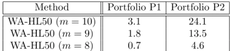
yielding a relative error of 0.001/26.81≈0.4% for P1 and 0.001/0.3970≈0.3% for P2. The CPU time is very competitive also for big portfolios like P2. Portfolios of this size are particularly difficult to handle by MC simulation.

Portfolio P1 Portfolio P2

Method VaR ES VaR ES

MC 0.2666 0.3562 0.3971 0.4817

WA-HL50 (m= 10) 0.2681 0.3569 0.3970 0.4913

WA-HL50 (m= 9) 0.2686 (0.2%) 0.3559 (0.3%) 0.3994 (0.6%) 0.5040 (2.6%) WA-HL50 (m= 8) 0.2715 (1.3%) 0.3596 (0.8%) 0.4004 (0.9%) 0.5305 (8.0%)

Table 4. VaR and ES values at 99.9%confidence level for portfolios P1 and P2. The relative

errors at scales m= 8,9 with respect to the WA-HL50 method at scale m = 10are shown in

parenthesis.

Method Portfolio P1 Portfolio P2

WA-HL50 (m= 10) 3.1 24.1

WA-HL50 (m= 9) 1.8 13.5

WA-HL50 (m= 8) 0.7 4.6

Table 5. CPU time measured in seconds for obtaining the VaR and ES values at99.9%confidence

level for portfolios P1 and P2.

In order to check the accuracy of the QTA method, we run this approximation at scalem= 10 for portfolio P1 using 50 nodes of generalized Gauss-Laguerre quadrature for the integral in (31). The results obtained are 0.2671 for the VaR and 0.3540 for the ES. The CPU time is 85.2 seconds. We get accurate results in comparison with the WA-HL50 method at the same scale of approximation, although the computational effort in this case is almost 30 times higher.

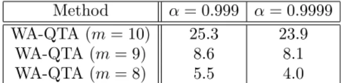
5.3. Multi-factor t-copula model. We consider in this last section the most challenging case among the three models presented in this work. We perform our experiments with portfolio P5 of dimension 5, we assume that ν = 7 and consider 25 nodes of integration for generalized Gauss-Laguerre quadrature in (32). We plot tail probabilities in Figure 4, where WAm-QTALjstands for WA-QTA method at scale of approximation m and using j nodes of generalized Gauss-Laguerre quadrature. We plot as usual MC as a reference and we observe highly accurate VaR values at scales m = 8,9 with respect to the benchmark scale m = 10 both at 99.9% and 99.99% levels. These results are confirmed looking at VaR values in Table 6. The ES values are very accurate at the regulatory level 99.9% and less accurate (but still competitive) values are obtained further in the tail at level 99.99%. It is worth mentioning that this high confidence level is particularly very demanding when computed by MC simulation. The CPU times are presented in Table 7. We highlight the impressive CPU times (measured in seconds) in particular at scales m= 8,9.

6. Conclusions

In this work we have investigated two highly efficient numerical methods to obtain the VaR and ES values for portfolios with exposure concentration under multi-factor Gaussian and t-copula models. It is well-known that MC methods are highly demanding from the computational point of view when dealing with big sized and high-dimensional models for the estimation of VaR and ES values at high confidence levels.

0 0.05 0.1 0.15 0.2 0.25 0.3 0.35 Loss level 10-4 10-3 10-2 10-1 100 Tail probability MC WA10-QTAL25 WA9-QTAL25 WA8-QTAL25

Figure 4. Tail probabilities for portfolio P5.

α= 0.999 α= 0.9999

Method VaR ES VaR ES

MC 0.2105 0.2613 0.3359 0.3886

WA-QTA (m= 10) 0.2114 0.2595 0.3267 0.3697

WA-QTA (m= 9) 0.2139 (1.2%) 0.2579 (0.6%) 0.3271 (0.2%) 0.3513 (5.0%) WA-QTA (m= 8) 0.2168 (2.5%) 0.2651 (2.1%) 0.3301 (1.1%) 0.4177 (13.0%)

Table 6. VaR and ES values for portfolio P5. The relative errors at scalesm= 8,9with respect

to the WA-QTA method at scalem= 10are shown in parenthesis.

Method α= 0.999 α= 0.9999

WA-QTA (m= 10) 25.3 23.9

WA-QTA (m= 9) 8.6 8.1

WA-QTA (m= 8) 5.5 4.0

Table 7. CPU time measured in seconds for obtaining the VaR and ES values for portfolio P5.

These two methods are called WA-HL and WA-QTA and they are composed of two main parts. The first part is the numerical computation of the characteristic function associated to the portfolio loss variable. We tackle this part by different techniques depending on the underlying model. For the (bivariate) t-copula model we perform a double integration with Gauss-Hermite and generalized Gauss-Laguerre quadrature and call this method WA-HL, while the multi-factor Gaussian model is treated with the QTA method put forward in [10] and called WA-QTA. The characteristic function for the most challenging model, this is, the multi-factor t-copula, is derived by conditioning on the chi-square random variable of the model and computed by applying the QTA method at each discretization point of the resulting one-dimensional integral. This last model is by far the most involved in terms of computing effort. Once the characteristic function for the loss variable has been obtained then the second part of the procedure comes into play. This second step is the Fourier inversion method called WA, which is based on Haar wavelets and it was developed in [12, 14] to recover the CDF of the loss variable. We have improved the efficiency of the WA method by computing the coefficients of the expansion by means of an FFT algorithm and we have shown that this method outperforms the NLTI inversion method in terms of efficiency and robustness.

The overall CPU time of the numerical methods employed is impressive taking into account their size and dimension as well as the confidence levels considered. This may be the first time that multi-factor t-copula model is considered outside the MC framework. This research opens the door to calculate the risk contributions to the VaR and ES risk measures under the same model assumptions and we will consider this problem in our future work.

Acknowledgment

The research leading to these results has received funding from La Caixa Foundation. G. C.-P. acknowledges AGAUR-Generalitat de Catalunya for funding under its doctoral scholarship pro-gramme. G. C.-P. and L. O.-G. acknowledge the Spanish Ministry of Economy and Competitiveness for funding under grants ECO2016-76203-C2-2 and MTM2016-76420-P (MINECO/FEDER, UE).

References

[1] J. Abate, G.L. Choudhury, and W. Whitt. An introduction to numerical transform inversion and its application to probability models.In Computational Probability, ed. W.K. Grassman, Kluwer, Norwell, MA, 2000.

[2] J. Abate and W. Whitt. Numerical inversion of Laplace transforms of probability distributions.ORSA Journal on Computing, 7(1):36–43, 1995.

[3] J.C.C. Chan and D.P. Kroese. Efficient estimation of large portfolio loss probabilities int-copula models.European Journal of Operational Research, 205:361–367, 2010.

[4] I. Daubechies.Ten lectures on wavelets. Society for Industrial and Applied Mathematics, 1992.

[5] F. Fang and C.W. Oosterlee. A novel option pricing method based on Fourier-cosine series expansions. SIAM Journal on Scientific Computing, 31(2):826–848, 2008.

[6] P.-W. Fok, X. Yan, and G. Yao. Analysis of credit portfolio risk using hierarchical multifactor models.Journal of Credit Risk, 10(4):45–70, 2014.

[7] P. Glasserman.Monte Carlo methods in financial engineering. Springer, 2003.

[8] P. Glasserman, W. Kang, and P. Shahabuddin. Large deviations in multifactor portfolio credit risk.Mathematical Finance, 17(3):345–379, 2007.

[9] P. Glasserman and J. Ruiz-Mata. Computing the credit loss distribution in the Gaussian copula model: a com-parison of methods.Journal of Credit Risk, 2(4):33–66, 2006.

[10] P. Glasserman and S. Suchintabandid. Quadratic transform approximation for CDO pricing in multifactor models.

SIAM J. Financial Math., 3(1):137–162, 2012.

[11] W. Kang and P. Shahabuddin. Fast simulation for multifactor portfolio credit risk in the t-copula model. In

Proceedings of the 37th conference on Winter simulation, pages 1859–1868. Winter Simulation Conference, 2005. [12] J.J. Masdemont and L. Ortiz-Gracia. Haar wavelets–based approach for quantifying credit portfolio losses.

Quan-titative Finance, 14(9):1587–1595, 2014.

[13] A.J. McNeil, R. Frey, and P. Embrechts.Quantitative risk management: concepts, techniques and tools. Princeton University Press, 2015.

[14] L. Ortiz-Gracia and J. J. Masdemont. Credit risk contributions under the Vasicek one-factor model: a fast wavelet expansion approximation.Journal of Computational Finance, 17(4):59–97, 2014.

[15] L. Ortiz-Gracia and J. J. Masdemont. Peaks and jumps reconstruction with b-splines scaling functions.Journal of Computational and Applied Mathematics, (272):258–272, 2014.

[16] L. Ortiz-Gracia and C.W. Oosterlee. Robust pricing of European options with wavelets and the characteristic function.SIAM Journal on Scientific Computing, 35(5):B1055–B1084, 2013.

[17] A. Owen, J. Bryers, and F. Buet-Golfouse. Hermite approximations in credit portfolio modeling with probability of default-loss given default correlation.Journal of Credit Risk, 11(3):1–20, 2015.

[18] M. Pykhtin. Multi-factor adjustment.Risk, March:85–90, 2004.

[19] M. Rutkowski and S. Tarca. Regulatory capital modeling for credit risk.International Journal of Theoretical and Applied Finance, 18(5):1550034,44 pages, 2015.

[20] L. Schloegl and D. O’Kane. A note on the large homogeneous portfolio approximation with the Student-t copula.