Fat Products
Alexei Alexandrov Northwestern Universityy
November 20, 2006
Abstract
The economics literature generally considers products as points in some characteristics space. Starting with Hotelling, this served as a convenient assumption, yet with more products being ‡exible or self-customizable to some degree it makes sense to think that products have positive measure. I develop a model where …rms can o¤er interval long ‘fat’ products in the spatial model of di¤erentiation. Contrary to the standard results pro…ts of the …rms can decrease with increased di¤erentiation - there is a standard e¤ect of lowering the incentive to cut prices, but there is also an incentive to provide more content sometimes resulting in lower pro…ts. Consumer welfare increases unambiguously with respect to the standard model of Salop. I also …nd that it is pro…table for …rms to commit as an industry not to make fat products. If one …rm is a leader and another is a follower, the leader accommodates the follower by settling for less pro…ts if di¤erentiation is small.
1
Introduction
Harold Hotelling was arguably the …rst to introduce product di¤erentiation. In his model a prod-uct is a point in the linear space of characteristics. While that model is generally associated with di¤erentiation in locations and distances, it is clear from the article that Hotelling had character-istics space in mind – he talks about how his model applies to things from sweetness of cider to
I would like to thank Daniel F. Spulber for advising me throughout the process of writing this paper, and in particular for a great title for the work. Martin Lariviere and Alberto Salvo spent many hours discussing this paper and pointing out works I have not looked at yet. I would also like to thank Anne Coughlan, George Deltas, Johannes Horner, Scott Stern, Tom Hubbard, and Alessandro Pavan for their valuable comments.
political parties’ positions on tari¤s. Lancaster’s work (1971) formally extended the de…nition of the product to a point in some characteristics space with many dimensions of di¤erentiation, while giving credit to Hotelling for being the pioneer in the …eld:
Hotelling had provided a hint as to a possible solution of the product variation problem by extending his model of pure spatial competition. . . Hotelling himself did not develop the idea further, Chamberlin ignored it, and no one else took it up.1
A product is generally de…ned as follows: "a complete bundle of bene…ts or satisfactions that
buyers perceive they will obtain if they purchase the product."2 Why should we think of a product as
a point in a characteristics space? Since Hotelling’s article, the economic literature has represented products as points. This has proved to be a useful and convenient assumption that stood the test of time. The following question arises, however: "why should consumer’s utility function be de…ned just over points?" A general de…nition of a product should have utility maps going from a set of characteristics to the real line. If we want to look at maps that are relatively better behaved, then we can look at maps of “contiguous” sets of characteristics – intervals in one dimensional Hotelling space. The cost function of the products can also be a map from the set of the product’s characteristics to the real line. If results turn out to be broadly similar to those using utility and cost functions de…ned over points, then we can safely continue using the latter assumption. Otherwise, more general de…nitions are needed.
In this article, I examine a straightforward extension of point products to interval-long products in a one-dimensional spatial model. I refer to these as "fat products". A consumer’s utility depends on whether or not her preferred point is inside the range of the product. If it is, then the consumer does not need to incur any travel or adjustment costs3. If it is not, then the consumer has to incur the costs of traveling to the border of the product. As a result, …rms can position their product closer to some consumers without moving away from others. However, such ‡exibility is costly –a …rm’s cost of developing a product is a convex function of the length (measure) of the product.
I …nd that the …rms would be willing to collude to make zero measure (point) products, but in the absence of collusion they develop products of positive measure. Moreover, …rms might
1See Lancaster (1971), p. 16 2
Wikipedia (English), search query "product".
3I will go on referring to travel or transportation costs throughout the article, although costs of adjustment to a
incur losses as the degree of di¤erentiation increases, because while in equilibrium prices rise, the equilibrium range of the product rises as well, in several instances resulting in an overall drop in pro…ts. As a consequence if there is a free entry (or zero pro…t) condition, this would imply that as the market grows, or becomes more di¤erentiated, the number of …rms that can survive stays constant or even decreases, as each …rm unilaterally …nds it optimal to escalate its R&D spending and increase the measure of its product.4
I examine an extension, in the spirit of Stackelberg competition, where there are two …rms, and one of them is a leader – it picks the price and the size of her product …rst. I …nd that with su¢ ciently small development costs the leader picks bigger price and measure than the follower, and ends up with higher market share and pro…ts as one would expect. However, the result is reversed if the development costs are bigger (or the …rms are more homogenous) –the leader accommodates the follower by picking a smaller measure than the follower will, and under some conditions even charging smaller price.
There are several branches of literature close in appearance to Fat Products. One of the most well-known is bundling. Bakos and Brynjolfsson (1999) examine bundling of many goods, with the application discussed being distribution of digital goods via internet. The model is built on the law of large numbers, and the assumption that consumers’ valuations are i.i.d. The outcome is that bundling a very large number of products can be pro…table because the …rm can just charge the mean of the distribution. The bundling literature had focused on independently valued products and occasionally on complements. One of the very few articles on bundling of substitutes is by Venkatesh and Kamakura (2003) which …nds that if the goods are highly substitutable, it is not a good idea to bundle to them. The interval-long products in the Hotelling space with each consumer interested in her ideal point can be viewed as a bundle, however it is a bundle of an uncountable number of goods (all the points in the Fat Product), where the value of the bundle is the value of the most valuable good in that bundle.
My model also has some similarity to articles describing the "crowding out" e¤ect, in particular to Schmalensee (1978). While the intuition from that article is that incumbents …ll up the whole 4This "escalation mechanism" is reminiscent of Sutton (1991). As …rms’willingness to pay for broader products
increases, Sutton’s escalation mechanism kicks in. Related to this idea is recent work by Ellickson (2005) looking at supermarkets as natural oligopolies in terms of making their product o¤erings broader, the stores larger, and the aisles wider, therefore not letting in more …rms as the market size grows.
arc of a circle, they do it for deterrence reasons. In my model, where there is no deterrence, …rms …ll up intervals to capture more consumers not worrying about potential entrants. The extension with a leader and a follower has some resemblance to Schmalensee results if the costs of development are not too high – the leader will choose to produce a product of big measure and force the follower into a market niche. Of course the products are still point products in Schmalensee (1978), which may make more sense as far as cereal is concerned.
Cheng and Nahm (2006) examine what happens in a vertical di¤erentiation model when there is a system of a base product and an add-on which is valueless by itself. As the value of the base product increases, keeping the value of the system constant the pricing will go from comple-mentary with the double marginalization problem to independent getting rid of the problem. My model examines the optimal boundary of products in the horizontal di¤erentiation framework with competing symmetric …rms.5
2
Applications
Here is how Gerard Debreu describes a product ("commodity") in Theory of Value (1959):
a commodity is therefore de…ned by speci…cation of all its physical characteristics,
of its availability date, and of its availability location. As soon as one of these factors changes, a di¤ erent commodity results.6
Contribution of this article is to think of locations, characteristics, and dates as ranges as opposed to being points. Location does not have to be a point. A consumer can request a delivery, and then a product can be at a di¤erent location without resulting in a di¤erent product. If delivery costs the same in some area then wheat in Chicago and wheat in Minneapolis can be thought of as the same product. A trip on Chicago’s Elevated Line costs two dollars no matter if the customer goes one mile down the line to a store or some twenty miles from Evanston to Hyde Park7. If the consumer lives far from the end of a line, then she can walk or take a bus from the last stop, which will require extra expenses – just like the fat products model. In fact, any access good can be
5Discussion of other related literature is scattered throughout more relevant (for a speci…c article) sections. 6
Debreu (1959), page 30. Italics are preserved from the original.
7
thought of as a Fat Product. Consumers pay to access the good and pick what they want inside – the applications range from Disneyland to network access to all-you-can-eat bu¤ets. The measure of the product is then the extent of the access provided.
Imagine a beach and two vendors selling ice-cream. Instead of being stationary they can walk around, and the consumers who are not in one of the route intervals (or who are dissatis…ed with the price in the route they belong to) can come to the boundary of one of the routes and wait for the vendor to come by. I am interested in how long are the vendors’ routes, and what price will they charge. Alternatively, two vendors can be at the opposite ends of the unit interval, deciding how much extra ground to cover (or maybe to just stay in one place if the optimum is zero)8.
I do not intend the model to just be a spatial model –this is a model of product di¤erentiation. Think of an o¢ ce chair. One can adjust height up and down in a continuous interval – each …rm does not have many lines of otherwise the same o¢ ce chairs, each of a particular height. Think of how much sugar you put in your co¤ee for the same price. Sweetness of cider was one of Hotelling’s applications, but if you come to the co¤ee shop and the sugar is free, then you can continuously adjust the sweetness to your own taste without paying more. Brightness and focus of a projector or a TV set, self-customizable products, and all of the above are examples of fat products. The consumer gets an interval of characteristics in one product, and can pick the one that she wants. Another example to look at is any software with options. The user can adjust how big is the window, the size of the font, the color of the letters – whatever that software specializes in, but still the available characteristics to the user are an interval of characteristics (i.e. how wide should the window of Acrobat Reader be –from zero to the width of the screen), for which the user does not have to pay more.
Lancaster in his book had provided another kind of application for fat products with respect to characteristics –combinable goods.
If goods are combinable, so that two goods can be consumed simultaneously to give a characteristics collection that is a combination of the characteristics of the separate goods.... the problem must be approached anew... In the combinable case, however, the individual could attain exactly the most-preferred collection of characteristics (that 8Thanks to Shane Greenstein for this example.
is the collection he or she would obtain from the most-preferred good, if it were available) by consuming goods Y and Z together.9
The fat products are combinable goods with the goods Y and Z being the endpoints of the interval, and bundle Y and Z sold by one …rm. Imagine buying a cocktail set – every consumer can make their own favorite combination while paying the same price, while the combination can vary continuously. Alternatively one can mix hot and cold water in the tap to achieve the perfect temperature. There is already some literature on the combinable goods, started by Anderson and Neven (1989), who prove that with combinable goods …rms end up playing the socially optimal strategies. The consumers in this literature can buy a bit of both products around them and mix them together, however these are point products being o¤ered by di¤erent …rms.10
An example with time for Fat Products is coupons that consumers can use in a given time period. The coupon does not change if it is used several days before or several days after, and the length of the product is just the expiration date of the coupon –then the value is zero. While the coupon loses the value after the expiration date, the companies issuing them still have to think over the length of the period when the coupon might be used.
Stores’operating hours is a close concept to a fat product – the consumer can go to the store at whatever time the store is opened without having to pay extra fees. Anyone checking in at a hotel can check in whatever time they want to in a given interval (say, from 4pm). Also operating hours are easily modeled as one-dimensional and intervals –it is hard to imagine a store or a hotel opening and closing for a few seconds each minute.
Shopping hours literature developed some models close to interval-long products in one dimen-sional space. The shops are picking the hours when are the stores open and prices. Consumers have optimal shopping times and incur disutility if they have to move their shopping hours if the store is closed at a particular time.11 The literature is mainly interested in what happens if the
9
Lancaster (1971), p. 56–58.
1 0The applications of this concept are TV viewing and advertisement, where viewers can see di¤erent channels in
the same day, and pick the optimal mix for them. Two recent papers on the topic are Gal-Or and Dukes (2003) arriving at a conclusion that …rms prefer to minimally di¢ rentiate their products and Gabszewicz et. al. (2004), where the authors …nd that the less viewers like advertising the closer will the TV stations come to eachother .
1 1
Inderst and Irmen (2005) considers two shops choosing between being opened either at day, at night, never or always. The result is that there can be some asymmetric hours provision from two ex-ante similar stores. Also, if shopping hours are regulated, the retailers will charge higher prices and will be better o¤. Shy and Stenbacka (2006) considers continuous time intervals, yet keep prices as exogenous, again resulting in the possibility of asymmetric shopping hours, and in the fact that shops are not opened long enough from the social welfare point of view.
government regulates the shopping hours, and when is it possible to set asymmetric opening and closing hours, but while asymmetric distribution of consumers plays a big role in that literature, this model might still be useful in that context.
3
Monopoly
3.1 The Fat Products Monopolist Model
The model setup closely follows that of Salop, with the important di¤erences in the parts describing the production possibilities and costs. The conceivable goods are located along the unit interval. The consumers are going to be the standard address consumers –located uniformly along the unit circumference circle, with some …xed reservation price for the product, sayR >0, and transporta-tion costst d–withd 0being the distance between the consumer and the product12, andt 0
being the marginal cost of transportation. If the consumer has a choice, she is going to buy the product to maximizeU(d) p, wherepis the price of the product, andU(d) =R td. The outside option’s utility is0.
The monopolist can choose to make products in a form, and with the characteristics of an inter-val, say[a; b],0 a b 1, with the development/production cost of a productCdevelopment([a; b]) = c(b a), where c( ) is a function. I will usually refer to the length of the interval o¤ered as m13. The standard measure zero products will be developed/produced with some positive …xed cost, so
c(0) = F > 0. Also let c0(0) = 0 to avoid the uninteresting case where the costs are so steep to expand from a point that no …rm will be willing to take them. I will assume throughout the paper
thatt > R, i.e. in the simple monopoly case there are consumers who do not buy the good.
3.2 Non-Negative Measure Solution
To make sure that the second order conditions are satis…ed I make the following assumption14.
Su¢ ciently Convex Cost Assumption (M).Let the cost functionc(m)of developing/producing
a fat product of length m be such that c00(m) t
4.
1 2or the closest point on the interval in case of the product being an interval 1 3
U for Utility, tfor Transportation,Rfor Reservation,cfor Cost andmfor Measure
1 4For an example where this assumption is not satis…ed (the costs are linear) and consumers are on a unit interval
Does this assumption make sense? Since c is a cost function, it should be increasing. This assumption requires the cost function to be not just convex, but also have the second derivative bounded away from zero. Since adding an extra" >0of measure to the product requires this "to interact with the rest of the measure already in place, it seems natural to assume that as measure increases the addition of the same " becomes more and more costly. Now we can move on to the proof.
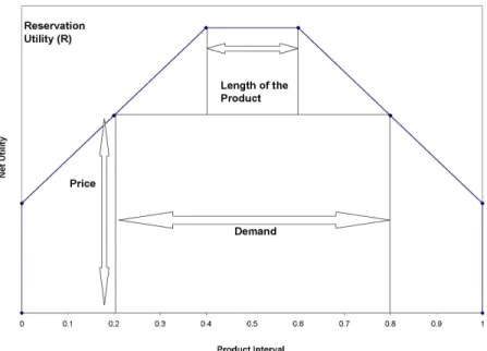
Figure 1. Consumers’utility with a Fat Monopolist.
Theorem 1 (Fat Product Monopolist). A monopolist which has the ability to o¤ er a Fat Product
charges p = R
2 +
tm
4 and makes products with the measure of m , such that c
0(m ) =p .
Proof. The di¤erence between the …gure above and a standard spatial problem is that before the
net utility (utility less the travel costs) would look like a triangle as opposed to a top of a trapezoid –there would be no ‡at part. The demand remains from the zero measure case, but there is also a portion added, equal to the length of the Fat Product. Therefore the demand for a given price for a non-negative length measure m will beD(p) =m+ 2(R p)
t .
Therefore the pro…t of the monopolist will be M+(p; m) = p D(p) c(m) = p(m+ 2R
2p2
t c(m).
I need to look at the Second Order Conditions to make sure that the function is concave in
p and m. The Hessian is HM(m; p) =
2 6 4 4 t 1 1 c00(m) 3 7
5. To ensure concavity the …rst leading principle major needs to be less than zero, and the determinant needs to be positive. The …rst leading major is 4=t, and sincet >0it is negative. Looking at the determinant, we can see that the second order conditions are satis…ed i¤c00(m) t
4.
Now look at the First Order Conditions:
@ @p =m + 2R t 4p t = 0 =) p = R 2 + tm 4 . (1) @ @m =p c 0(m ) = 0 =) c0(m ) =p . (2)
3.3 Comparing the Results
Notice that if we force m = 0, we get the results that we would have with the standard point products (p0 = R
2). The optimal measure is increasing in both R andt, which is intuitive as if the
utility to be extracted from the consumers is high, the monopolist will o¤er a wider product, and if the transportation costs are higher, then the incentives to o¤er a wider product increase.
Note that the condition on the derivative of the cost function is exactly the marginal revenue equals the marginal cost condition. Increasing the measure by an epsilon increases the demand by epsilon, and therefore the revenue by epsilon times price. But increasing the measure by an epsilon costs the derivative of the cost function at the current measure times epsilon.
The prices are higher with a fat product since not only does the …rm need to cover the devel-opment costs, but also now they can extract the full reservation price. The pro…ts are of course higher as well, since measure equal to zero option was there for the …rm to take. It is not obvious what happens with the number of the consumers served, and their welfare.
standard assumptions.
Proof. D(p ; m ) = m
2 +
R
t > D(p0).
The e¤ect of Fat Products on consumption is unambiguous - even though the price is going up, the more of the measure o¤ered, the more product is going to be sold. It is not as straightforward for the consumer welfare.
Proposition 1 Consumer welfare will increase under Fat Products i¤ R > 3tm
4 .
Proof. Consumer welfare is the trapezoid above the price line and below the net utility curve on
Figure 1. Therefore, its area is easy to calculate: CW+=
(D +m ) 2 (R p) = R2 4t 3tm 2 16 + m R 4 .
Compare this to the consumer welfare with m = 0, which is CW0 =
R2 4t. CW+ > CW0 i¤ 3tm 2 16 + m R 4 >0or equivalently R > 3tm 4 .
The result says that as R increases it is easier for the consumer welfare under Fat Products to be bigger than under the measure0case. This happens because all the consumers who are getting exactly what they want (i.e. located within the product interval) are getting much more utility than in the standard case even if the price is slightly higher, and increasingRincreases all of their utilities more than it would under the standard case. As for the result in m , since the optimal measure is directly related to price, it is clear that as the measure increases, so does the price, and the welfare must decrease with respect to the measure0 case. When the transportation costs increase, so will the price, as opposed to the standard case, and again the welfare will decrease comparatively.
Notice that we need the su¢ ciently convex cost assumption to make sure that the SOCs are satis…ed, however if the assumption does not hold, the equilibrium might still exist. In the Appendix A I derive the equilibrium for linear costs of expanding the measure and the customers located at the unit interval. Both of these make the proof much harder and do not add much intuition to the result. The results are that if the cost of the expansion is low enough then the monopolist will cover the whole interval and chargep=R, leaving consumers with0 welfare. Otherwise the monopolist goes back to the standard point product.
4
N Firms in Bertrand Competition
4.1 Introduction and Setup
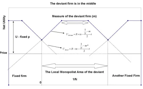
I am going to solve the N …rms problem, competing a0la Bertrand. A given …rm will take the prices and the measures by the other …rms as …xed. The …rms and the consumers will be in a circular city. For the local analysis I will use three …rms on the unit interval –with the two …xed …rms and the deviant …rm, the prices and measures of the …xed …rms …xed and equal. To provide intuition behind the math, the …gure on the next page is provided. To make the matters even simpler, the reader can view this as a duopoly along the circumference competition – since the prices by the other …rms are …xed, then it does not matter whether there are two …xed one side …rms, or one …xed …rm on both sides.
4.2 Fat Products versus Multi-Products
There is a big literature on Multi-Product …rms – the ones which can make several products and price them accordingly15. The reasons not to make many points instead of an interval are …xed costs and economies of scale. Think of the two ice-cream vendors from the application section. Would it make sense to put dozens of stationary vendors instead? Probably not, because of the …xed cost of hiring each additional vendor. For the same reason, and economies of scale, it would not make much sense to develop dozens of chairs of di¤erent heights or several projectors of di¤erent brightness and focus which are otherwise the same. The literature on product lines and mass customization moves in similar direction as the Multi-Product …rms literature. The bene…t of an adjustable good versus a mass customized line of goods is still in …xed costs and economies of scale. Here is an example to illustrate this point from Zipkin’s (2001) discussion on the limits of Mass Customization.
...there was talk of customizing car seats. Toyota even set up a prototype of a seat-measurement device at its visitor center in Toyota City. It never happened. Instead, adjustable seats developed rapidly. It is cheaper to construct adjustable seats than to customize.
1 5
If the …xed cost F of producing a point product is high enough, no …rm would be willing to make two of them. The conditions on when does it cost less to produce one fat product or two endpoints of the product are easily derived16. What happens if the …xed costs go to zero, and the …rms would prefer to make many point products? Then if there is more than one …rm, we have the result due to Teitz (1968) that there does not exist a pure strategy Nash equilibrium where …rms can choose to produce more than one product with linear travel costs for consumers. I will examine the oligopoly structure as if there is no option to develop more than one product –or that the …xed costF is high enough.
Think of a belt –it has many adjustment positions (holes), but the adjustment is not continuous. This is not a multi-product o¤ering. This is a fat product, where instead of an interval, the product is a set of multiple points. All the results hold the same, except for consumer welfare –the consumers whose favorite position is between two holes of the belt will get less welfare than with an interval. However, as long as there are a few points inside the interval, these consumers will not be marginal, therefore many points as one set as opposed to an interval only will matter for quantitative results on consumer welfare, while all the other results (including qualitative on consumer welfare) will go through as is now.
4.3 The Fat Products Oligopoly Model
The model setup is almost the same as that of Section 3, except that now there areN …rms located symmetrically around the unit circle, and the products are arcs on the circle. The consumers are going to be the standard address consumers –located uniformly along the unit circumference circle, with some …xed reservation price for the product, sayR >0, and transportation costst d–with
d 0 being the distance between the consumer and the product, and t R being the marginal cost of transportation. If the consumer has a choice, she is going to buy the product such that to maximizeU(d) p, wherep is the price of the product, andU(d) =R t d.
The producers can choose to make products in a form, and with the characteristics of an interval (so an arc, since it is a circular city), say[a; b],0 a b 1, with the development/production cost of a product C([a; b]) =c(b a), wherecis a function. I will still refer to the length of the interval
1 6
c(m)<2F, or equivalently the additional cost of developint a positive length product must be less than the …xed cost.
o¤ered as m. The standard measure zero products will be developed/produced at some positive …xed cost, so c(0) =F > 0. Before proceeding with the proof, I need the following assumption to ensure that the second order conditions hold. The implications of the assumptions were discussed in the monopoly section. Notice that this bound is weaker than the one in the monopoly section, which makes sense since competition implicitly makes it harder for the …rm to expand its’measure further.
Su¢ ciently Convex Cost Assumption (N).Let the cost functionc(m)of developing/producing
a fat product of length m be such that c00(m) t
8.
I only focus on pure strategy symmetric Nash Equilibria as the solution concept. Consider what happens if some consumers are left out of the market.
Lemma 1 (Full Coverage Lemma). The only equilibrium such that there are consumers left out of
the market is the trivial equilibrium where the global monopolist’s problem is the same as the local monopolist’s problem.
Proof. See appendix B.
In this case the scaling up of the market is not valid, since as N goes up and everything else stays constant this equilibrium will eventually disappear, and it will be harder and harder to let every …rm to optimize as if it is unconstrained by the neighbors. From now on I will assume that the parameters do not lead to the trivial case where a …rm can act as a global monopolist, and move on to the case where there are no consumers are left out of the market.
4.4 No Consumer Left Out
Now that there are no consumers left out, we can use Figure 3 (see below). First, I need to examine the possibility of a price equals marginal cost equilibrium. The price equal to marginal cost situation can arise in the case where no consumer is left out if either all the …rms produce measure 1/N products, or if all of them produce measure zero products. In either case, a deviant …rm can unilaterally raise its price above zero. This will clearly bring in positive pro…ts, and so we can not have a zero pro…t equilibrium in my model, unless one includes …xed costs of entry in the industry. To make sure that the …gure below looks right, I need to show that products of competing …rms do not intersect.
Lemma 2 There is no symmetric Nash equilibrium where products of two …rms intersect.
Proof. See appendix B.
In the main proof below I …x all the …rms’ measure and prices at the same level, and check whether a deviant …rm has an incentive of moving away from the knife-edge equilibrium where the local markets just touch, andp > c(m ).
Figure 2. Oligopoly with Fat Products.
Theorem 2 (The N-Firm Fat Product Competition). In the symmetric Nash equilibrium of N
…rms capable of o¤ ering fat products, each …rm charges p = t
N and makes a product with the
measure m < 1
N, such that c
0(m ) = t
2N (The Optimal Measure Condition).
Proof. (For details the reader is encouraged to look at Appendix B).
Fix the measure and the price of the …xed …rms at m and p , and denote by m and p the measure and price of the deviant …rm with respect to which it is going to maximize its’pro…t.
First, I …nd the demand function –which is determined by the marginal consumer –who is at the intersection of twoU(x)functions (on Figure 2 above), one of the consumers buying a deviant …rm product, and the other one of the left Fixed …rm. Just making the two equal to each other,
the intersection point is x(m; p) = m m
4 +
p p
2t , so if the deviant …rm lowers the measure of
its’fat product,m, the intersect point will move to the right, cutting into deviant’s market share. Raising price p has the same e¤ect. Since the deviant …rm competes with two …xed …rms, one on each side, the demand for the deviant …rm isDdeviant(m; p) = 1
N 2x(m; p), and the pro…t is then deviant(m; p) =DA(m; p) p c(m).
To insure that the Second Order Conditions hold, use the Su¢ ciently Convex Cost assumption. Then using the First Order Conditions together with symmetry (m=m ,p=p ), get the optimal pricep= t
N, and the optimal measurem , which, if an interior solution, has to satisfy the Optimal
Measure Condition: c0(m ) = t
2N, and cannot be outside of the interval[0;
1
N).
Then to …nd the pro…t simply substitute the optimal values into the objective function, and the consumer welfare is N times the area of the trapezoid in the deviant …rm region in Figure 2.
Corollary 2 In the symmetric equilibrium each …rm will get a pro…t of + =
t
N2 c(m ), and
the consumer welfare is going to be CW+=
1 +N +m
2 (R
t
N).
5
Comparison with Previous Literature
5.1 Summary of the Results
I considered two cases in the previous section. The trivial case equilibrium, with some consumers left out, happens when the local market optimization is the same as the global one, so the …rms do not have an incentive to deviate even if the ex-post markets are expanded. We get N local monopolists, with strategies described in Section 3.
In the more interesting case, the market is covered, and the second order conditions are satis…ed if the cost function of the measure of the product is su¢ ciently convex. I will focus on this scenario for the rest of the paper. Prices are the same as in Salop, pro…ts are lower and consumer welfare is higher. The measure o¤ered by …rms in equilibrium is sometimes positive, and depends on the exact form of the cost function. This is intuitive and something that we would expect from the monopoly results.
5.2 Comparison with Salop
Corollary 3 The equilibrium price is the same, the pro…ts of the …rms are lower, and the consumer
welfare is higher in the Fat Products oligopoly than in the standard oligopoly equilibrium.
To see the results of Salop one can just substitute m = 0 into the results of Theorem 2 – the fat products model is a generalization of Salop’s model. The price is the same, which is the most unexpected result, especially after Theorem 1, where in the monopoly case the price charged was higher than the standard. The prices remain the same since what determines the prices is the slopes of the net utility curves at the marginal consumer (the intersection). Those remain the same as they were in Salop’s model. Clearly this result is due to the assumption of linear travel costs. Pro…ts are lower since there is the extra cost of providing fat products, while the revenue stays the same. The consumer welfare went up since in the Salop equilibrium the welfare would just be N
triangles with bases of 1
N and heights of reservation price less the actual price. Now we have N
trapezoids, and as long as the measure is positive consumer welfare goes up. In the limit case of measure being equal to one the consumer welfare will double.
The more …rms there are in the industry, the overall pro…ts can actually become higher. Whether it happens depends on the exact form of the cost function. This possibility arises because the diseconomies of scale issue in the cost of fat products is becoming less severe as N increases.
If we look at the …xed cost, like Salop did, the …xed cost in this industry to support a SPZE (sub-game perfect zero pro…t Nash equilibrium) would be less than the ones in the original model, since there is the cost of positive measure that the …rms have to pay now that they did not have to worry about before.
Corollary 4 It would be pro…table for all the …rms in the market to commit to making only m= 0
(standard) products.
Recall the example of two ice-cream vendors. What this corollary means is that they would rather agree that both of them stand as opposed to walking around and try to appeal to more consumers. The intuition behind this result is as follows. Since the prices and the demand are the same as in Salop, the revenues are the same as well. However, the …rms have to pay extra cost for making their products fat. There is an arms race which bene…ts in the end only the customers
-without the e¤ects of the competitors the …rms would happily make their products fatter, but with the competitors doing the same, fatter products only help the customers.
What happens to pro…ts if t goes up, or as the products become more di¤erentiated? Just looking at the equation + =
t
N2 c(m ) the immediate reaction is that they necessarily go
up. However m depends on t, and as t goes up, so does m . The following numerical example illustrates an interesting point.
Example 1 Let there be N …rms in the city. Let t2(6;8) and c(m) =em. Then the su¢ ciently
enough cost condition is satis…ed (since em 1 t
8 for m 0) and c(0) = 1 >0. Also let R be
close to t so that all the …rms being local monopolists is not an equilibrium.
Then c0(m ) = t
2N, and therefore c(m ) =
t
2N. Also notice that m = ln
t 6 0. Thus the pro…t is +(t; N) = t N2 c(m ) = t N2 t 2N = 2 N
N2 t. WithN >2 this decreases in t!
Therefore with the Fat Products we get the unexpected conclusion that pro…ts do not neces-sarily increase as the transportation costs go up! This is a clear di¤erence from the predictions of Salop (1979) since there we got a clear conclusion that the pro…ts will go up as the transportation costs (di¤erentiation between the products) go up, since there the pro…ts per …rm were simply t
N2.
Proposition 2 In equilibrium pro…ts will go down as the transportation costs go up (…rms become
more di¤ erentiated) if and only if c00(m )< t
4.
Proof. All is needed is the derivative of pro…ts with respect tot, however …rst we need to implicitly
di¤erentiate the Optimal Measure Condition with respect tot:
c00(m )@m @t = 1 2N =) @m @t = 1 2N c00(m ). (3)
Then di¤erentiate the pro…t function = t
N2 c(m ): @ @t = 1 N2 c 0(m ) @m @t = 1 N2 t 2N 1 2N c00(m ) = 4c00(m ) t 4N2c00(m ). (4)
To see when is pro…t going down with respect totwe now just need to check when is (4) less than zero. Since c( ) is convex by assumption, c00( )>0. Therefore @
@t <0 i¤c
00(m )< t
for the N …rm part of the paper we just needed to assume that c00(m ) > t
8, therefore the region
where both inequalities are satis…ed is not empty.
What is the intuition behind this surprising result? In Salop’s model the reason that the pro…ts go up with the increase in transportation costs is that now the rival …rms do not have as much incentive to lower their prices to undercut, since after undercutting not as many consumers are going to switch because of the travel costs. This gives the …rms the ability to price higher without fearing the competition.
Once again, recall the example with two ice-cream vendors. Suppose it becomes hotter, so the travel costs go up for the consumers. Then the vendors become more di¤erentiated, but the value of walking closer to a given consumer increases. Therefore under certain conditions the vendors will do more additional walking than the additional pro…ts that they will receive due to increased di¤erentiation. In this model there are two di¤erent e¤ects at play. First one is the one described above. The second one is that with increase in t expanding the measure of the product becomes more and more valuable way to attract consumers than it was before. And so instead of competition in prices, the …rms engage in cut-throat competition in content. In equilibrium it is clear that even though the …rms will o¤er more content, they will still attract the same number of consumers, therefore with increase intwe have a welfare transfer from …rm pro…ts to consumer welfare.
Why do the pro…ts not go down with t if the costs are very convex? This happens because if the costs are too steep they act as a deterrent for …rms to increase the measure too much, therefore this way the …rms actually bene…t from higher costs.
5.3 Comparison with Mass Customization
5.3.1 Setup
Mass customization in operations research is a model is of a base point product in the spatial model of di¤erentiation, and a …rm that can produce point products close by to the base product for a higher cost. The …rm can charge consumers di¤erent prices for di¤erent products. Dewan et.al. (2003) examines a duopoly with quadratic costs of making products away from the base product. The main results are that the duopoly would o¤er less scope of products than a two-facility monopolist, the prices stay the same as in Salop’s model, and that if the …rms do not enter
simultaneously, then the …rst entrant always achieves advantage. Mendelson and Parlakturk (2005) looks at a duopoly with a two stage game – in the …rst stage the …rms decide how much (if at all) to invest in mass customization, and in the second stage they decide on the pricing structure. The …ndings are that a …rm with either quality or cost disadvantage will not want to customize by itself, and that occasionally even free customization might hurt …rm’s pro…ts.
A branch of economics closely related to mass customization is product line competition. This literature concerns …rms which can o¤er several products for di¤erent prices. One of the …rst e¤orts is an insightful article by Klemperer (1992), which results are driven by customers having switching costs from one brand (or store) to another, and so the …rms would try to position their products next to each other, as opposed to the standard Hotelling intuition. One of the latest e¤orts is Draganska and Jain (2005) empirically examining the e¤ects of extending the product line (i.e. o¤ering new ‡avors of yogurts) when the customers have preference for variety. They …nd that the product line length and price are substitutes from the …rm’s point of view - if the …rm wants to increase the price and keep the market share constant it should increase the product line as well, which I …nd as well – if the …rm wants to increase the price, it needs to extend the length of the interval as well.
I will assume an exact functional form for the cost function and compare the results of the equilibrium from the previous section to the results obtained by Dewan et.al. for Mass Customiza-tion. The Mass Customization model has exactly the same setup from the consumers’side as the standard Salop and the Fat Products model. The di¤erence comes on the production side.
In Mass Customization, each …rm has a focus point – the standard product, and can produce a tailored product x units away from the focus point forc(x). In that article the authors assume a duopoly (soN = 2) with quadratic costs, with positive coe¢ cients on x2 and x (which makes it
easy to satisfy the Convex Enough Cost Assumption) and the constant being zero. The price of the goods listed is the price of the focus good, with the optimal price of a tailored good is the “base price” of the focus good plus the transportation cost from the focus good to the tailored good (i.e. if the focus good is at 0 and has a price of 2, a tailored good at 12 will be priced at 2 + t
2). The
o¤ered scope is the length of the interval where a …rm o¤ers tailored products for any point on that interval.
straightforward, and also a technical assumption on the relation of a, b and t for the Mass Cus-tomization model to produce answers. Firms earn more pro…ts if they are in the Mass Customized industry versus a Fat Product industry, and produce a bigger scope of products than the measure of the Fat Product if the travel costs are su¢ ciently high.
Quadratic Cost Assumption. Let the costs of customization (customizing a product x units
away from the base product) and the costs of developing a product of measure x are the same:
c(x) =ax2+bx (Therefore c0(x) = 2ax+b, and c00(x) = 2a). Let 6b < t <4a.
5.3.2 Comparison
Given the same values of parameters (R,t,aandb) I will compare the equilibrium price, measure and scope, and the pro…t in the Fat Products model and the Mass Customization model. The derivations for the Fat Products can be found in Section 4 and the appendix, the derivations for Mass Customization can be found in Dewan et.al.
The price of base product in the Mass Customization model is the same as the price in the Fat products model, both t=2. One would expect the prices to go down in both Mass Customization and the Fat Products models because the …rms essentially get closer to each other and are now more competitive. On the other hand, the consumers have higher welfare, and the …rms could potentially charge higher prices. Neither happens because while pricing for the marginal consumer, the …rms have to remember about the pricing decisions inside the interval, being especially true for the Fat Products model where the …rms can not price discriminate. Moreover, for the Mass Customization model the base price is t=2, however as the discussion in the previous sub-section mentioned, the tailored goods are going to be priced at t
2 +td, where dis the distance from the
last customized product, therefore the average price paid by a consumer in the Mass Customization model goes up. Therefore a mis-speci…cation of the model can lead to overestimation of the actual price paid.
The scope o¤ered by the Mass Customization …rms is x = t 6b
12a 3t (this is why the additional
assumption was needed about a, b and t). From Theorem 2, and using the Quadratic Costs Assumption,m = t 4b
8a . Therefore we have the following corollary.
Mass Customization model if t < 4a
3 + 4b.
The cuto¤ is clearly increasing in both a and b, therefore with increasing costs there is a higher chance that the Fat Products equilibrium is going to produce a good which more consumers will have as their optimum. The …rms with Mass Customized products can get something from increasing the scope (proportional to the travel costs), since the consumers who buy the goods inside the scope will have to pay higher prices. Therefore as travel costs increase the Mass Customizing …rms will o¤er wider scope than the Fat …rms.
The pro…t under the Fat Products model is + =
t
N2 c(m ). The pro…t in the Mass
Cus-tomization model is M C =
18(b2+at) 5t2
18(4a t) .
Corollary 6 The per …rm pro…t in the Fat Products model is going to be always smaller than the
pro…t in the Mass Customization model. The di¤ erence in pro…ts is M C +=
t(9t2 20at 144b2)
576a(4a t) .
The Fat Products scenario is the worst for the …rms (and therefore the best for the consumers) because they have to charge the same price as in the standard case, yet pay up for more measure than the Mass Customization pay for scope. As the costs (either a or b) go up, the di¤erence becomes smaller, yet with the assumptions made in the beginning of this section, the di¤erence is going to be positive.
6
Comparison with Benchmarks
6.1 Free Entry
It is interesting to compare what happens with free entry - the limiting case being monopolistic competition. The …rms will stop entering as soon as +(N) = 0, which will happen when +(N) = 0, or
N =
s
t
c(m ) (5)
Corollary 7 The industry would support more …rms if the …rms could not develop fat products.
The supported number of …rms will go down as the …rms become more di¤ erentiated under the same conditions as in Proposition 2.
The expression above gives us a condition on the optimalN. AsF (the …xed costc(0)) goes up, the optimalN goes down. As tgoes up, so doesm , therefore the e¤ect oft onN is hard to see. Similarly to the pro…t discussion in the section above, higher di¤ erentiation does not necessarily
lead to lower number of …rms in monopolistic competition as opposed to the result due to Salop.
We can see immediately from the equations above that if in the absence of free entry …rms can have pro…ts decreasing int, then so can the optimal number of …rms. The intuition stays the same as before in the analysis of pro…ts.
This result, while surprising, had been previously examined at lengths in the literature. The same mechanism works here as in Sutton’s results on endogenous sunk costs. The …rms sink more development costs as the market becomes bigger (or the transportation costs go up), resulting in lower pro…ts, and therefore the market cannot accommodate more …rms.17
6.2 Comparison with a Social Planner
Following the literature, it is interesting to see what happens when there is a social planner who is interested in maximizing the total welfare - the sum of consumer welfare and …rms’pro…ts. The case of N local monopolists in the market is not optimal since not everyone is getting served, even though everyone should be because the marginal cost of producing the good is 0 and all the consumers have positive valuations. In the competitive case as long as the market is covered, it does not matter for the purposes of total welfare what is the price. Therefore what the social planner needs to optimize is the total possible welfare (R) less the loss in transportation costs18, less the loss due to the development of products.
T W =R 1 N m 2 t 1 N m 2 N c(m)N (6)
Since the maximum welfare possible, R, is …xed, the social planner’s problem reduces to mini-mizing the transportation cost loss and the loss due to development of products.
1 7
What are the possible industries where the …rms essentially o¤er fat products and Sutton’s results apply? Ellickson (2005) examined supermarkets as application of endogenous sunk costs. As the market size grows, the supermarkets o¤er more product o¤ering breadth, wider aisles, more check-outs, and so on – giving customers new options to use if they want for the same price.
1 8
The term in the brackets - …rst term is height of the triangle above the utility lines and belowRline in Figure 3; the second is half the base. There areN such triangles overall.
Loss= (1 mN) 2
4N t+c(m)N (7)
I will analyze only the social planner who can maximize with respect to either the measure that each …rm produces (m) or the number of …rms (N).
Proposition 3 A social planner who optimizes total welfare with respect to the number of …rms
would choose less …rms than would enter with free entry.
Proof. Look at the …rst and second order conditions of the loss function with respect toN.
@Loss @N = ( 1 4N m 2 + m2N 4 )t+c(m)N 0 = t 4N2 + m2t
4 +c(m). Since the social planner
needs to minimize loss, we have to make sure that the second derivative is bigger than zero.
@2Loss
@N2 =
t
2N3 >0. Therefore the …rst order condition is enough to …nd the answer. Solving the
FOC:
Nsp =
s
t
m2t+ 4c(m) (8)
However the equilibrium N from the free entry was N = r t
c(m ) >
r t
m2t+ 4c(m) =Nsp.
This result supports the long running view in the literature that when there are signi…cant business stealing e¤ects in an industry, there will be too many …rms. This is the case here, as since the market is covered, each new entrant does not create any business but just steals the neighbors’ consumers. Coupled with the …xed cost, this creates the conclusion that there are too many …rms with free entry. The optimal number of …rms is not the only thing that the social planner can a¤ect, therefore I need to also examine the measure e¤ects.
Proposition 4 A social planner who optimizes total welfare with respect to the measure of the
product each …rm uses, would choose products of lower measure than the …rms would have chosen by themselves.
Proof. Again I look at the …rst and second order conditions only with respect to m.
@Loss
@m =
mN 1
2 t+N c
0(m). The second derivative is: @2Loss
@m2 =
N t
2 +N c
00(m). This is always going to be bigger than zero since both terms are positive by de…nition of t and the su¢ ciently
convex c( )assumption. From the …rst order condition: c0(msp) = t 2N mspt 2 (9)
Since the optimal measure condition in Theorem 2 was c0(m ) = t
2N and c
00(m)>0, the result is that msp < m .
While one would expect the …rms to produce not enough measure, since this greatly helps the consumer welfare, that does not happen. The same e¤ect as we have seen in the proposition above works here as well - the …rms in an arms race to see who can deliver the most measure, yet since everyone will deliver the same in equilibrium the …rms end up hurting each other. The cost of the measure expansion hurts the …rms more than it helps the consumers because the …rms need not only to supply whatever the consumers might need, but much more than that to compete with its’ neighbors.
6.3 Monopolist with N locations
Assume monopolist hasN locations symmetrically distributed around the circle. The cost functions at each location are the same as in oligopoly. If the monopolist chooses not to cover the market, then this is equivalent to theN monopolists from the Fat Monopoly section. If the monopolist does cover the market, then it is clear that she will extract all the surplus from the consumers indi¤erent between locations (21N away from a location). This price will therefore bepNM =R t(21N m2).
Lemma 3 Monopolist with N symmetric locations will charge a price of pN
M =R t
(1 mN)
2N , and
develop products with the same measure as N competing …rms at same locations.
Proof. The price part is presented above –if the monopolist covers the market, she has to extract
all the surplus from marginal consumers. The market size is 1, therefore the monopolist has to optimize the price less development costs with respect to measure at each location. The pro…t function, and the derivative with respect to m is thus
N(m) = R t(1 mN) 2N N c(m) (10a) @ @m = t 2 N c 0(m) (10b)
From the FOC we get c0(m) = 2tN –exactly the same condition as before.
This comparison illustrates that the result of …rms being worse o¤ with fat products is not due to the fact that by creating fatter products the industry does not capture new consumers. The monopolist does not capture new consumers either, yet she is still willing to invest as much as the
N …rms who were losing money by developing fat products.
7
Relaxing Linear Transportation Costs Assumption
19Linear transportation costs for the customers is an assumption made throughout the literature on spatial models. However it is not clear why should that assumption be close to reality even for simple applications of spatial models, where the transportation costs actually represent the physical costs of going from one place to another, let alone applications where the costs represent how far away is the product from the customer’s ideal product in some characteristics space. Even with physical transportation costs, there is an area where the customer can just walk, then there might be an area covered by the public transportation system, and so on, and there is no reason for the costs to vary linearly within each of the areas.
It would be a major drawback of the model if the reason why I get the interesting results is because of the linear transportation costs. Therefore it would be natural to assume some trans-portation costs function t(d), where dis the distance from the customer to the product o¤ered by a …rm andt( ) is a strictly increasing di¤erentiable function, witht(0) = 0. For simplicity, assume that the …rms are in the equilibrium where all the consumers are served and that the pro…t function is concave in the price and measure of the product.
Proposition 5 With transportation costs a function t( ), in the symmetric equilibrium …rms’
charge price p=
t0( 1 2N
m
2 )
N and make products of measure m , such that c
0(m ) = p
2.
Proof. The full proof is in the appendix. It follows the proof of the Theorem 2, except that now
transportation costs are a functiont( ).
I have derived the optimal price and measure, however the interesting results were what happens with the measure if the …rms can restrict themselves, and what happens with the pro…ts as the
1 9
transportation costs go up.
Proposition 6 It would be pro…table for all the …rms in the market to commit to making only
m= 0 (standard) products if and only if t0( 1
2N m 2 ) t 0( 1 2N) < c(m )N 2. In particular, this
is satis…ed if the transportation cost function t( ) is convex.
Proof. Similarly to the proof of the previous proposition, we can derive the optimal price if the
…rms are restricted to price atm= 0. This price turns out to be
t0( 1 2N)
N . Therefore, it is pro…table
for the …rms to sign a stand still agreement with respect to measure i¤ the pro…t with m = 0 is higher than the one from the previous proposition, or
t0( 1 2N m 2 ) t 0( 1 2N) < c(m )N 2. (11)
Since the left hand side is bigger than zero, andm >0, then ift0( ) is an increasing function, the right hand side is less than zero, and so the inequality is satis…ed.
While this condition is not as clear as the one from corollary 4, where this was always satis…ed, there is still a wide range of values where this condition holds. Clearly, as the transportation costs become more and more steep, the …rms have to invest more and more into the cost of making fat products, giving us the result. However, if the transportation costs are su¢ ciently concave, then an increase in the optimal measure takes the marginal customer lower along the transportation cost function and allows the …rms to charge a higher price.
As the transportation costs are now a function, to make comparative statics, I will look at transportation costs t( ), at = 1, and see how does increasing e¤ect the …rms’pro…ts.
Proposition 7 In equilibrium pro…ts will go down as the transportation costs go up (…rms become
more di¤ erentiated) if and only if c00(m )<
t0( 1 2N
m
2 )
4 .
Proof. The proof is in the appendix. It consists of di¤erentiating the pro…t function with respect
to .
Again, we get the conclusion that it is possible to get pro…ts going down as the …rms become more di¤erentiated. Moreover, the condition looks similar to the condition in proposition 2, which
was c00(m ) < t
4, and of course with linear costs t is the derivative. Overall, it is clear from this
section that linear travel costs assumption was not necessary to achieve any of the results.
8
Fat Products with a Leader and a Follower
With any capacity or investment related problem an interesting question presents itself –what would happen in a Stackelberg setup. I examine what will be the optimal strategies of the …rms if there are two …rms in the market with the leader picking the price and the measure …rst, and the follower picking its’ price and measure conditioning on the leader’s choice. In the mass customization literature the result of a Stackelberg competition is that the leader will expand the scope of o¤erings more than in the standard duopoly to force the follower to produce less.20 While Schmalensee (1978) did not explicitly look at a Stackelberg-type model in his seminal work in entry deterrence, one could view it as such since the incumbents had a chance to expand their product line. Judd (1985) later showed that the model sometimes does not lead to excessive entry by incumbents if the exit option is available to the incumbent. To make the predictions more clear I will disregard the possibility that a big enough measure of the leader might make the follower not enter at all, and look at the case where both the leader and the follower will produce the good. Therefore the two variables of interest are prices and measures of the …rms.
Assume there are two …rms a leader (L) and a follower (F). Firm LpicksmLand pL …rst, and
then …rmFpicksmF andpF. The cost of Fat Product development for each …rm isc(m) =F+am2,
whereF >0 are …xed costs anda >0.21
Proposition 8 In a Stackelberg game with Fat Products, Leader charges pL= t(16a t)(12a t)
8a(32a 3t)
and makes a product of mL = t(12a t)
4a(32a 3t). Follower charges pF =
t(20a 2t)
32a 3t , and makes a
product of mF = t(20a 2t)
4a(32a 3t).
Proof. The proof is a standard Stackelberg procedure presented in the appendix.
The two main results are that the prices and the measures o¤ered by the leader and the follower are generally di¤erent. Intuition from previous models leads to a belief that the measure of the
2 0
See Dewan et. al. (2003)
2 1Similarily to the earlier sections, I need to make an assumption on the second derivative of the cost function to
leader will be bigger than in the standard model, and the measure of the follower smaller, with the prices comparison being more ambiguous, but generally price of the leader being bigger than the price of the follower. The following two corollaries examine the price and measure comparisons between the leader and the follower.
Corollary 8 The leader develops a product of a bigger measure if the development costs are low
enough (t >8a). Otherwise the follower develops a product of a bigger measure.
Corollary 9 The leader will charge a higher price unless t2[4a;8a]. If the travel costs are within
this range, then the follower’s price is higher.
Both of the results are interesting in their own right. The result about measures is that if the di¤erentiation is big enough then the leader will use the standard Stackelberg intuition and develop products of bigger measure and force the follower into a niche. However when the products are more homogeneous, then the leader is better o¤ taking the niche strategy for herself. This is consistent with the basic Fat Products model where if the product di¤erentiation is not big enough, the …rms might be worse o¤ developing a product of a bigger measure22.
The corollary on prices shows that the prices exhibit an unusual behavior, where there is an interval over which the follower’s price is higher. This can be viewed as accommodating the follower. As the products become more homogenous than in the accommodating interval, the leader will continue to underdevelop its’good, but charge higher prices to capture more pro…ts, as eventhough the follower will undercut, there will still be enough pro…t for the leader. As the products become more di¤erentiated than in the interval, the leader stops accommodating on measure and on price, as one would expect from the intuition of previous models.
Corollary 10 The market share and the pro…t of the leader will be higher than that of the follower
if and only if t >8a.
The corollary above is expected after the previous two, and the intuition stays the same – as the goods become more di¤erentiated the leader will use standard Stackelberg in capacity intuition. She will overdevelop the product and force the follower into a market niche, trying to undercut the
2 2See corollary 4. Moreover, condition t > 8a is exactly c00(m ) < t
4 condition from the corollary, since here
leader, but still ending up with less than a half of the market share. As the products become more homogenous the result of the basic model kicks in where the …rms are better o¤ not producing that much, and then the leader is forced into a niche developing a product of smaller measure and sometimes even charging less for it.
9
Conclusion
The discussion introduces the notion of fat products – products that are sets in the characteristic space as opposed to points. I have looked at an application of this idea to single dimension spatial model of Salop, and let products be intervals. I found, among other things, that contrary to the standard intuition, increasing travel costs can lead to lower pro…ts in equilibrium. Also the equi-librium number of …rms with free entry might go down as well as …rms become more di¤erentiated. Based on the results derived in the article, I …nd that the assumption of products as points has drawbacks and may lead to not representative results.
Making …rms more di¤erentiated might in fact lower pro…ts, if the cost function is not too convex, because the optimal length of the interval goes up with the transportation costs. The result is due to two o¤setting e¤ects. First is the same as in Salop - as transportation costs increase the …rms have less incentive to undercut competitors. On the other hand with positive measure products the …rms will have more incentive to expand their measure. But since in equilibrium everyone will do that, this expansion just increases the costs without increasing the revenue. Also, if the …rms could restrict themselves to producing only the standard, measure zero products, they would do that, since the revenues with fat products is the same as in the standard Salop model, yet they have to pay for the fat product development.
I also examine free entry and social planner’s decisions. Since I already have the unexpected result of increase in transportation costs lowering the pro…ts, I also derive that an increase in transportation costs might lead to a lower optimal number of …rms in the industry with …xed costs, which mirrors the results of Sutton, but goes contrary to the point model of Salop. The social planner would have chosen fewer …rms each producing products of smaller measure than under free entry. This con…rms the standard intuition that when there is the customer stealing e¤ect with …xed costs the number of …rms is too big as compared to the social welfare optimum. Also while
the longer products help consumers, they hurt the …rms more.
I also check whether the …ndings above hold up when the transportation costs are not linear, but rather any strictly increasing function. The price will not stay the same, but there are still the o¤setting e¤ects on pro…ts, and a range of parameters where the pro…ts will go down with transportation costs going up. Overall, most of the results go through with a general transportation function.
If one …rm is a leader in setting price and length of the product, the result is similar to the base model –with high enough di¤erentiation the standard intuition of developing a product with more measure and forcing the follower to develop a smaller product applies. But high development costs force the leader into accommodating the follower and even receiving less market share and pro…ts than the follower. This extension shows that the idea of Fat Products is applicable to a broader set of problems, for example, the …rms can be asymmetric. Even without asymmetry there are many other avenues to consider – …rms changing locations, consumers valuing Fat Product more than just the maximum of the points inside, possible mixed strategy equilibria where the intervals could intersect – the list goes on. However, in this paper I chose to focus on the most interesting extensions and leave others for future research.
Appendix
A Bounded Interval and Linear Costs
I prove the Monopolist Theorem under linear development cost assumption and a bounded interval. Let the measure cost functionC([a; b]) =CM (b a), whereCM is a positive constant. The proof
is a simple two step procedure, where in the …rst step the optimal p is found for a …xed m =M, and then I maximize with respect to m. The complications arise since the SOCs are not satis…ed, and the pro…t function is a piecewise function – a convex parabola until a cuto¤ after which the function is linear.
Theorem 3 (Fat Product Monopolist). A monopolist who has the ability to o¤ er a Fat Product
will o¤ er a product of measure 1 for the price of R if and only if Cm R
R2
2t. Otherwise the
monopolist will o¤ er a standard point product for p = R2.
Proof. First I Calculate the optimal price for a given measure. The demand is D(p) = M +
2(R p)
t , and therefore the problem is the following (since there are no production costs, and the
development costs are …xed):
maxp(M+ 2R t ) 2p2 t s:t:D(p) 1 p R
transforming into the standard form:
max 2 t p 2+ (M+2R t ) p 2 t p+ 1 M 2R t 0 p+R 0
If there are any Kuhn-Tucker points they must satisfy the following conditions: 4 t p+M+ 2R t + 1 2 t 2= 0 (12a) (2 t p+ 1 M 2R t ) 1= 0 (12b) ( p+R) 2= 0 (12c) 1; 2 0 (12d)
Consider what happens when 1 = 0 and 2 = 0. We get p = mt+24 R, and p D+(p) =
pm+2Rpt2p2 = (mt+28tR)2.
Consider 1 > 0 and 2 = 0. From the second condition on the Kuhn-Tucker points we get
p = t
2 +
M t
2 +R, then from the …rst condition we get: 1 = t+
M t
2 +R. The revenue
in this case will be simply p, since the demand is 1. Since 1 > 0, for this case to happen
t+M t
2 +R >0 =)M >2
2R
t .
Consider 2 > 0 and 1 = 0. From the third condition on the Kuhn-Tucker points we get
p = R. Then from the …rst condition we get 2 = M 2R
t , so for this case to happen we need
M > 2R
t . In this case the demand will just beM, and so the revenue will be RM.
Consider 1 > 0 and 2 > 0. From the third condition on the Kuhn-Tucker points we get
p=R. Plugging this into the second condition we getM = 1. In this case the revenue isR. Now that we have bounds on M for both case 2 and case 3, and since we know that the cases are mutually exclusive, combine the bounds, and get for case 2: 2 2R
t < M <
2R
t and for case 3:
2R
t < M <2
2R
t . Therefore, if2R > t then case 2 will happen, and case 3 can not happen, and
the opposite if 2R < t, and if 2R=t, neither of them can happen. Also notice that asM goes to 1, both case 2 and case 3 solutions go to case 4, and if2R =t, then case 1 solution goes to case 4 as well. Therefore we do not need to worry about case 4 being a special case. Overall, in the next