Multimarket spatial competition in
the Colombian deposit market
∗
Dairo Estrada
†Sandra Rozo
‡This draft: October 20, 2006
Abstract
This paper presents a multimarket spatial competition oligopoly model for the Colombian deposit market, in line with the New Em-pirical Industrial Organization (NEIO) approach. In this framework, banks use price and non-price strategies to compete in the market, which allows us to analyze the country and the regional competitive-ness level. The theoretical model is applied to quarterly Colombian data that covers the period between 1996 and 2005. Our results sug-gest that, although the country deposit market appears to be more competitive than the Nash equilibrium, there are some local areas within the country that present evidence of market power.
JEL Classification: D4; G21; L13; R12
Keywords: Banking; Location; Competition; Colombia.
∗The opinions contained herein are those of the authors and do not necessarily represent
those of the Banco de la Rep´ublica or its Board of Directors. Useful comments from Daniel Osorio, Carlos Amaya and the staff of the Financial Stability Department of Banco de la Rep´ublica are gratefully acknowledged. Only authors are responsible for remaining errors.
†Director, Financial Stability Department, Banco de la Rep´ublica de Colombia. email:
destrada@banrep.gov.co.
‡Member of the Financial Stability Department, Banco de la Rep´ublica de Colombia.
1
Introduction
To justify the study of competition in the banking sector we need to describe how banks behave in a competitive scenario. As Freixas and Rochet (1997) mention, in perfect competition the optimal choice for banks is given by the point where the intermediation margins are equal to the marginal manage-ment cost. In this scenario, the behavior of a bank does not affect the market equilibrium. In contrast, when a bank has market power it can affect prices, which would lead to lower deposit rates and higher rates on loans given the fact that the bank is maximizing its profits. In this context, part of the consumer surplus is passed to the bank and efficiency is lost by a reduction in the volume of loans and deposits1.
Therefore, regulation concerned with limiting the creation, extension and exploitation of market power is justified by the market failure. However, the only guide for the optimal implementation of regulation is the competition empirical studies that describe the characteristics of the relevant market, and in this way, their importance is more than clarified.
In Colombia, the existing empirical literature related with the study of market competition in the banking system has traditionally followed two tendencies. It has focused either on price or quantities to explain banks’ behavior, ignoring the possibility that banks consider other type of strategic instruments; and on the other hand, it has always analyzed the market in a national dimension without questioning if the conclusions obtained for the national market are aplicable to a regional dimension.
In this paper, we specify a multimarket spatial competition oligopoly model in which banks use price and non-price instruments to compete in the market. In this context, we propose a two stage model in which banks choose the optimal interest rate for the whole country in the first period and in the second, given the optimal interest rate, they select the number of branches they will open in each region. The purpose of the proposed model, is to test for competition in regions and subregions within the country in order to identify the local areas in which banks have market power. In particular our hypothesis is that the traditional aggregated measures that have been used in the Colombia to test for market power, leave aside many regional particularities that may lead to wrong regulatory measures, meaning, that if we analyze the market in a more disaggregated approximation we may get different results.
The paper is structured in five sections. The first section presents a brief 1As Canoy et al. (2001) propose efficiency would consist in achieving a goal at its lowest
overview of the international literature. The following section summarizes the empirical Colombian literature related with the study of competition in the banking sector. Section 3 introduces the theoretical model. Section 4 deals with the empirical implementation which concerns functional forms, data, estimation techniques and results. Finally, section 5 concludes.
2
An overview of the international literature
The literature on the measurement of competition can be broadly divided in two streams: the structural approach and the non-structural approach 2. The structural approach follows the Structure-Conduct-Performance (SCP) paradigm or the efficiency hypothesis. The SCP suggests a relationship be-tween concentration and competition in which high concentration is reflected in market power, more precisely, it investigates whether highly concentrated markets cause collusive behavior among banks that will result in superior performance. In contrast, the efficiency hypothesis tests if the presence of economies of scale enhances the greater efficiency of large firms 3. Although a theoretical basis exists for this view, it has been criticized for its theoretical deficiencies and because some empirical cases have shown that there can be competitive conduct without regard of the number of firms in the market.
In response, the New Empirical Industrial Organization paradigm (NEIO) was originated. It consists of a non-structural approach based on the hy-pothesis of contestability between firms in the profit maximization scenario developed mainly under two different methodologies: The Panzar and Rosse [P-R] model and the Bresnahan and Lau model4. The P-R method infers the market structure on the basis of a reduced form revenue equation based on cross section data. Market power is measured as the sum of the elasticities of the reduced-form revenue with respect to input prices, which constitutes the H statistic that reflects firms competitive behavior in the long run equilib-rium 5. The authors prove that under monopoly, H is smaller or equal that
2See Bikker and Haaf (2000) and Levy and Micco (2003)
3For a detail survey of the authors that use this methodology see Schmalensee (1989)
and Gilbert (1984).
4See respectively, Bresnahan (1982), Lau (1982) and Panzar and Rosse (1987). 5The H statistic is derived as:
H = m X k=1 (dR ∗ iwk dwkRi∗ ) (2.1)
wherewk represent input prices andRirepresents the reduced-form revenue equation. See
zero (H ≤0), while in a competitive industry H takes a value of one (H = 1). Thus, values between zero and one (0 < H < 1) indicate that the market works under monopolistic competition. This methodology has been applied in several studies in which the result of monopolistic competition tends to predominate6.
On the other hand, Bresnahan and Lau estimate the degree of market power of the average bank in the short run developing the methodology employed by Iwata (1974). The authors measure the degree of competition in a conjectural parameter (λ), which is defined as the change in the output of other firms anticipated by the focus firm in response to an initial change in its own output7. Theory predicts a certain response from a monopolist and no response for the competitive firm. In this context, if the average firm operates under perfect competition the conjectural parameter must be zero (λ= 0), and in the extreme case of monopoly it would take the value of one (λ = 1). However, this analysis changes in a Cournot model in which the conjectural variations must be nil given the independence of the firms8.
Although the SCP and the NEIO streams have been the two traditional approaches in the study of competition in the banking system, in recent years, a new trend has been developing. This tendency, focuses on the idea that banks compete also in a spatial dimension which incorporates more than price or quantities as the strategic variables9. For instance, Chiappori, Perez-Castrillo, and Verdier (1993) specify a model in which banks compete simultaneously with interest rates and branches to analyze the effect of reg-ulation, Barros (1997) proposes a spatial competition model to explain price differences across banks in the deposit market and Kim and Vale (2001) set up an oligopolistic model to test for the role of the branch network as a 6For the developed countries Bikker and Haaf (2000) show that the banking markets
in the industrial world are characterized by monopolistic competition. For the develop-ing countries Levy and Micco (2003) and Gelos and Roldos (2002) found evidence of monopolistic competition as well.
7Although Iwata was the first to present an empirical measure of a firm’s conjectural
variation the concept was introduced by Bowley (1924).
8Several studies have used this approach to identify the market structure in the
bank-ing system. For instance, Shaffer (1989,1993) applies it to the Canadian and American financial markets, Suonemin (1994) and Swank (1995) analyze a two product market in the Finnish and the Dutch banking sectors, Bikker and Haaf (2000) found evidence of perfect competition in the Euro area, Angelini and Cetorelli (2000) evaluated competition in the Italian financial banking, and Canhoto (2004) finds evidence of high market power features in the Portuguese banking sector. Among other papers that use this approach, some else worth mentioning are Berg and Kim (1994,1996), Frazer and Zakoohi (1998), Hannan and Liang (1993) and Toolsema (2002).
non-price strategic variable in the Norway banking sector10.
3
Empirical literature for Colombia
Barajas, Salazar and Steiner (1999) was the first paper that tried to study the market structure of the Colombian loan market. The authors use the Bres-nahan and Lau methodology for two periods, a preliberalization(1974-1988) and a postliberalization period (1992-1996). Their results show that the Colombian loan market was not competitive throughout the first period al-though it became significantly more competitive after the 1990s. Afterwards, they apply the P-R approach finding evidence of monopolistic competition for domestic and private banks (H = 0.382), with domestic banks exhibiting a lower degree of competition (H = 0.265) than foreign banks (H = 0.527), specially after 1990s11.
Later, Levy and Micco (2003) apply the SCP approach and the P-R methodology to measure the competition level in the banking sector of eight Latin American countries, including Colombia12. They found that concentra-tion appears to have no influence in competiconcentra-tion, while foreign penetraconcentra-tion weakened it seriously in this area. For Colombia, they obtain evidence of monopolistic competition although the Colombian banking sector appear to be only more competitive than Argentina 13.
Mora (2004) uses a new measure of competition in which he divides the conjectural parameter by the demand elasticity to evaluate the market power for Bolivia, Costa Rica, Colombia, Ecuador and Venezuela. The estimations show that in all of these countries the loan and deposit markets have an oligopolistic structure. In particular, the paper reveals that Colombia is one of the less competitive markets in Latin America14.
In a more recent work, Estrada (2005) follows two methodologies in his study. In the first part, he applies the SCP paradigm using the Herfindahl-Hirschman concentration index (HHI) concluding that in the Colombian fi-nancial system the level of concentration is not significantly high 15, and later, in the second part, he employs the Bresnahan and Lau’s method for
10See also Kim, Vivas and Morales (2003). 11See Barajas et al. [2000]
12Argentina, Brazil, Chile, Costa Rica, el Salvador, Mexico and Peru were analyzed as
well.
13The H statistic was between 0.57 and 0.59 for the regression with Ordinary Least
Squares (OLS) and Weighted Least Squares (WLS), respectively.
14Colombia turned to be only more competitive than Costa Rica in both markets. 15The HHI is a convex function of the average weight of the firms in the market, given
the deposit market in which the results show that it is not characterized by a collusive scenario.
Finally Salamanca (2005), employs the Bresnahan and Lau’s approach to analyze the Colombian market structure in the loan and deposit market using a Bertrand model for the period 1994-2004. He concludes, that the deposit market tends to be more competitive than the loan market. Particularly, the deposit market appears to be more competitive than the Nash equilibrium, while on the contrary, the loan market shows a less competitive behavior close to a monopolistic competition structure.
To summarize, the existing empirical literature leaves clear three ideas: First, that the Colombian banking sector is one of the less competitive mar-kets of Latin America, second, that the deposit market is more competitive than the loan market, and finally, that the loan market presents a monop-olistic competition market structure. Nevertheless, as pointed out in the introduction, each of the aforementioned models focus traditionally in a na-tional measure of the market and lets aside the very likely possibility that banks employ non-price variables as strategic instruments.
This article intends to be a contribution in this research, focusing in the evaluation of the competitive conditions within the regions for the Colom-bian deposit market, for the 1996-2005 period, considering a framework in which banks optimize their profit taking into account spatial variables such as branching network.
4
The Model
We specify a framework derived from a static partial equilibrium oligopoly model inspired by earlier models developed in Freixas and Rochet (1997) and Canhoto (2004). Under this perspective banks operate in the loan, deposit and securities markets. In the loan and deposit markets there is product dif-ferentiation but high substitution elasticity between products, which makes bank’s demand for loans and supply for deposits dependent on their own interest rate and on the vector of the rivals’ rates. There is separability between the loan and deposit markets and banks act as price-takers in the
by the expression: H = n X i=1 (si)2 (3.1)
where si represents the share of the firm i in the market. The index grows when the number of firms in the market decreases or when there are high differences in the firms size.
securities market16.
We assume as well a two-stage model in which banks have two strategic variables: interest rates and number of branches in each region. In this context, each bank chooses their loan and deposit interest rates to satisfy its objective function in the first period following a Bertrand model. For the second period, given the optimal interest rate, each bank determines the optimal number of branches for each region. More specifically, each bank establishes the same interest rate in all of its branches, which is a way of maintaining the interrelations among different regional markets in the theoretical perspective17.
The Bertrand model was applied because as Chiappori, Perez-Castrillo, and Verdier (1993) argue, prices should be considered as the main instrument of competition between financial institutions.
4.1
First period
Given the assumptions mentioned before, each banks chooses the interest rate that maximizes its national profit function in the first period. In this way, the profit function of the bank i for the first period would be given by:
Πi =rilLi+ µ rs(1−p) +mp−rd i ¶ Di−Ci(Di, Li, Si, ni) (4.1) where Li, Si and Di represent respectively, the amount of loans, the net holding of securities and the quantity of deposits received by the bank i, r
stands for the interest rate in each market, p is the reserve requirement rate,
m is the return on these reserves, ni represents the number of branches that the i bank has in the whole country, Ci stands for the variable costs, which are assumed to be separable for each activity.
The assumption about separability for the loan and deposit markets al-lows us to specify the supply of the deposits for the bank i as:
Di =Di(rid, rd−i, zi) (4.2)
whererd
−i represents the vector of deposit rates set by the rivals in the market andzi stands for other exogenous variables that affect the supply for deposits 16The assumption of separability between markets has been used widely in the literature.
For instance Chiappori, Perez-Castrillo, and Verdier (1993) and Barros (1997) use this assumption to analyze the deposit market.
17In Colombia each bank establishes a reference deposit rate for the whole country.
Then, each branch of the bank has the possibility of fixing a rate that differs in a small margin from the fixed rate. However, there is no existing data of these margins.
of the bank i. In this context, the supply of deposits for each bank is deter-mined by all the individual rivals’ interest rates which constitutes in itself a very complicated problem. To simplify it we employ Canhoto’s methodology, who replaces the individual rivals’ interest rate by a weighted average, such that: rd Ri = X j6=i µ Dj P j6=iDj ¶ rj (4.3)
Given this definition, theory states that the amount of deposits supplied by the public to the bankiwill increase if its own interest rate goes up and that it will decrease if the weighted average of the rivals increases.
With the above specifications for the deposit supply and the profit func-tion, the first order condition for the i bank with respect to the interest rate of deposits is given by:
r∗d i = µ rs(1−p) +mp− dCi(Di) dDi ¶ −Diλ (4.4)
where λ can be written as:
λ= (∂ri ∂Di ) = µ 1 (dDi drd i ) + ( ∂Di ∂rd Ri)( ∂rd Ri ∂rd i ) ¶ = µ 1 (∂Di ∂rd i ) + ( ∂Di ∂rd Ri)(γ) ¶ (4.5)
In this expression, the parameter γ = (∂rdRi
∂rd
i ) represents the conjectural
parameter of the firm, defined as the change in the interest rates of other firms anticipated by the focus firm in response to an initial change in its own rate. As it can be seen in equations 4.4 and 4.5,ceteris paribus, the value of this parameter defines if the interest rate on deposits are higher or lower. In this way, given that we expect that in a more competitive market the bank
i has higher rates on deposits while in a less competitive market the bank has lower rates, γ will test for the competitive conditions of the market18. More explicitly, the case where γ takes the value of zero (γ = 0) represents the Nash equilibrium 19. If a determined value of γ takes a negative value 18We expect that if interest rates are higher than the value they would take in the Nash
equilibrium banks are willing to sacrifice surplus to gain deposits, that behavior is in line with a more competitive market, whereas, if interest rates are lower than the value they would take in the Nash equilibrium, banks are capable of keeping higher surplus that they take away from the depositors, that behavior would be consistent with a less competitive market.
19In this scenario, the representative bank is not reacting to what it expects its
com-petitors will do, and therefore, the banks are in a situation where they will not benefit by changing its strategy while the others keep their strategies unchanged.
(γ < 0) the interest rate on deposits is higher which would mean that we are in a more competitive environment than the Nash equilibrium, on the contrary, positive values of γ should be analyzed carefully. For values of γ
that are bigger than one (γ >1), the interest rate of deposits is smaller than the value it would take under Nash equilibrium, therefore, this scenario is consistent with a collusive market structure. However, when γ is between cero and one (0 < γ < 1), for simplicity, we may compare the value of the interest rate for the Nash equilibrium (when γ = 0) with the value of the interest rate obtained with the estimated γ value, to state if the interest rate would be higher or lower, and in this way, determine if we are in a scenario more or less competitive than the Nash equilibrium.
It is important to clarify the difference between the Nash and the com-petitive equilibrium. On one hand, the Nash equilibrium is a situation char-acterized by a set of strategies with the property that no player can benefit by changing his strategy while the others keep their strategies unchanged. On the other hand, a competitive equilibrium consists of a vector of prices that clears the market, equating aggregate demand and supply. From this definitions, we may conclude that the Nash equilibrium is more realistic given the fact that it allows for an outcome characterized by an equilibrium with imperfect competition. Therefore, we use it as the reference situation.
Likewise, although the credit market is not of our interest in this paper, it is important to take into account that banks would also choose the loan interest rate in this period using a demand credit function such that:
Li =Li(rli, rlRi, wi) (4.6)
where wi stands for the exogenous variables that affect the loan demand of the bank i.
4.2
Second period
Once each bank has established the optimal interest rate in the whole terri-tory, it proceeds to determine the optimal number of branches that it must open in each region k. The profit function for the i bank in the k region is then given by:
Πik =ril∗Lik+ µ rs(1−p) +mp−rid∗ ¶ Dik−Cik(Lik, Dik, Sik, nik) (4.7) where rl∗
i and rid∗ represent the optimal interest rates determined in the first period by each bank and nik is the number of firms that the bank i has in the k region.
Within a particular area of the territory, we expect that banks with more branches would have higher deposit supplies because individuals would have bigger facilities for transactions or to withdraw money from the bank. In this way, the deposit supply for the bank i would be related positively with its own number of branches (nik) and negatively with the number of branches that the rivals have in the k region (n−ik). The above, explains that the deposit supply would be given by:
Dik =Di(rid∗, nik, n−ik, zik) (4.8) wherezik represent the exogenous variables that affect the deposit supply for the bank i in the k region.
From these expressions we derive the first order condition of the bank i
in each region k for the profit maximization with respect to the number of branches. The latter could be written as:
µ rs(1−p) +mp−rd∗ i − dCik(Dik) dDik ¶ ψ = dCik(nik) dnik (4.9) where ψ can be expressed as:
ψ = ∂Dik ∂nik + ∂Dik ∂n−ik ∂n−ik ∂nik = ∂Dik ∂nik + ∂Dik ∂n−ik φ (4.10)
As in the first period, in this expression the parameter φ represents the conjectural parameter of the bank i in the k region, which in this period is defined as the change in the number of branches of other firms anticipated by the focus firm in response to an initial change in its own number of branches. If this conduct parameter has a nil value (φ= 0) it would describe a scenario consistent with the Nash equilibrium. If it has a positive value (φ > 0) it would reveal a less competitive scenario than the Nash equilibrium, because as it is shown in equation 4.9 and 4.10, it will indicate that the representative bank is investing a less quantity of money per branch (which is interpreted as a lower quality per branch, a lower service level). On the contrary, it would indicate a scenario more competitive than the Nash equilibrium (φ < 0) given that the representative bank has a higher cost per branch ( which is interpreted as high quality per branch, a higher service level).
To summarize, the framework described above generates one first order condition for each period derived from the interaction of the deposit sup-ply and the marginal cost of the deposits in the profit function. These two functions would allow to test for banks’ behavior within the regions, in par-ticular, we would be able to determine the local areas in which banks have market power within the country by analyzing the numerical value of φ in each region.
5
Empirical implementation
5.1
Functional forms
The model is estimated in two stages that correspond to each of the periods mentioned in the last section. The first period empirical implementation follows closely that in Canhoto (2004), in this context, the specification of the deposit supply and the marginal cost of the deposits is given by the following expressions:
Di =a0+a1rdi +a2rRid +a3gdp+a4empi+εi (5.1)
dCi(Di)
dDi
=MCid=b0+b1wli+b2wki+b3Di+²i (5.2) where gdp represents the gross domestic product of the whole area, emp
is the total number of employees of the banki,wl and wk stand for the price of labor and physical capital, respectively, and finally εi and ²i represent the error terms20. Theory predicts, ceteris paribus, that the deposit supply of the banki would depend positively of its own interest rate and of the gdp, while on the contrary, it would be inversely related with the weighted average of the rivals’ rates. The number of employees is an exogenous variable that accounts for the size of the firms in the market and is expected to increase with the amounts of deposits supplied from the individuals to the focus bank21. With respect to the marginal costs, they are positively related with the price of labor and physical capital, thus we will expect positive signs for a1 and a2. On the other hand, the sign of a3 would depend of the returns of scale of the bank i.
We specify the following equations for the second period empirical imple-mentation: Dik =c0+c1rdi∗+c2nik+c3n−ik+c4gdp+c5( popk km2 k ) +µi (5.3) dCi(Di) dDi =MCikd =f0+f1wlik+f2wkik+f3Dik+νi (5.4) In the case of the regional deposit supply the interest rate that the bank chose in the first period is taken as given, expecting a positive sign for c1 taking into account that the interest rate has relevance at the regional level
20The stochastic errors are assumed to be normally distributed.
21In order to overcome the NEIO assumption that says that marginal cost cannot be
directly observed within the firms behavior we would not estimate it in a independent way. See Canhoto (2004) and Bresnahan (1982).
as well. As pointed out in a previous section, the amount of deposits in each region is expected to increase with the number of branches and, on the contrary, is expected to decline if the rivals of the focus bank set up more branches. As in the first period, we include the general domestic product because it explains important fluctuations of the individuals wealth and of their deposits, and finally, the variable population per square kilometer was included to control for region size.
For the regional marginal costs of the bank i the same variables of the first period were taken, however, now they stand for a regional dimension. In this way, the expected signs of the parameters are positive for f1 and f2.
5.2
Sample and data
The data employed for the estimation of the model covers the period between January 1994 and September 2005, and has a quarterly frequency obtained from the information published by the Colombian Financial Superintendency 22. The sample includes 26 banks, that account for the 94,4 percent of the deposit Colombian banking system throughout the indicated period.
Proxy variables were constructed for the input prices. The labor price was calculated by dividing labor expenditures by the number of employees for each bank and the capital price was represented by the sum of administra-tive expenditures, capital depreciation and the income tax payed divided by the total fixed assets. On the other hand, the deposit interest rate was repre-sented by the ratio between the interest expenditures and the total amount of deposits taken from the bank’s balance sheets and the loss and profit ac-counts23. For the regional and subregional input prices we took the product of a constructed weight for each bank in each area and the country input prices. Additionally, the securities market rate is measured by the interbank money market rate24.
Finally, information concerning the gross domestic product, the inhabi-tants and the square kilometers of each local market needed to estimate the demand and cost functions was taken from the information published by the National Department of Statistics (DANE) and the Colombian atlas of the geographical institution Agust´ın Codazzi for 2005.
22The information is available in the web page of the Financial Superintendency:
http://www.superfinanciera.gov.co/
23This type of estimation for the interest rates has been applied widely in empirical
literature, see Barajas, Salazar (2000), Reyes (2004), Uchida and Tsutsui (2005) and Salamanca (2005).
24We asume as well that the reserve requirement rate tends to zero, which would mean
Table 1: Spatial distribution for regions
Year
Regions 1996 2005
Bra /100,000 hab. Population Bra /100,000 hab. Population Andean 5.13 23052579 6.31 26802092 Pacific 4.10 6977005 4.62 8092164 Orinoquia 3.74 1177549 6.84 1475815 Caribean 3.16 6745027 4.21 7987971 Amazonic 1.98 910563 3.44 1134102
5.3
Data analysis
Given that for the first time there is available data to describe the banking system throughout the country, we spend this subsection analyzing it. More specifically, we study the information concerning the spatial concentration of banks and the weight of each area in the country deposit market to get a more accurate characterization of the Colombian scenario.
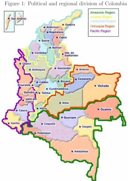
In order to examine these characteristics we divide the country in regions and subregions. For the regional division we follow traditional geography which divides the country in five areas: Amazonic, Orinoquia, Pacific, Car-ribean and Andean. On the other hand, to obtain the subregions we used the political division of the country which splits Colombia in 32 areas and the capital city, Bogot´a (see Figure 1).
To analyze the spatial concentration of banks we use the total number of branches per a 100,000 habitants as a measure. In first place, we calculate it for the regional scenario. As Table 1 shows, the variable reveals that the area with the highest branch concentration for 1996 was the Andean (5.13), followed in order by the Pacific (4.1), Caribbean (3.74) and Amazonic (1.98) regions. However, for 2005, the order changes and Orinoquia takes the first place, duplicating the value that it had in the first year of study (6.84). This table shows as well, the poor financial development of the Amazonic region, that had the lowest number of branches per habitant in the country through the whole period in study.
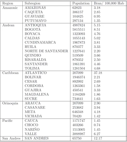
Further, we calculate the variable for each of the subregions for 1996 and 2005, the results are presented in Tables 2 and 3. On one hand, Table 2 shows that the departments with more branches per habitant for 1996 were Atl´antico (37.18), San Andr´es (12.17) and Bogot´a (8.51), while the least
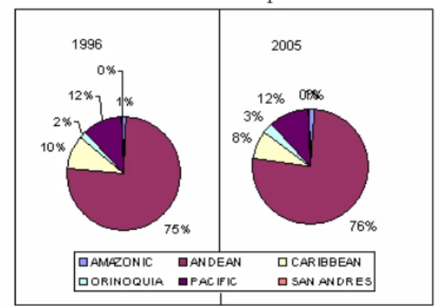
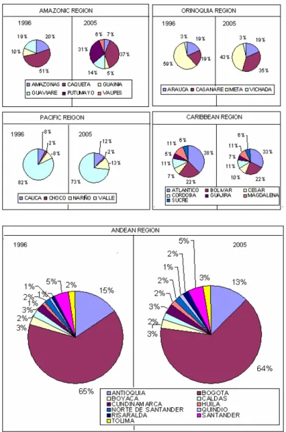
Figure 2: Distribution of deposits for each region
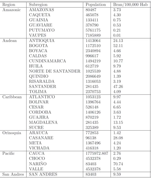
concentrated were Choc´o (0.74), Guaviare (0.95) and Putumayo (1.35). On the other hand, Table 3, reveals that in 2005 the subregions with the highest values were in order Nari˜no (70.74), Bogot´a (52.11) and Santander (47.26), whereas, the ones with the lower values were Choc´o (0.29), Putumayo (0.21) and Vaup´es (0.01).
When we check for the banks with the higher number of branches within the country, we found that the Banco de Bogot´a (343), Bancaf´e (297) and Banco Ganadero (163) had the biggest numbers for 1996. Nevertheless, for 2005, the banks that had more branches all around the country were the Banco Agrario (723), Bancolombia (379) and the Banco de Bogot´a (354).
On second place, to analyze the weigh of each area in the country deposit market we employ a simple ratio of the total deposits of the area and the total deposits of the country. As we did for the number of branches per 100,000 habitants we also calculated this variable for the regional and subregional dimensions.
For the regional division, as Figure 2 presents, in 1996 the Andean re-gion accounted for for 75 percent of the deposit market, while the Pacific, Caribbean and Orinoquia regions stand for the 12, 10 and 2 percent of the market, respectively. For 2005, the scenario is quite the same given that the Andean region represents 76 percent, and the Pacific, Caribbean and Orinoquia accounted for a 12, 8 and 3 percent of the market. It is worth mentioning that the Amazonic region reduced its market participation from 3 to almost zero percent between these two years.
More deeply, the weigh of each department inside each of the regions is presented in Figure 3. For the Amazonic region, we found that the most important subregions are Caqueta, which reduced its share in the market between 1996 and 2005, and Putumayo, area that gain importance through
Table 2: Spatial distribution for departments in 1996
Region Subregion Population Bran/ 100,000 Hab Amazonic AMAZONAS 62823 3.18 CAQUETA 386157 2.85 GUAVIARE 104825 0.95 PUTUMAYO 297134 1.35 Andean ANTIOQUIA 4987824 5.15 BOGOTA 5815511 8.51 BOYACA 1323093 4.76 CALDAS 1055143 5.02 CUNDINAMARCA 1967873 3.81 HUILA 870377 3.33 NORTE DE SANTANDER 1227641 2.20 QUINDIO 519509 3.66 RISARALDA 879352 2.50 SANTANDER 1861391 4.46 TOLIMA 1281504 4.68 Caribbean ATLANTICO 207099 37.18 BOLIVAR 1946374 2.21 CESAR 892992 2.69 CORDOBA 1263361 1.58 GUAJIRA 450541 3.33 MAGDALENA 1184269 1.86 SUCRE 734641 1.63 Orinoquia ARAUCA 207099 2.90 CASANARE 253682 3.94 META 646348 4.18 VICHADA 70420 1.42 Pacific CAUCA 1171747 1.45 CHOCO 403266 0.74 NARI ˜NO 1513005 1.45 VALLE 3888987 6.27
Table 3: Spatial distribution for departments in 2005
Region Subregion Population Bran/100,000 Hab Amazonic AMAZONAS 80487 3.73 CAQUETA 465078 4.30 GUAINIA 133411 0.75 GUAVIARE 378790 0.53 PUTUMAYO 5761175 0.21 VAUPES 7185889 0.01 Andean ANTIOQUIA 1413064 24.13 BOGOTA 1172510 52.11 BOYACA 2340894 4.66 CALDAS 996617 5.92 CUNDINAMARCA 1494219 10.77 HUILA 612719 9.79 NORTE DE SANTANDER 1025539 4.88 QUINDIO 2086649 1.39 RISARALDA 1316053 3.19 SANTANDER 281435 47.26 TOLIMA 2370753 4.09 Caribbean ATLANTICO 1053123 9.97 BOLIVAR 1396764 4.44 CESAR 526148 6.65 CORDOBA 1406126 3.63 GUAJIRA 870219 1.72 MAGDALENA 281435 13.15 SUCRE 325389 9.53 Orinoquia ARAUCA 772853 1.42 CASANARE 96138 28.08 META 1367496 4.24 VICHADA 416318 1.20 Pacific CAUCA 1775972.807 2.76 CHOCO 4532378 0.29 NARI ˜NO 83403 70.74 VALLE 4532378 5.58
Table 4: Colombian Banking: Sample descriptive statistics for 1996 and 2005
1996 2005
Average Median Average Median Deposits 445973323.4 313469448.5 3137285066 1943985681
wl 37549.06135 22274.36581 46918.11174 20275.22707
wk 2.666434695 2.647224659 3.806171451 3.514046784
rd 0.186013163 0.188642616 0.052052311 0.050732414 Branches 79.63636364 27 170 123
the period in study. On the Orinoquia region for 2005, the biggest markets were Meta and Casanare while for the Carribean region Atl´antico was the most important. Finally, in the Andean region the most relevant market in 2005 was Bogot´a accounting for 64 percent.
For a brief summary of the statistical analysis of the aggregated variables applied in the model estimation see Table 4.
5.4
Estimation
As pointed out the model was estimated in two stages, one concerning each period. In both periods, time-series and cross section data were pooled25. In the first period, we used aggregated data for the whole country, and for the second period, we made two estimations. In part A of the second period we divide the country in five regions and in part B the country was divided in 33 subregions, see Table 5.
For the first period we estimate the equation that specifies the first order condition for the deposit interest rate (4.4) and the demand equation (5.1) by full information maximum likelihood method, where the marginal cost functional form was given by equation 5.2.
Using the same method, for the second period we estimate as well the first order condition for the number of branches in each local market (4.9), and the demand equation (5.3) for each of the regions and subregions, where the functional form for the regional marginal cost was represented by equation 5.4.
5.5
Results
Tables 6, 7,8 and 9 present the results of the complete estimation of the two period model. For the first period (Table 6) we obtained parameters that are statistically significant and consistent with the microeconomic theory. For the deposit supply, the partial derivative with respect to the own interest rate is positive, while the partial derivative with respect to the weighted average of the rivals interest rate is negative. Additionally, the relation between the deposit supply and the general domestic product is positive, and the number of employees, that was used as a proxy of the firms’ size, reveals that larger firms face bigger deposit supply. On the other hand, for the marginal cost function the results are as well satisfactory showing positive signs for b1, b2 and b3.
For this estimation, the conjectural parameter γ rejected the existence of market power in the deposit market, given that the estimate was less than zero. This result is in line with the empirical research made for the Colombian deposit market in which Estrada (2005) and Salamanca (2005) have found evidence of a market structure more competitive than the Nash equilibrium for the deposit market26.
25This estimation follows the procedure applied in Canhoto (2004).
26In the international literature Bikker and Haaf (2000) found also evidence of
Table 5: Territory divisions taken for the estimation
PERIOD 1 PERIOD 2
PART A PART B Colombia Amazonic Amazonas
Guainia Guaviare Vaupes Caqueta Putumayo Orinoquia Arauca Casanare Vichada Meta Andean Antioquia Santander N. de Santander Boyaca Cundinamarca Huila Risaralda Quindio Bogota Tolima Caldas Pacific Choco Valle Cauca Nari˜no Caribbean Guajira Cesar Magdalena Atlantico Bolivar Sucre Cordoba
Table 6: Estimation results for the first period
Parameters Estimate St. Error T-statistic p-value
a0 3.91E+08 4.79E+08 0.817193 0.414 a1 1.62E+09 7.61E+08 2.13157 0.033 a2 -1.22E+10 1.03E+09 -11.9066 0.000 a3 55.8835 20.0602 2.78579 0.005 a4 478833 21222.9 22.5621 0.000 b0 -0.99722 0.0892 -11.1796 0.000 b1 7.83E-03 1.76E-03 4.43983 0.000 b2 0.016598 4.22E-03 3.93026 0.000 b3 0.037086 4.21E-03 8.80852 0.000 γ -2.6108 0.395549 -6.60044 0.000 The estimated equations were:
r∗ i = µ rs(1−p) +mp−dCi(Di) dDi ¶ −Diµ 1 (∂Di ∂rd i ) + ( ∂Di ∂rd Ri)(γ) ¶ (5.5) Di=a0+a1rid+a2rRid +a3gdp+a4empi+εi (5.6) where: dCi(Di) dDi =M C d i =b0+b1wli+b2wki+b3Di+²i (5.7) As it was pointed out the equations were estimated by full information maximum likelihood using TSP 4.5.
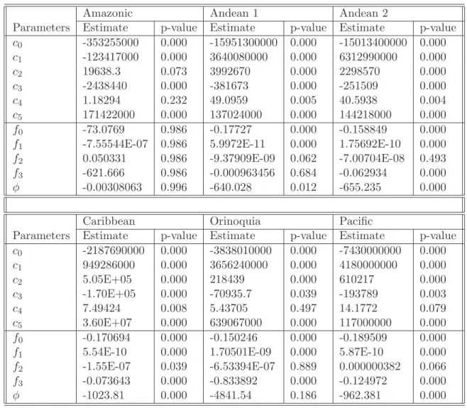
In this same way, the results for the estimation of the part A of the second period, in which the country was divided in five regions, are presented in Table 7. We made two estimations for the Andean region, Andean 1 includes the capital city of the country and Andean 2 does not includes it. For this division we found nonsignificant parameters for the Amazonas and the Orinoquia regions, which could be explained by the size of the markets and its poor development. For the other regions, most of the parameters were significant and showed the expected signs27. With respect to the conjectural parameters (φ), we found that all the regions appear to have competitive markets 28. More specifically, the Caribbean region appeared to have the lower conjectural parameters (φ = −1023.81), followed by the Pacific (φ =
−962.381) and Andean1 (φ =−640.028).
The results concerning the estimation of the second period in a more disaggregated approach are presented in Tables 8 and 9. For this phase, the parameters could not be estimated or were nonsignificant for Arauca, Casanare, Guain´ıa, Choc´o, Guaviare, Quind´ıo, Sucre, Tolima, Vaup´es, Meta, Huila y Putumayo. For the rest of the subregions the conjectural parameters were significant and signs were consistent with theory. In this estimation we found some areas that present evidence of market power. More specifi-cally, we found that Caquet´a (φ = 2569), Cauca (φ = 1848) and Norte de Santander(φ= 793) are the less competitive subregions of the country.
Summarizing, although we found evidence of a competitive national de-posit market, when we analyze the market in a more disaggregated approx-imation we found that there are some subregions that present evidence of market power. In particular, we found that Caquet´a, Cauca and Norte de Santander present collusive market structures in their deposit markets. In this context, within these regions regulation policies should be carefully ad-dressed to avoid bigger market structure problems, or even better, to improve competitive conditions.
Finally, this results prove that market structure is not properly analyzed in very big markets were the results are too general and may lead to wrong regulatory measures.
27There are some problems with the signs of some parameters in the marginal costs.
However, problems that concern incoherence of the coefficients of the marginal costs are common in the literature of conjectural parameters.
Table 7: Estimation results for the second period. Part A
Amazonic Andean 1 Andean 2
Parameters Estimate p-value Estimate p-value Estimate p-value
c0 -353255000 0.000 -15951300000 0.000 -15013400000 0.000 c1 -123417000 0.000 3640080000 0.000 6312990000 0.000 c2 19638.3 0.073 3992670 0.000 2298570 0.000 c3 -2438440 0.000 -381673 0.000 -251509 0.000 c4 1.18294 0.232 49.0959 0.005 40.5938 0.004 c5 171422000 0.000 137024000 0.000 144218000 0.000 f0 -73.0769 0.986 -0.17727 0.000 -0.158849 0.000
f1 -7.55544E-07 0.986 5.9972E-11 0.000 1.75692E-10 0.000
f2 0.050331 0.986 -9.37909E-09 0.062 -7.00704E-08 0.493
f3 -621.666 0.986 -0.000963456 0.684 -0.062934 0.000
φ -0.00308063 0.996 -640.028 0.012 -655.235 0.000 Caribbean Orinoquia Pacific
Parameters Estimate p-value Estimate p-value Estimate p-value
c0 -2187690000 0.000 -3838010000 0.000 -7430000000 0.000 c1 949286000 0.000 3656240000 0.000 4180000000 0.000 c2 5.05E+05 0.000 218439 0.000 610217 0.000 c3 -1.70E+05 0.000 -70935.7 0.039 -193789 0.003 c4 7.49424 0.008 5.43705 0.497 14.1772 0.079 c5 3.60E+07 0.000 639067000 0.000 117000000 0.000 f0 -0.170694 0.000 -0.150246 0.000 -0.189509 0.000
f1 5.54E-10 0.000 1.70501E-09 0.000 5.87E-10 0.000
f2 -1.55E-07 0.039 -6.53394E-07 0.889 0.000000382 0.066
f3 -0.073643 0.000 -0.833892 0.000 -0.124972 0.000
φ -1023.81 0.000 -4841.54 0.186 -962.381 0.000 The estimated equations were:
µ rs(1−p) +mp−rd∗ i − dCik(Dik) dDik ¶µ ∂Dik ∂nik + ∂Dik ∂n−ik φ ¶ =dCik(nik) dnik (5.8) Dik=c0+c1rid∗+c2nik+c3n−ik+c4gdp+c5( popk km2k ) +µi (5.9) dCi(Di) dDi =M C d ik=f0+f1wlik+f2wkik+f3Dik+νi (5.10) As it was pointed out the equations were estimated by full information maximum likelihood using TSP 4.5.
Table 8: Estimation results for the second period, part B
Department c0 c1 c2 c3 c4 c5
Amazonas -2.40E+08 3.01E+08 NE 881994 0.149872 **3.3E+08 Antioquia *-1.8E+10 *1.2E+10 *5758330 *-241150 **33.2666 *1.9E+08 Arauca -9.81E+09 1.50E+10 1.60E+06 -1.98E+06 3.18E+01 7.41E+08 Atlantico *-2.6E+08 *1.9E+08 *5674000 *-329296 0.932553 *3629370 Bogota *-7.3E+09 *2.8E+09 *12257800 *-700903 **24.3169 *1899800 Bolivar *-5.8E+08 *3.6E+08 *1526000 -47051.3 *2.16744 *6187480 Boyaca *-3.1E+09 *7.0E+08 *2121770 *-220286 2.8152 *51362900 Caldas *-9.3E+08 *3.8E+08 *5187030 -46034.3 *1.94209 *6071100 Caqueta *-1.1E+08 *3.7E+07 *513298 113611 0.310923 *23278400 Casanare *-1.6E+13 *1.9E+13 340209 -85781 63355.5 1.93E+12 Cauca *-5.8E+08 *3.3E+08 *2155520 *138265 2.01306 *12148100 Cesar *-3.1E+09 *1.2E+08 *2359800 *-300152 *0.945732 *7243140 Choco -1.13E+10 2.83E+09 604323 906076 5.70251 1.25E+09 Cordoba *-4.2E+09 *2.1E+09 *1833920 *-280249 5.746 *73730600 Cundinamarca *-2.8E+09 *2.1E+09 *2032240 *-270290 *7.82205 *27773700 Guainia 4.51E+09 -1.98E+10 NE -5.55E+06 -44.3583 -5.26E+09 Guajira *-1.3E+09 *8.4E+08 *3034290 *-1471290 2.5893 *52676800 Guaviare -2.79E+08 **3.6E+08 NE 1.08E+07 1.86025 9.78E+07 Huila *-5.5E+08 *1.5E+08 *909407 **-77094.7 *1.39148 *11355100 Magdalena *-2.9E+08 *1.2E+08 *2025630 *-155761 *1.01577 *4957050 Meta *-1.6E+08 -7.09E+07 64280.8 1381.43 -1.46073 *28210500 N. de Santander *-3.7E+08 *2.1E+08 *2543610 226277 1.02662 *5426890 Nari˜no -3.57E+09 2.75E+09 *596128 -22548.4 7.65294 6.32E+07 Putumayo *-1.6E+08 -1.42E+08 *-2697530 -718168 1.33806 *14268200 Quindio -3.03E+10 2.80E+10 170835 -3.81E+04 62.862 8.41E+07 Risaralda *-3.7E+08 *1.4E+08 *5797340 *-226826 *0.82286 *1528390 Santander *-1.4E+10 *1.2E+10 *2207590 *-881473 *29.2664 *271441000 Sucre *4.3E+13 -1.15E+14 68507.1 -2.04E-05 *-1368370 -638617 Tolima -5.71E+11 8.66E+10 *1207020 -194246 253.833 1.01E+10 Valle *-4.8E+09 *2.6E+09 *5288270 *-307278 *10.0526 *23266300 Vaupes 3.06E+09 -1.48E+10 NE NE -27.8194 -3.64E+09 Vichada *-2.5+E08 *3.7E+08 -2.40E+06 5.98E+06 -1.04607 *305058000 The estimated equations are the same of Table 3 and they were estimated by full
informa-tion maximum likelihood using TSP 4.5. The symbols ∗ and ∗∗ stand for significance of
5 and10percent, respectively. On the other hand the NE letters mean that the parameter couldn’t be estimated.
Table 9: Estimation results for the second period, part B
Department f0 f1 f2 f3 ψ
Amazonas **4585150 5234.24 1.20E+08 *-0.854899 NE
Antioquia *-0.161108 *2.01295E-06 *-0.604809 *1.00212E-09 **-1253.02 Arauca *-0.138958 -1.95E-05 *-1.16669 *3.57453E-09 -97.2559 Atlantico *-0.157279 *-0.400559E-07 *-0.079261 *1.07066E-09 *-460.717 Bogota *-0.177302 **-9.22785E-09 -1.04E-03 *9.5709E-11 *-399.093 Bolivar *-0.21762 -4.36E-08 *-0.109921 *3.81219E-19 *-3683.01 Boyaca *-0.134089 *-1.33349E-05 *-0.410156 *1.47714E-09 *-928.902 Caldas *-0.128577 1.52E-07 *1.52078E-07 *1.02645E-09 *-2649.84 Caqueta *-0.187033 *-0.0000563726 6.68E-02 *8.17598E-09 *2569.62 Casanare -0.269125 -1.91E-04 -5.94347 1.18E-08 -8527.9 Cauca *-0.152278 *-0.0000126883 *-0.498274 *2.83899E-09 *1848.01 Cesar *-0.150596 *-0.0000164335 *-0.716753 *3.54418E-09 *-822.75 Choco *-0.188187 -8.30E-06 -1.52325 *7.9E-09 376.096 Cordoba *-0.170218 -8.82E-06 *-3.65047 *7.02E-09 *-872.336 Cundinamarca *-0.157036 *-0.00000245623 *-0.328134 *1.5E-09 *-993.436 Guainia -3.15E+08 -275714 -1.28E+10 33.3261 NE Guajira *-0.127416 *-0.0000873574 *-2.56471 *4.9E-09 *-194.757 Guaviare 7.77E+06 4181.19 4.49E+07 *-0.639803 NE Huila *-0.154926 *-0.0000190607 *-0.24298 *2.9E-09 -6113.07 Magdalena *-0.184234 *-0.00000710101 -0.033951 *4.7E-09 **-2401.99 Meta -4.04133 2.84E-04 -36.8656 -8.55E-08 189.064 N. de Santander *-0.174544 *-0.00000303999 *-0.508143 *2.82197E-09 *793.597 Nari˜no *-0.170376 *0.0000026164 *-0.747875 *3.01824E-09 *-8932.56 Putumayo -0.349578 -3.09E-03 42.1371 1.53E-07 -3.00581 Quindio *-0.085774 *0.0000469452 *-3.50385 *2.29446E-09 *-2053.27 Risaralda *-0.146353 -1.18E-07 -0.021445 *9.76345E-10 *-481.207 Santander *-0.178559 *0.00000602752 *-0.763949 *2.03916E-09 *-238.119 Sucre -1.36E+09 -733.949 -2.88E+07 77.5182 -8.46E+13 Tolima 1.79731 4.65E-05 -17.4433 1.69E-08 -12009 Valle *-0.181632 *0.000000328566 *-0.106415 *6.48948E-10 *-578.46 Vaupes -2.95E+08 65414.1 -9.73E+09 22.0264 NE Vichada -0.122635 -5.10E-04 -14.8492 1.53E-08 -32.1951 The estimated equations are the same of Table 3 and they were estimated by full
informa-tion maximum likelihood using TSP 4.5. The symbols ∗ and ∗∗ stand for significance of
5 and10percent, respectively. On the other hand the NE letters mean that the parameter couldn’t be estimated.
6
Concluding comments
In this paper we develop a multimarket spatial competition oligopoly model in which banks compete with price (interest rates) and non price (branches) variables in the deposit market. In this context, each bank chooses the opti-mal interest rate that it will fix for all the country in a first period, and in a second period given that interest rate, each bank chooses the optimal number of branches that it should open in each region of the country to maximize its profit function. For the second period, we take two approximations. In part A we divide the country in 5 regions and then in the other approach we divide it in 33 subregions (part B).
The purpose of the proposed model was to test for competitive conditions in a more disaggregated approach, in order to state if the conclusions obtained by studying each region and subregion of the country are different from the ones obtained by the analysis of the whole national markets.
The theoretical model was applied to quarterly data that covers the 1996-2005 period. The data was pooled and the estimation was made by full information maximum likelihood for each period.
Our empirical results for the first period reveal, that the deposit market in the whole country is characterized by a competitive market structure. In this same way the results for the part A of the second period, show that deposit market of the Caribbean, Pacific and Andean are as well competitive markets. However in the estimation of part B of the second period, we found that there are some local areas that present evidence of market power. In particular, we identify three critical markets: Caquet´a, Cauca and N. de Santander.
In this way, we suggest that regulation policies should be carefully ad-dressed in these three critical markets to avoid bigger competition problems. Additionally, from this results we were able to prove that the market struc-ture is not properly measure in big markets were the results are too general and may lead to wrong regulatory measures.
Finally we must say, that this work opens new questions for the research area. For instance, new studies should try to explain why banks tend to agglomerate in some regions leaving aside other important areas.
References
Angelini, P., and Cetorelli, N. (2000). Bank competition and regulatory re-form: the case of the Italian banking industry. Federal Reserve Bank of Chicago.
Barajas A., Salazar, N. and Steiner, R. (1999). Interest spreads in banking in Colombia: 1974-1996.Staff Papers, International Monetary Fund.. Vol. 46.
Barajas, Salazar and Steiner (2000). The impact of liberalization and for-eign investment in Colombia’s financial sector. Journal of Development Economics. Vol.63, pp. 157-196.
Barros, P. (1997). Multimarket competition in banking, with an example from the Portuguese marketInternational Journal of Industrial Organiza-tion. Vol.17, pp. 335-352.
Berg S. A., and Kim M., (1994). Oligopolistic interdependence and the struc-ture of production in banking: An empirical evaluation.Journal of Money, Credit and Banking. Vol.26 pp. 309-322.
Berg S. A., and Kim M., (1996). Banks as multioutput oligopolies: An empir-ical evaluation of the retail and corporate banking markets.Federal reserve bank of Chicago.
Bikker J. A., and Haaf, K.(2000). Competition, concentration and their rela-tionship: An empirical analysis of the banking industry.Economic Letters. Vol.10, pp. 87-92.
Bowley, A. (1924). The mathematical groundwork of economics.Oxford Uni-versity Press.
Bresnahan, T. (1982). The oligopoly solution concept identified. Economic Letters Vol.10, pp. 87-92.
Cabral, L.(1995).Conjectural variations as a reduced form.Economic Letters. Vol. 49, pp. 397-402.
Canhoto, A.(2004). Portuguese banking: A structural model of competition in the deposti market. Review of financial economics. Vol. 13, pp. 41-63. Canoy, M., Dijik, M., Lemmen, J., Mooji, D., R., and Weigand, J.(2001).
Competition and stability in banking. Netherlands Bureau for Economic Policy Analysis.
Chiappori, P. A., D. Perez-Castrillo, and Verdier D., (1993). Spatial competi-tion in the banking system: Localizacompeti-tion, cross subsidies and the regulacompeti-tion of deposit rates. European Economic Review. Vol. 39, pp. 889-918.
Estrada, D.(2005). Efectos de las fusiones sobre el sector financiero colom-biano. Banco de la Rep´ublica de Colombia.
Frazer and Zakoohi (1998). Geographical deregulation in the U.S. banking markets.Financial Review. Vol.33, pp.85.
Freixas, X., and Rochet, J., (1997). Microeconomics of banking.Cambridge: MIT Press.
Frisch, R. (1951). Annual survey of economic theory International Economic Papers. Vol. 1, pp. 23-36.
Gelos G., and Roldos J.(2002). Consolidation and market structure in emerg-ing markets bankemerg-ing systems.IMF. No.186
Gilbert A.(1984). Bank market structure and competition.Journal of Money, Credit and Banking. Vol. 16, pp. 205-218
Hannan T., And Liang, (1993). Inferring market power from time series data.International Journal of Industrial Organization. Vol. 11,No.4.
Iwata, G.(1974). Measurement of conjectural variations in
olipoly.Econometrica. Vol. 42, No. 5, pp.947-966.
Kim, M., and Vale, M.(2001). Non-price strategic behavior: the case of bank branches.International Journal of Industrial Organization. Vol. 19, pp. 1583-1602.
Kim, M., Vivas, A. L., and Morales A.(2003). Multistrategic spatial compe-tition with application to banking. University of Malaga.
Lau, L. (1982). On identifyng the degree of competitiveness from industry price and industrial data.Economic Letters. Vol.10, pp. 93-99.
Levy, E., and Micco, A.(2003). Concentration and foregin penetration in Latin American banking sectors: Impact on competition and risk.Escuela de negocios. Universidad Torcuatto Di Tella.
Mora, H. (2004). Eficiencia de los sistemas bancarios de los pa´ıses miembros
Neven, D., and Roller, L.(1999). An aggregate structural model of competi-tion in the European banking industry.International Journal of Industrial Organization. Vol.17, pp. 1059-1074.
Panzar, J., C., and Rosee, J., N.(1987). Testing for monopoly equilib-rium.Journal of Industrial Economics. Vol.35, pp. 443-456.
Reyes, C.(2004). El poder de mercado de la banca privada colombiana. Mag-ister Thesys, Universidad de los Andes.
Salop, S.(1979). Monopolistic competition with outside goods.The Bell Jour-nal of Economics. Vol. 10, No. 1, pp. 141-156.
Schmalensee, R. (1989). Good Regulatory Regimes. Rand Journal of
Eco-nomics. Vol. 20, No. 3, pp. 417-436.
Salamanca, D.,(2005). Competencia en los mercados de credito y depositos en Colombia: aplicacion de un modelo de oligopolio fijador de precios.
Universidad de los Andes.
Shaffer, S.(1989). Competition in the US banking industryEconomic Letters. Vol. 29, pp.321.
Shaffer, S.(1993). A test of competition in Canadian banking. Journal of Money, Credit and Banking. Vol. 25, pp.49-61.
Swank, J.(1995). Oligopoly in loan and deposit markets: An econometric application to the Netherlans. De Economist.Vol. 143, pp.353-366. Suonemin, N.(1994). Measuring competition in banking: A two product
model.Scandinavian Journal of Economics. Vol. 96, pp.95-110.
Toolsema L.,(2002). Competition in the Dutch consumer credit mar-ket.Journal of Banking and Finance. Vol. 26.
Uchida, H., y Tsutsui, Y., (2005). Has competition in the Japanese banking sector improved?.Journal of Banking and Finance. Vol. 29.
Vesala J., (1995). Testing competition in banking: behavioral evidence from Finland. Bank of Finland Studies.