Buyback of Colombian Sovereign Debt

(1)

Buyback of Colombian Sovereign Debt

Peter Rowland Banco de la República*

Abstract

At a request from the Ministry of Finance, Banco de la República last year carried out an investigation into the feasibility to use parts of the foreign reserves to buy back some of Colombia’s outstanding sovereign U.S.-dollar debt. This project resulted in two thorough technical reports. This paper aims to complement these reports by a general discussion on the subject. Even if many economists will find the discussion and the empirical results interesting, the main target group of the paper is professionals and policy makers without a background in Economics or Finance. The paper discusses emerging market debt in general, the Colombian debt in particular, and the current level of the Colombian foreign reserves. It, thereafter, continues by discussing buyback of sovereign debt, and what a country could gain or lose from such a buyback and why. The paper also includes a cross-country empirical analysis of the relationship between the sovereign spread of the outstanding debt of a country and its foreign reserve levels.

*_{The opinions expressed here are those of the author and not necessarily of the Banco de la República, the}

Colombian Central Bank, nor of its Board of Directors. I express my thanks to Javier Gómez, and Franz Hamann for helpful comments and suggestions. Any remaining errors are my own.

(2)

1 Introduction

Last year, the Ministry of Finance asked Banco de la República to carry out a technical investigation into the proposal by the President of the Republic, to “invest any possible surpluses of the international reserves, which are fiscally expensive, to obtain a better economic and social use of such funds”. The idea, which had originally been raised by some members of Congress in 2002, was to invest any excess reserves in Colombian sovereign debt, i.e. to buy back such debt. The rationale was that while Colombia pays a relatively high rate of interest on its sovereign debt, the return on the foreign reserves is significantly lower.

The Bank carried out a thorough investigation into this subject, which was documented in two reports, Análisis del nivel adecuado de reservas internacionales,1 and El nivel de las reservas internacionales y su manejo reciente.2 Both these reports are by their nature very technical and might be difficult to follow by people without a background in Finance or Economics. This current paper aims to complement these two reports by discussing the issue of sovereign debt buyback in a rather un-technical fashion. The paper is aimed at a target group including professionals and policy makers without a background in Economics and Finance, as well as people working in those areas.

Debt buyback is, furthermore, not a subject related only to Colombia, but something that has been considered by many emerging market economies. The paper aims to give the reader a good introduction to the subject, and, in addition, it presents some interesting empirical results.

The paper is organised as follows: Chapter 2 discusses emerging market debt in general as well as valuation of emerging market bonds, to build an understanding of the dynamics in this part of the financial markets. Chapter 3 continues by discussing the Colombian sovereign debt in particular. The Colombian foreign reserves and whether these can be

1_{Banco de la República (2003).} 2_{Banco de la República (2004).}

(4)

regarded as excessive, is analysed in chapter 4. Chapter 5 looks at the question whether swapping part of the low-risk low-yielding securities of the foreign reserves into Colombian sovereign debt would be a good trade. Chapter 6 presents a cross-country empirical investigation into the relationship between the levels of foreign reserves and the sovereign spread of emerging market economies. A discussion of the Bolivian debt buyback of 1988 is also included in this chapter. And finally, chapter 7 concludes the paper.

(5)

2 Emerging Market Debt

This chapter aims to give the reader an introduction to traded emerging market debt, and especially how such debt is priced. In the next chapter we will discuss the Colombian debt in particular. Section 2.1 discusses emerging market sovereign debt and the recent spread history of such debt. In section 2.2, valuation of emerging market issues is analysed.

2.1 Emerging Market Sovereign Debt

Emerging market debt was hardly traded at all before the 1990s.3 While banks held 97 percent of all emerging market debt at the end of the 1980s, their share had fallen to less than two thirds by the mid-1990s.4 The change was initiated by Mexico launching its Aztec bond in March 1988.5 This was followed by the Brady Plan in 1989, which was a programme initiated by the U.S. government, to allow emerging markets to issue bonds in exchange for rescheduled bank loans. The so-called Brady bonds were partly collateralised by U.S. Treasuries. The first country to reach a Brady agreement was Mexico, and Mexico has since then been used as a benchmark for pricing emerging market debt. A total of 17 countries have taken advantage of the programme, with a cumulative face value of USD 170 billion of Brady bonds issued.6

The Brady bonds transformed the market from sovereign debt ownership concentrated in the hands of a few creditor banks and dealers to ownership distributed more widely through an actively traded and liquid Brady bond market. This also opened the doors for

3_{Latin America had large traded debt issues in the 1920s. However, with the Great Depression and}

following debt defaults, Latin American traded debt almost completely disappeared. See, for example, Eichengreen and Portes (1986).

4_{Eichengreen and Mody (1998), p. 7.}

5_{This was a 20-year USD 2.6 billion issue in exchange for rescheduled bank loans. Its principal was fully}

collateralised with special purpose bonds issued by the U.S. Treasury.

(6)

emerging market eurobond issues. Emerging market bonds are today a common component of the portfolios of institutional fixed income investors.

Colombia has in modern times not defaulted on its sovereign debt, and has, therefore, never issued any Brady bonds.7 It has, nevertheless, a number of outstanding eurobond issues.

Emerging market bonds are normally priced as a spread8 over the U.S. Treasuries curve.9 We will throughout this paper use the EMBI10 Global composites, as calculated by JP Morgan, to represent the sovereign spread over U.S. Treasuries.11 The EMBI Global composites are weighted averages of the spreads of U.S. dollar-denominated individual bonds issued by a particular emerging market country.12 Figure 2.1 shows the development of JP Morgan’s EMBI Global spread composite from 1998 up until present.

7_{Colombia did, indeed, default on its sovereign debt in the 1930s together with most other Latin American}

sovereign issuers, but has not defaulted since then.

8_{The spread of a U.S. dollar denominated bond is typically defined as the difference in yield between that}

bond and a benchmark U.S. Treasury bond of the same maturity and is normally expressed in basis points, where one basis point is 1/100 or a percent.

9_{Some authors have, indeed, questioned this practice, arguing that emerging market bonds should be priced}

in terms of absolute yield instead rather than in terms of spread to Treasuries. See Vine (2001) for a discussion.

10_{Emerging Market Bond Index.}

11_{Some studies have selected a benchmark bond for each country studied and used its spread; others have}

looked at the spreads of several individual bonds. Since we are in this study looking at the spread related to the risk of a sovereign issuer rather than the spreads of individual bonds, the EMBI Global suits our purpose better than using individual bonds. The EMBI Global composite, furthermore, controls for floating coupons, principal collateral, rolling interest guarantees, and other unusual features of the bonds, and it is computed for all the main emerging market sovereign issuers, making comparisons easy.

12_{The EMBI Global composite, which was introduced in August 1999, is the most comprehensive}

emerging markets debt benchmark. It followed the EMBI and EMBI Plus, where the former is a pure Brady bond composite, and the latter includes eurobonds as well. The EMBI Global include, in addition to Brady bonds and eurobonds, U.S. dollar-denominated traded loans and local market debt instruments issued by sovereign and quasi-sovereign entities. Only issuers from low- and middle-income countries are included in the index, and only issues with a time to maturity of 2.5 years or more and a current face value outstanding of at least USD 500 million. The index is calculated as an average weighted by the current market capitalisation of the individual issues. See JP Morgan (1999) for a further discussion on how the

(7)

Figure 2.1: EMBI Global Spreads 1998 – 2004 (basis points) Source: Rowland (2004b). 0 200 400 600 800 1000 1200 1400 1600 1800 1998 1999 2000 2001 2002 2003 2004 Russia devalues Ruble and halts

foreign debt payments Brazil Real devaluation Ecuador misses scheduled Brady payment Russia defaults on restructured Vnesh loans September 11 attacks on the U.S. Argentina devalues Peso and defaults

on foreign debt Lula elected president in Brazil Argentina defaults on World Bank debt Irak war begins USD 30 bn IMF rescue package for Brazil announced

(8)

2.2 Valuation of Emerging Market Issues

When analysing emerging market bonds, it is completely crucial to understand how these bonds are priced by investors, as well as the fundamental differences between sovereign and corporate debt.13 Corporate debt, particularly high yield debt,14 can be priced using option theory. The principal for such a valuation procedure is explained in box 2.1.

Box 2.1. Valuing corporate debt using option theory

We let D represent the market value of the corporation’s debt, which is the promise to pay the face value F of the debt in t years. We, furthermore define S as the market value of the firm’s common stock and A as the current market value of its assets. The Modigliani-Miller theorem (Modigliani and Miller (1958) in their seminal paper affirmed that the value of a firm should be independent of its capital structure) states that,

A = D + S (2.1)

Given this structure, the firm’s common stock can, indeed, be interpreted as a call option on its assets with an exercise price of F and an expiration time t. When the debt matures, the stockholders have the choice either to pay the face value F of the bond to the creditors, which would represent to exercise the call option, or to default on the debt and let the creditors take control of the assets of the firm, which would represent not exercising the option. Option pricing theory (normally the Black-Scholes option pricing model, which is derived and discussed in, for example, Hull (2002)) can now be used to value the common stock S of the company, and the value of the debt can be calculated using equation (2.1).

(9)

The valuation of sovereign debt is not as straight forward, which has to do with the difference in default procedures involving corporate and sovereign debt respectively. A firm normally defaults on its debt when the value of its common stock falls to zero, and the firm, therefore, turns insolvent. It goes into bankruptcy proceedings whereby control of its assets is transferred to its creditors. If the firm is liquidated, the assets are sold and the proceedings divided by the creditors according to well-defined rules.

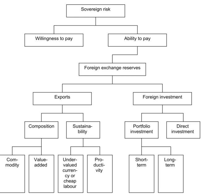
The default of a sovereign debtor is much more complicated.15 Sovereign default risk is related to both the issuer’s ability to pay and its willingness to pay, as illustrated by figure 2.2. A sovereign does, furthermore, not have a well-defined asset base, and the creditors normally have very limited possibility to take control of any assets of the sovereign.16 When a sovereign defaults, its debt is normally restructured through lengthy negotiations with its creditors, and the outcome of any such negotiations can be hard to predict. No clear framework for sovereign default proceedings is in place, and a sovereign default is normally a very complicated affair.17

15_{The complexity of strategic issues involved in lending to a sovereign nation has been discussed in a rich}

theoretical literature started by Eaton and Gersovitz (1981). See also Eaton, Gersovitz and Stiglitz (1986), as well as, for a less formalised analysis, Eaton and Taylor (1986).

16_{For this reason, option-pricing models are not very useful in valuing sovereign debt. Claessens and van}

Wijnbergen (1993), nevertheless, use option theory to price the bonds of the Mexican Brady deal. The value of the asset base A for a sovereign is not well defined, and Claessens and van Wijnbergen assume a stochastic behaviour for the value correspondent to A. They assume a Brownian motion even if there is no clear evidence for such behaviour of the underlying stochastic element. The model does, furthermore, neither take into account the behaviour of fundamental economic variables, nor any contagion effects. In spite of this, the paper offers some interesting theoretical insights.

17_{The IMF, among others, has been promoting the definition of a framework of clear sovereign}

restructuring proceedings, but so far no such framework has been agreed upon. Even if such a framework would be implemented, it would not cover bonds currently outstanding, only new issues. See Krueger (2002) for a suggestion and discussion of such a framework.

(10)

Figure 2.2: Analysis of sovereign risk

Source: Vine (2001), p. 525.

Sovereign risk

Willingness to pay Ability to pay

Foreign exchange reserves

Exports Foreign investment

Composition

Sustaina-bility investment Portfolio investment Direct

Com-modity Value-added Under-valued curren-cy or cheap labour

Short-term Long-term

Pro- ducti-vity

(11)

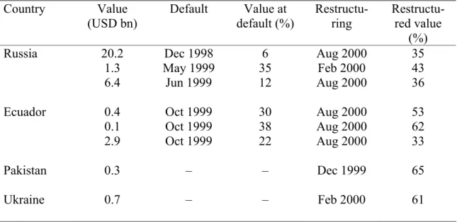
Table 2.1: Selected recent sovereign-debt restructurings Country Value

(USD bn) Default Value default (%) at Restructu-ring Restructu-red value (%)

Russia 20.2 Dec 1998 6 Aug 2000 35

1.3 May 1999 35 Feb 2000 43

6.4 Jun 1999 12 Aug 2000 36

Ecuador 0.4 Oct 1999 30 Aug 2000 53

0.1 Oct 1999 38 Aug 2000 62

2.9 Oct 1999 22 Aug 2000 33

Pakistan 0.3 – – Dec 1999 65

Ukraine 0.7 – – Feb 2000 61

Note: Value at default represents the market value as a percentage of the face value at time of default. Restructured value represents the market value of new bonds as a percentage of original face value.

Source: Economist (2004).

Table 2.1 shows the restructured value of sovereign debt after a number of recent debt restructurings. It is apparent that the restructured value of the debt has been in the range of 35 to 65 percent of the original face value of the debt. In comparison, Argentina, which in December 2001 defaulted of over USD 100 billion, the largest such default ever, are trying to reach an agreement with creditors to accept new bonds worth only 20 to 25 percent of the originals, which would be considerably less than in other recent restructurings.18

Even if outright sovereign defaults driven strictly by political considerations are very rare,19 the perceived willingness of a sovereign government to pay plays an important role in assessing the default risk and, thereby, also the value of sovereign debt. A

18_{See, for example, Economist (2004), for a discussion.}

19_{In this century, there have been only four major cases of sovereign default driven strictly by politics or}

ideology. In 1917, the Bolshevik government of Russia repudiated foreign obligations of the tsar. In 1934, Adolf Hitler repudiated much of Germany’s obligations under the Versailles Treaty. Japan followed a similar path in 1941, as did communist China in 1949. Vine (2001).

(12)

sovereign default is largely a political decision. In relation to the Russian default of 1998, Deutche Bank wrote: “We continue to maintain that a default depends far more on Russia’s willingness to pay versus its ability to pay its debt”.20 When a sovereign defaults, the government has normally traded off the cost of servicing the current debt against the costs of repudiation, of having assets abroad seized and of having international trade impeded.21 These costs are generally not evaluated in strict economic terms, but rather in political terms relating to the governments popularity, its chances to continue to stay in power, as well as other personal incentives of individual politicians. A sovereign, furthermore, rarely makes an outright default, but instead forces a restructuring or renegotiation of its debt, and the same debt may, indeed, be repeatedly restructured.22 The government generally also trades off the costs of defaulting on internal versus external debt. The government’s willingness to pay is, furthermore, in general very difficult to estimate.

The sovereign’s ability to pay is more predictable. Figure 2.2 earlier shows the principle for the analysis of the ability to pay as suggested by Vine (2001).23 The foreign exchange reserves are the ultimate foreign currency funds with which the foreign debt is serviced. A country that receives a large part of its foreign exchange reserves through foreign investment is highly dependent on capital inflows and has only a limited ability to de-leverage. Prices on debt of countries with this characteristic tend experience high volatility. If a large part of foreign investment comes as portfolio investment, which tend to be short-term, this also increases the volatility. Direct foreign investment, on the other hand, tends to be longer-term, and also has the added benefit of improving the productivity of the country’s private sector.

The analysis of exports can provide perhaps the most meaningful insight of the country’s ability to pay and its long-term outlook. Exports are a key source for building foreign exchange reserves, and export revenues can provide an opportunity for a country to

20_{Deutche Bank Research (1998), p. 3.}

21_{See Bulow and Rogoff (1989a), Eaton and Gersovitz (1981), and Gibson and Sundaresan (1999).} 22_{See Bulow and Rogoff (1989b)}

(13)

leverage. A country that receives a large part of its foreign exchange reserves through exports is generally a more stable credit than a country that relies heavily on capital inflows. Analysis of the composition and sustainability of exports is, therefore, important. The composition of exports addresses whether a country exports value-added goods or commodities, where the latter generally are much more exposed to price fluctuations adding to the volatility of the credit profile. The sustainability addresses whether a country exports because of high productivity or because of cheap labour or an undervalued currency. Generally, countries that have invested in productivity should outperform in terms of exports.

Another important factor when evaluating a country’s creditworthiness is the composition of its imports, specifically the proportions of consumption, intermediate and capital goods. The credit condition of a country that imports primarily capital goods financed with long-term money, such as for example the Asian tigers,24 would generally be stronger than that of a country that imports primarily consumption goods financed with short-term money, such as for example Mexico in 1994.

Other indicators analysed by investors when valuing debt includes inflation, the fiscal deficit and the gross domestic product. The rate of inflation is an indicator of the government’s discipline as well as its control over fiscal and monetary policy.25 A large fiscal deficit is problematic since it needs to be financed either through domestic or foreign borrowing. If the gross domestic product is contracting, this normally leads to a fall in government revenues, further aggravating the fiscal deficit. The government might try to increase revenues through tax increases, which would lead to further economic hardship.

In addition, there are many other indicators that influence sovereign creditworthiness. Such indicators include political and social stability in the country, unemployment, law and order, cooperation between central and provincial governments as well as between

24_{Hong-Kong, Singapore, South Korea and Taiwan.}

(14)

the different branches of the government, distribution of wealth, and respect for foreign investors and for international law. Another factor that directly influences the perceived credit risk is the country’s history of honouring debt obligations.26

The ability of investors to discriminate among emerging market sovereigns and to price risk appropriately has been controversial, to say the least. Some observers emphasise the cost involved in acquiring and processing the information relevant to assess a borrower’s creditworthiness.27 Investors, therefore, price debt on the basis of incomplete information about the borrowers’ economic and financial circumstances. This practice generates herding and market volatility.28

We can, nevertheless, conclude that the foreign exchange reserves of a country are completely crucial when analysing its foreign debt and when assessing the default risk of this debt.

26_{See, for example, Hajivassiliou (1989), and Özler (1993) for a discussion on the past history of}

repayments.

(15)

3 The Colombian Debt

After discussing emerging market debt in general, we will now analyse the Colombian sovereign debt. Section 3.1 introduces the Colombian debt, and compares a number of Colombian debt indicators with some other emerging market economies. Section 3.2 discusses the resent development of the Colombian spread and credit ratings. The section also includes a comparison of Colombia and other emerging market economies with similar credit ratings.

3.1 The Colombian Sovereign Debt

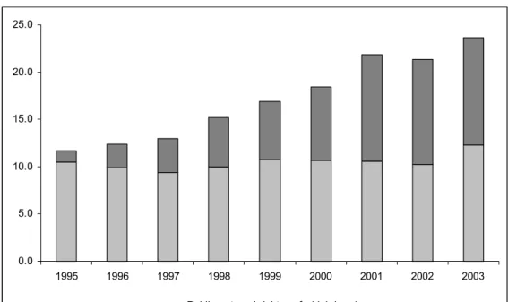
In line with many other emerging markets, Colombian sovereign bond issues surged during the 1990s. By the end of 2003, Colombia had an outstanding public external debt29 of USD 23.6 billion.30 Of this some USD 11.3 billion was bonds, a figure that increased rapidly during the 1990s, both in absolute terms an in relation to total public external debt, as illustrated by figure 3.1.

Colombia borrowed heavily during the second half of the 1990s, both internally and externally, to finance increasing fiscal deficits. These were further fuelled by the economic crisis of 1999, which was the first time in over 50 years that the country went through a recession.31 This lead to a rapidly increasing public debt.

29_{Debt denominated in other currencies than the Colombian peso.}

30_{This excludes the external debt of the public financial sector, which totals some USD 0.7 billion.}

31_{A recession is here defined as two consecutive quarters of negative economic growth. In 1999, real GDP}

contracted with as much as 4.2 percent, which is a very severe recession, indeed. Many observers would classify this as a depression.

(16)

Figure 3.1: Colombian external public debt, 1995 – 2003 (USD billion)

Source: Banco de la República

Figure 3.2: General government debt to GDP, 1997 – 2003 (%)

Source: Moody’s Investor Service.

0.0 5.0 10.0 15.0 20.0 25.0 1995 1996 1997 1998 1999 2000 2001 2002 2003

Public external debt of which bonds

0 10 20 30 40 50 60 1997 1998 1999 2000 2001 2002 2003

(17)

Figure 3.2 shows the development of the general government debt, both internal and external. From 1997 to 2003 the debt-to-GDP ratio increased from 17.9 to 54.7 percent. The debt-to-GDP ratio has now stabilised around this level, and is even expected to fall slightly during 2004 to 54.1 percent.32

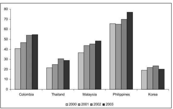
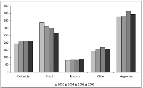
Figure 3.3 and 3.4 compares the general-government-debt-to-GDP ratio of Colombia with a number of selected emerging market economies. It is apparent that both Brazil and the Philippines, with debt-to-GDP ratios of 78.2 and 77.0 percent respectively are in a worse position than Colombia. However, countries like Mexico and Chile in Latin America, and Thailand and South Korea in Asia are in much better positions than Colombia. Malaysia has a similar debt-to-GDP ratio. Argentina is currently in structural default, and has a debt-to-GDP ratio of over 140 percent since the collapse of its fixed-exchange rate system in the end of 2001. The country hopes to restructure its debt to bring down its debt-to-GDP ratio to a manageable level.33

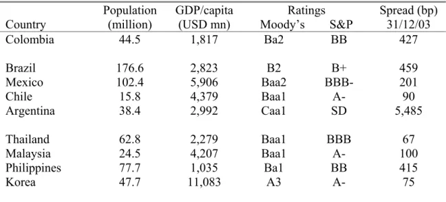
We will in this chapter and the next compare some economic indicators of Colombia with the eight countries in figure 3.3 and 3.4. These countries are presented in table 3.1 together with some selected economic indicators. It is obvious that all the countries, except for South Korea, are middle-income economies.34 The countries do, nevertheless, have very different sovereign credit ratings, and this is also reflected in the spread at which its sovereign debt is trading. Argentina is currently in structural default. Colombia, Brazil and the Philippines have speculative-grade ratings, while the rest of the countries are rated as investment grade.35

32_{According to predictions by Moody’s Investor Service.}

33_{See, for example, Economist (2004) for a recent discussion on Argentina’s restructuring negotiations.} 34_{The commonly used definition of a middle-income country is a country with a GDP per capita between}

USD 1,000 and USD 10,000.

(18)

Figure 3.3: General government debt to GDP, Latin American countries (%)

Note: Argentina is currently in structural default, with a general-government-debt-to-GDP ratio of 146.4 percent in 2002 and 141.2 percent in 2003.

Figure 3.4: General government debt to GDP, Colombia vs. Asian countries (%)

0 10 20 30 40 50 60 70 80

Colombia Brazil Mexico Chile Argentina

2000 2001 2002 2003 0 10 20 30 40 50 60 70 80

Colombia Thailand Malaysia Philippines Korea

(19)

Table 3.1: Selected Latin American and Asian emerging market economies Country Population (million) GDP/capita (USD mn) Ratings Moody’s S&P Spread (bp) 31/12/03 Colombia 44.5 1,817 Ba2 BB 427 Brazil 176.6 2,823 B2 B+ 459 Mexico 102.4 5,906 Baa2 BBB- 201 Chile 15.8 4,379 Baa1 A- 90 Argentina 38.4 2,992 Caa1 SD 5,485 Thailand 62.8 2,279 Baa1 BBB 67 Malaysia 24.5 4,207 Baa1 A- 100 Philippines 77.7 1,035 Ba1 BB 415 Korea 47.7 11,083 A3 A- 75

Source: JP Morgan EMBI Global spread composites, Standard and Poor’s, and Moody’s Investor Service.

Another interesting variable is the total external debt, which includes both public and private debt. The external debt has to be serviced by foreign currency, which comes out of the foreign reserves. In a situation where a country runs out of foreign reserves, it will inevitably default on its external debt. Figure 3.5 and 3.6 compares the external-debt-to-GDP ratio of Colombia with selected emerging market economies. As in the case of the general government debt, the Philippines has a significantly higher external-debt-to-GDP ratio, while Mexico, Thailand and South Korea have lower ratios. Again, Argentina is hopelessly out of line with the rest. An interesting observation is that Chile has an external-debt-to-GDP ratio of as much as 62.9 percent, while its general-government-debt-to-GDP ratio is only 13.5 percent. This is because the private sector has borrowed extensively abroad. This might be a considerable cause of concern if the economy is relatively closed. As discussed earlier, exports are a major source of foreign exchange earnings, and if export earnings are only limited, the country might have problems servicing its external debt. Chile is, indeed, an open economy with a ratio of the sum of exports and imports to GDP standing at 72.4 percent. The corresponding figure for Colombia is 44.2 percent, and for Brazil it is as low as 29.9 percent.

(20)

Figure 3.5: Total external debt to GDP, Latin American countries (%)

Note: Argentina is currently in structural default, with an external-debt-to-GDP ratio of 137.8 percent in 2002 and 114.0 percent in 2003.

Figure 3.6: Total external debt to GDP, Colombia vs. Asian countries (%)

0 10 20 30 40 50 60 70 80

2000 2001 2002 2003 0 10 20 30 40 50 60 70 80

(21)

Even if Chile has a higher external-debt-to-GDP ratio it might be less vulnerable than Colombia, because it is a more open economy. It, therefore, makes sense to look the external debt in relation to exports, or even better, to total current-account receipts.36 Figure 3.7 and 3.8 compares the ratio of external debt to current-account receipts of Colombia and selected emerging market economies. It is apparent from the figure that Chile in this aspect is in a more favourable position than Colombia. In fact, of the countries shown, only Brazil is worse off than Colombia, and of course Argentina. Colombia is, consequently, in a relatively vulnerable position.

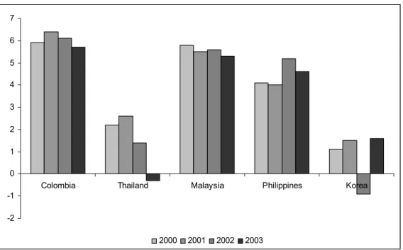
Finally, figure 3.9 and 3.10 graphs the government financial deficit to GDP for the countries studied. If a government runs a large deficit, it might run into problem servicing its debt. For this reason, the government deficit is an important variable when studying emerging market debt. It is apparent from the figures that of the countries studied, only Brazil is worse off than Colombia. Mexico, Chile, Thailand and South Korea are all running low government deficit, and some of these countries have, indeed, run surpluses. The reason for the government surplus in Argentina in 2003 is that the country does not service its debt since it defaulted in end-2001.

(22)

Figure 3.7: External debt to current-account receipts, Latin American countries (%)

Figure 3.8: External debt to current-account receipts, Colombia vs. Asian countries (%)

0 50 100 150 200 250 300 350 400 450

2000 2001 2002 2003 0 50 100 150 200 250 300 350 400 450

Colombia Thailand Malaysia Philippines Korea 2000 2001 2002 2003

(23)

Figure 3.9: Government financial deficit to GDP, Latin American countries (%)

Note: A surplus is here illustrated as a negative deficit.

Figure 3.10: Government financial deficit to GDP, Colombia vs. Asian countries (%)

-1 0 1 2 3 4 5 6 7

2000 2001 2002 2003 -2 -1 0 1 2 3 4 5 6 7

(24)

3.2 Colombia’s Sovereign Spread and Credit Rating

The Colombian sovereign spread, represented by the EMBI Global Colombia composite, is graphed in figure 3.11, for the time period from early 1997 to mid-2004. It is obvious from the graph that the spread during this period was subject to two large shocks. The first of these occurred in late 1998, and was driven by the Russian crisis, induced by the Russian devaluation of the rouble and the default on parts of its outstanding debt in August 1998. This crisis had a huge impact on emerging markets, as illustrated by figure 2.1 in the previous chapter. As for most emerging markets, the impact on the Colombian sovereign spread was severe, as illustrated by figure 3.11.

The second shock occurred in late 2002. This was mainly due to the uncertainty surrounding the Brazilian election in October 2002, when Luiz Ignácio Lula da Silva was elected president of the country. He had, in earlier presidential campaigns, threatened to default on the Brazilian debt, but had this time around committed himself to service the debt fully. Fears of his intentions did, nevertheless, remain, and the Brazilian spread reached almost 2,500 basis points in September 2002. The Brazilian crisis had a severe impact on Colombia spreads, while hardly affecting the sovereign spreads of other emerging markets. The reason why Colombia was so severely affected was the perceived structural similarities of the economies of Brazil and Colombia.37 Both countries had debt-to-GDP ratios of close to 50 percent, and both were running large fiscal deficits. This lead many analysts to conclude that if Brazil defaulted on its debt, Colombia would be forced to do so as well. In late September, the Colombian spread exceeded 1,000 basis points for the first time since the Russian crisis. It was not until the approval of an IMF agreement with Colombia in the end of September, when spreads started falling.

(25)

Figure 3.11: The Colombian sovereign spread 1998 – 2004 (basis points) Source: Rowland (2004b). 0 200 400 600 800 1000 1200 1998 1999 2000 2001 2002 2003 2004 Russia devalues Ruble and halts

foreign debt payments Brazil Real devaluation Ecuador misses scheduled Brady payment September 11 attacks on the U.S. Argentina devalues Peso and defaults

on foreign debt Lula elected president in Brazil Irak war begins Colombian loan packages approved by IMF, IBRD and

IADB Uribe elected president Peace negotiations break down S&P downgraded Colombia to BB S&P downgraded Colombia to BB+ IMF agreement signed Political crisis between the President and

the Congress Colombian Peso floated Earthquake devastated city of Armenia Pastrana elected president IMF rescue package for Brazil announced

(26)

An interesting question is why Colombian spreads were hardly influenced by the Argentina’s sovereign default. In December 2001, Argentina defaulted on USD 132 billion of its debt, by far the largest sovereign default in history.38 This was followed by political chaos on a dimension hard to predict. Fernando de la Rua was replaced as President of the country by Adolfo Rodrigues Saa, who had to resign only a week later after widespread riots and infighting within his Peronist party. Eduardo Duhalde took over the presidency in early January 2002. The Argentine peso, which had been fixed to the U.S. dollar at a parity rate of one to one for over a decade, was devalued. What was to follow was an unprecedented economic collapse. In August 2002, The Economist wrote: “The economic crisis that struck Argentina last year has deepened into one of the worst and most intractable such calamities in living memory”.39 Argentina had, however, been largely decoupled from the rest of emerging markets, and its collapse had little influence on the sovereign spread of other countries, including Colombia.

Colombia is currently rated BB with a stable outlook by Standard & Poor’s and with a negative outlook by Moody’s,40 the two main rating agencies. As stated by Moody’s, this has the following implications:

Bonds, which are rated Ba, are judged to have speculative elements; their future cannot be considered as well assured. Often the protection of interest and principal payments may be very moderate, and thereby not well safeguarded during both good and bad times over the future. Uncertainty of position characterizes bonds in this class.41

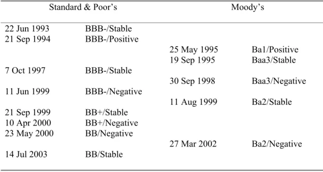
Colombia’s credit rating has, furthermore, been downgraded twice, since it was first rated in 1993, as shown by table 3.2. Colombian was indeed rated investment grade until1999, when it was downgraded to speculative grade by both Standard & Poor’s and Moody’s.42

38_{Economist (2003).} 39_{Economist (2002).}

40_{Colombia is rated Ba2 by Moody’s, which corresponds to the BB rating by Standard & Poor’s. We will}

in this paper use the terminology of Standard & Poor’s unless we specifically refer to Moody’s. The rating systems and terminologies used by the two agencies are summarised in the appendix.

41_{Afonso (2002), p. 4.}

(27)

Table 3.2: Credit rating history of Colombia (long-term foreign currency ratings)

Standard & Poor’s Moody’s

22 Jun 1993 BBB-/Stable 21 Sep 1994 BBB-/Positive 25 May 1995 Ba1/Positive 19 Sep 1995 Baa3/Stable 7 Oct 1997 BBB-/Stable 30 Sep 1998 Baa3/Negative 11 Jun 1999 BBB-/Negative 11 Aug 1999 Ba2/Stable 21 Sep 1999 BB+/Stable 10 Apr 2000 BB+/Negative 23 May 2000 BB/Negative 27 Mar 2002 Ba2/Negative 14 Jul 2003 BB/Stable

Source: Standard & Poor’s, and Moody’s

Other BB-rated countries include Bulgaria, Egypt, Morocco, Panama, Peru and the Philippines. All these countries have, however, traded at tighter spreads than Colombia, as shown by figure 3.12 and table 3.3. Even Peru, which is rated BB- by both Standard & Poor’s and Moody’s, has been trading at a tighter spread.

(28)

Figure 3.12: Sovereign spread of selected BB-rated economies, 2003 average (basis points)

Source: JP Morgan EMBI Global spread composites.

Table 3.3: Sovereign spread of selected BB-rated economies

Country

Ratings Moody’s S&P

Spread

31/12/03 _{Average Max Min Std Dev}Spread during 2003

Colombia Ba2 BB 427 506 706 401 88 Bulgaria Ba2 BB+ 177 228 280 169 25 Egypt Ba1 BB+ 131 204 332 101 64 Morocco Ba1 BB 160 273 399 159 71 Panama Ba1 BB 324 367 451 296 35 Peru Ba3 BB- 325 428 616 277 91 Philippines Ba1 BB 415 453 565 377 50

Source: JP Morgan EMBI Global spread composites, Standard and Poor’s, Moody’s, and own analysis.

427 177 131 160 324 325 415 0 50 100 150 200 250 300 350 400 450

(29)

4 Does Colombia Hold Excessive Reserves?

This chapter analyses the Colombian foreign reserve levels. A project carried out by Banco de la República to estimate the minimum adequate reserve levels of Colombia is presented in section 4.1. Section 4.2 continues by comparing the Colombian reserve levels with those of some other emerging market economies.

4.1 Minimum Adequate Reserve Levels

The main objective of the foreign reserves of a country is to manage the country’s external liquidity as well as to maintain a liquidity buffer that allows time to absorb economic shocks. As illustrated earlier in figure 2.2, the main sources of foreign exchange are exports and foreign investment. If the country at any point in time would deplete its foreign reserves, it would enter a balance-of-payments crisis, where it would be incapable of honouring its external commitments, such as paying for imports or servicing its external debt. In such a situation the country would be forced to default on its external debt, including both public and private debt.

To minimise the risk of a balance-of-payments crisis, a country should always hold certain levels of reserves, which are often referred to as minimum adequate reserve levels. In June 2003, Banco de la República carried out a through project to estimate the minimum adequate reserve levels for Colombia and to investigate the potential gain from using possible excess reserves (i.e. reserves in excess of the minimum adequate reserves) to buy back some of the outstanding sovereign debt.43 The model developed was based on that originally developed by Ben-Bassat and Gottlieb (1992) and is defined in box 4.1.

(30)

Box 4.1. A model to estimate the minimum adequate reserve levels of a country

Let R* be the optimal level of foreign reserves. This R* is the level of reserves that minimise the function of the cost of waiting, C:

C = pC0 + (1 – p) Rr (4.1)

where p is the probability of an external crisis, C0 is the cost of such a crisis as a ratio

to GDP, and r is the opportunity cost of holding foreign reserves. In line with the literature in general, the following functional form was used to represent the probability of an external crisis p:

_f f e e p + = 1 (4.2)

where the exponent f takes the following functional form:

f = α0 + α1 ln(R/A) + α2eD/X + α3m + α4 ln(s) (4.3)

where R is the level of foreign reserves, A is amortizations, D is the total external debt, X is exports, m is the imports-to-GDP ratio, and s is the sovereign spread.

Note: The terminology optimal levels of foreign reserves used by Ben-Bassat and Gottlieb (1992) is in fact here the same as minimum adequate reserve levels.

In June 2003, this model yielded a minimum adequate level of reserves of USD 10.10 billion. Gross foreign reserves were at that time standing at USD 10.50 billion, suggesting that Colombia held excess reserves in the range of USD 400 million. However, when the model was run on data as of March 2004, it yielded an optimal level of reserves of USD 10.69 billion, indicating that relatively small changes in the underlying variables could have a significant impact on the optimal level of reserves. The Bank concluded that Colombia did not hold any significant excess reserves.44

(31)

4.2 Colombian Foreign Reserves in an International Perspective

A relevant question is how the levels of foreign reserves in Colombia are in comparison to other similar emerging markets.45 Figure 4.1 compares the Colombian reserves-to-GDP ratio with those of selected other Latin American countries.46 Relative reserve levels of Colombia are higher than those of Brazil, Mexico and Argentina, but significantly lower than those of Chile. However, it should be noted that Brazil has a lower credit rating than Colombia. Brazil is currently rated B+, compared to Colombia’s BB-rating, and Brazilian sovereign debt is trading at a spread of 459 basis points compared with Colombia’s 427 basis points.47 Argentina is currently in default and does not service its debt. Mexico, on the other hand is rated BBB-, which is two notches above Colombia. It is, however, not as indebted as Colombia. The Mexican total external debt was standing at 27.7 percent of GDP in the end of 2003, while the corresponding debt-to-GDP ratio of Colombia was 47.5 percent.

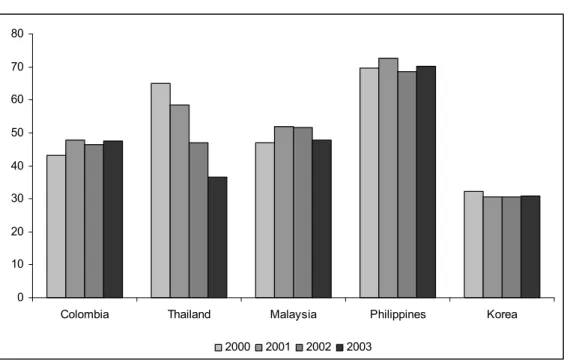
The Asian countries, on the other hand, tend to hold much larger reserves than Colombia. Figure 4.2 shows the reserves-to-GDP ratio of selected Asian emerging market economies in relation to Colombia. Thailand and South Korea are, in relative terms, holding reserves well over twice the Colombian levels, and the Malaysian reserves are standing at over three times the Colombian levels. The fact that Malaysia is holding reserves that are much higher than those of Thailand and South Korea, relatively speaking, can be explained by the fact that the country is maintaining a fixed exchange-rate regime. To do so, a country must hold significant reserves to be able to credibly defend the rate of exchange. Apart from Malaysia, all the other countries in figure 4.1 and 4.2 have floating exchange rates and should, therefore, be directly comparable to Colombia.

45_{The countries selected here are the same as in the previous chapter, i.e. those presented in table 3.1.} 46_{The reserves-to-GDP ratio is better than reserves per capita, since the former take the size of the}

economy into account.

(32)

Figure 4.1: Foreign reserves to GDP, Latin American countries (%)

Figure 4.2: Foreign reserves to GDP, Colombia vs. Asian countries (%)

0 5 10 15 20 25 30 35 40

2000 2001 2002 2003 0 5 10 15 20 25 30 35 40

(33)

An important indicator when analysing the levels of foreign reserves, is the short-term-debt-to-reserves ratio.48 Figure 4.3 and 4.4 illustrates the Colombian short-term debt to GDP in comparison to selected Latin American and Asian emerging market economies. The Colombian short-term debt to reserves is at more or less the same level as the corresponding figure for Brazil. Mexico, on the other hand, has a much lower figure, and Chile stands at a higher level. In the case of Chile, this should not be of too much concern, since Chile is a much more open economy, and a large fraction of the external debt is held by the private sector. Argentina is not really applicable in this comparison, since it has defaulted on its external debt, and is expected to reach a restructuring deal with its creditors.

The Asian economies are, like Chile, much more open than the Colombian economy, and can, therefore, run higher short-term-debt-to-reserve ratios without this being a matter for concern. As shown by figure 4.4, Thailand and Malaysia has short-term-debt-to-reserves ratios below the Colombian level, while the Philippines and South Korea are standing above.

(34)

Figure 4.3: Short-term debt to reserves, Latin American countries (%)

Figure 4.4: Short-term debt to reserves, Colombia vs. Asian countries (%)

Source: Moody’s Investor Service. 0 10 20 30 40 50 60 70 80

2000 2001 2002 2003 0 10 20 30 40 50 60 70 80

(35)

5 Is Colombian Sovereign Debt Undervalued?

The central question in a debt buyback is whether a country, like Colombia, should swap some of the low-risk low-yield securities, in which the foreign reserves are invested, against its own high-risk high-yield sovereign debt. This boils down to the question whether the debt is correctly priced at current market prices or whether it is undervalued, i.e. whether it is a good investment. Section 5.1 discusses this question. In section 5.2 the historical performance of Colombian sovereign debt is analysed, and section 5.3 discusses whether the central bank of a country, Banco de la República in the case of Colombia, might have an advantage when it comes to valuation of the sovereign debt of the country.

5.1 Colombian Bonds versus U.S. T-Bills

A country normally holds its foreign reserves in liquid low-risk foreign government securities. These are normally short-term government bonds from AAA-rated countries such as the United States, the United Kingdom, Germany and Japan. The currency composition of the foreign reserves should, furthermore, reflect the composition of the external trade of the country, to minimise currency risk.

Colombia holds a significant part of its reserves in U.S. Treasury Bills, which are short-term U.S. Government securities, but also in low-risk securities of other countries. Because of the low risk of such securities, they normally offer only limited return.

(36)

Figure 5.1: Return on foreign reserves vs. market yield on Colombian sovereign external debt (%)

Source: Banco de la República

Colombian sovereign bonds, on the other hand, offer a much higher yield, as illustrated in figure 5.1. This is explained by the fact that Colombian sovereign debt is perceived to have a significant risk of default. As discussed in chapter 3, Colombian debt is rated BB by both Moody’s and Standard & Poor’s, which implies that “the protection of interest and principal payments may be very moderate, and thereby not well safeguarded during both good and bad times over the future”.49 To take on this risk, investors demand a significantly higher yield than that offered by low-risk securities, such as U.S. Government bonds. For this reason Colombian sovereign debt trade at a significant spread over U.S. Government debt.

49_{As stated by Moody’s Investor Service when defining Ba-rated debt (equivalent to BB-rated debt of}

0.0 2.0 4.0 6.0 8.0 10.0 12.0 14.0 1997 1998 1999 2000 2001 2002 2003 Period average Return on foreign reserves Market yield on Colombian sovereign bonds

(37)

Figure 5.2: Selling U.S. T-Bills and buying Colombian debt. Changing the composition of the reserves (USD billion)

Note: This graph is only meant to illustrate the principle. The figures in the graph should not be taken as exact numbers.

When studying figure 5.1, on the previous page, it could be argued that Colombia should use any foreign reserves in excess of the minimum adequate reserves to buy back Colombian sovereign debt, since the yield on Colombian debt is significantly higher than on the securities currently held in the reserve. What this would imply is that of the original USD 10 billion or so held in foreign reserves, a part would be invested in Colombian sovereign bonds. This is illustrated in figure 5.2. However, for this to be a good trade, U.S. T-Bills (or the other low-risk securities held in the reserves) must be regarded as expensive relative to Colombian debt. If this would be the case, international mutual funds and other international investors would directly swap their U.S. T-Bills against Colombian sovereign bonds, until prices adjusted, i.e. until the price of Colombian debt rose or the price of U.S. T-Bills fell. However, since international financial markets generally can be considered to be very efficient, both U.S. T-Bills and Colombian sovereign bonds can normally be assumed to be correctly priced.

US T-Bills US T-Bills Colombian debt 0 2 4 6 8 10 Before After

(38)

The reason why the yield on Colombian sovereign bonds are significantly higher than the yield on U.S. Government securities and other investment grade securities is, consequently, the risk involved in investing in Colombian debt. If Colombia does not default, Colombian debt is a better investment. If Colombia, on the other hand, was to default, its sovereign bonds would turn out to be a very bad investment. So it all comes down to the question whether the default risk assigned to Colombian sovereign bonds have been correctly estimated by the financial markets, and, therefore, whether Colombian bonds are correctly priced.

5.2 The Historic Performance of Colombian Debt

One interesting exercise is to study the historic performance of Colombian sovereign bonds. Figure 5.3 illustrates the development of the EMBI Global total return index from early 1997 to mid-2004. This index shows how a portfolio of Colombian sovereign bonds would have developed during different time periods. We can easily see that if we invested in such a portfolio in the beginning of 1997 and sold it in the beginning of 2001, we would not have made any significant profit. In such a case it would certainly have been better to invest in U.S. Government securities instead. However, from the beginning of 2001 and up until the beginning of 2004, with the exception of a temporary fall in mid-2002, Colombian debt was a very good investment. As the sovereign spread of Colombia was decreasing throughout this period (with the exception of the temporary increase in mid-2002) the prices of Colombian bonds have continued to increase steadily. However, Colombian sovereign debt is today trading at a spread that is low relative to historical spreads. It is therefore questionable whether the spread will continue to fall. If the spread starts rising again, this implies that bond prices will fall and, therefore, also that a portfolio of Colombian sovereign bonds will perform badly.

(39)

Figure 5.3: EMBI Global total return index Colombia (28 Feb 1997 = 100)

Source: J.P. Morgan.

This is, nevertheless, only speculation. And a very relevant question is whether the Central Bank of a country or the Ministry of Finance should speculate in its own debt. I will in the next section argue that the Central Bank might have a short-term advantage when it comes to prising the country’s sovereign debt. However, in the long term, the financial markets tend to work efficiently, and the Central Bank might have very little to gain from such long-term speculation. And buyback of debt is certainly a long-term measure.

5.3 Valuation of the Debt: The Central Bank Might Have an Advantage

The Central Bank of a country may have access to information regarding the country’s creditworthiness, and some of this information might not be available to the financial markets. This might either concern information that is confidential and not readily

0 50 100 150 200 250 1997 1998 1999 2000 2001 2002 2003 2004

(40)

available, as well as information that has not yet been released. It might also relate to the fact that the nationals working at the Central Bank tend to know the country better than the often foreign analysts pricing its debt for the international investors. If the Central Bank use this information advantage wisely, it should be able to gain from trading its own debt.

In reality, this has many times turned out to be true in the short term. In August 1998 Russia defaulted on its debt. Many investors believed that the next country to default would be Brazil. In particular, if Brazil would not be able to defend its fixed exchange rate, it would be forced into a default. In mid-January 1999 Brazilian debt traded at a spread over U.S. Government bonds of as much as 1,780 basis points, and in the end of January the country was forced to devalue its exchange rate. Brazil did, however, not default on its debt. The Central Bank at that time knew that the country would avoid a default, and bought back significant amounts of outstanding debt. Three months later, in April 1999, the Brazilian debt traded at a spread below 900 basis points. The Central Bank of Brazil, consequently, made large profits on using its informational advantage over the financial markets.

When it comes to long-term estimation of a country’s default risk, the informational advantage of a Central Bank is much less clear. In the long term the markets tend to have access to more or less the same information as the Central Bank. It could still be argued that the nationals of the Central Bank know the country better than the foreign analysts of international investors. However, this advantage is probably more than counterweighted by the fact that the Central Bank, as a Government institution, has a bias to underestimate the default risk of the country, and the same can certainly be argued for the Ministry of Finance. For this reason it is highly questionable whether the Central Bank is in a better position than the financial markets to estimate the long-term default risk of the country.

(41)

6 How Does a Buyback Affect the Sovereign Spread?

In the previous chapter we discussed whether swapping the low-risk low-yield securities, in which the foreign reserves are invested, against the country’s own high-yield sovereign debt could be considered a good trade. The discussion did, however, not take into account the fact that the Central Bank, which normally manages the foreign reserves, is not like other investors. Even if swapping U.S. T-Bills against Colombian sovereign debt might be regarded as a good trade, it might still not be a good idea for the Central Bank to execute such a trade. Such an operation would decrease the levels of the foreign reserves, which inevitably would have a negative impact on the sovereign creditworthiness of the country, which would generate a rise in the sovereign spread. We will in this chapter analyse this issue further. Section 6.1 presents some conclusions of earlier studies. A cross-country study is carried out in section 6.2. Section 6.3 discusses the Bolivian debt buyback of 1988, which shows that a debt buyback can have perverse consequences unless properly analysed and understood.

6.1 Conclusions of Earlier Studies

Despite the explosive growth of emerging market debt, there have been few studies of the determinants of emerging market sovereign spreads. This is mainly due to the short time series that exist, but also due to the turbulence that these markets have gone through, particularly since the Russian crisis in 1998. Rowland and Torres (2004) present an extensive survey of the literature on the determinants of the sovereign spread and sovereign credit ratings, and this is summarised in table 6.1 and 6.2.50

(42)

Table 6.1. Single-country studies of the sovereign spread Country, Regression Technique and

Data Sample Significant explanatory variables

Budina and Manchew (2000)

Bulgaria Gross foreign reserves (-) Cointegration framework Exports (-)

Monthly data from Jul 1994 to Jul 1998 REER (+)

Mexico’s nominal exchange rate (+)

Nogués and Grandes (2001)

Argentina EMBI total-return index Mexico (-) Estimation technique: Pesaran et al. (2001) External debt service/Exports (+) Monthly data from Jan 1994 to Dec 1998 GDP growth rate (-)

Fiscal balance (-)

30-year U.S. Treasury yield (-)

Rojas and Jaque (2003)

Chile Short-term debt/Reserves (+) OLS regression technique Total external debt/Reserves (+) Monthly data from Apr 1999 to Jul 2002 Exports (-)

Economic activity (-) U.S. Federal Funds rate (+)

Rowland (2004b)

Short-term determinants: EMBI Global spread composite all countries (+) Colombia S&P 500 (-)

OLS regression technique USD/COP exchange rate (+) Daily data (diffs) from Jan 1998 to May 2003

Long-term determinants: Exports (-) Colombia Exchange rate (+) Cointegration framework GDP growth rate (-) Monthly data (levels) from Jan 1998 to Dec 2002 U.S. T-Bill rate (+)

Note: Budina and Mantchev (2000) use the bond price rather than the spread as the dependent variable. They concluded that, in the long run, gross foreign reserves and exports had a positive effect on bond prices, and the real exchange rate and Mexico’s nominal exchange rate depreciation had a negative effect. We have in this table switched the signs on the explanatory variables, to make them comparable to the other studies. If a variable has a positive impact on the bond price, it does, indeed, have a negative impact on the spread, and vice versa.

(43)

Table 6.2. Cross-country studies of the sovereign spread Regression Technique and

Data Sample Significant explanatory variables

Rowland and Torres (2004)

Panel data technique GDP growth rate (-) 16 emerging market sovereign issuers Total external debt/GDP (+) Annual data from 1998 to 2002 Total external debt/Exports (+)

Foreign reserves/GDP (-)

Exports/GDP (-)

Debt service/GDP (+)

Rowland (2004a)

OLS regression on pooled data GDP growth rate (-) 29 emerging market sovereign issuers GDP/Capita (-) Data as of 29 Jul 2003 CPI inflation (+)

Goldman Sachs (Ades et al. (2000))

Panel data technique GDP growth rate (-)

15 emerging market sovereign issuers Total external amortizations/Reserves (+) Monthly data from Jan 1996 to May 2000 Total external debt/GDP (+)

Fiscal balance/GDP (-)

Exports/GDP (-)

REER misalignment (+)

LIBOR (+)

Default history (+)

Eichengreen and Mody (1998)

OLS regression on pooled data Issue size (-) Issue spread, 998 emerging market bonds Private placement (+)

Both corporate and sovereign issues Credit worthiness (Institutional Investors) (-) Period: 1991-1996 Debt/GDP (+)

Debt service/Exports (+)

Min (1998)

OLS regression on pooled data Private issuer (+)

Dummy variable model Total external debt/GDP (+) Issue spread, 505 emerging market bonds Foreign reserves/GDP (-) Both corporate and sovereign issues Debt service/Exports (+) Period: 1991-1995 Growth rate of imports (+)

Growth rate of exports (-) Net foreign assets (-) CPI inflation rate (+) Terms-of-trade index (-)

Nominal exchange rate adjusted by CPI (+)

Maturity (-)

(44)

None of these studies explicitly investigates the relationship between the foreign reserves and the sovereign spread, even if most of the studies conclude that such a relationship exist and has the expected sign.

Most studies in the area are, furthermore, cross-country studies, since many of the fundamental variables determining the sovereign spread only exist with annual frequency. Of the single-country studies, which are listed in table 6.1, Budina and Manchew (2000) find a relationship between the change in the Bulgarian sovereign spread and the change in foreign reserves. Rowland (2004b) does not find any relationship between the Colombian spread and foreign reserves. Nogués and Grandes (2001) do not include foreign reserves in the set of possible explanatory variables studies, and finally, Rojas and Jaques (2003) find both the short-term-debt-to-reserves ratio and the total-external-debt-to-reserves ration to be significant in explaining the Chilean sovereign spread. However, the time series used in all these studies are less than five years long, and it is very possible, that foreign reserves will turn out as a significant explanatory variable in single-country studies when longer data periods are available. The cross-country studies, presented in table 6.2a and 6.2b, give a more conclusive result. Both Rowland and Torres (2004) and Min (1998) finds the reserves-to-GDP ratio to significantly explain the sovereign spread. The paper by Goldman and Sachs (Ades et al. (2000)) finds the total-external-amortizations-to-reserves ratio to be a significant explanatory variable to the sovereign spread. However, neither Rowland (2004a) nor Eichengreen and Moody (1998) find foreign reserves to be a significant explanatory variable.

Interestingly, Rowland (2004a) finds the reserves-to-GDP ratio to be significant in explaining the sovereign credit ratings of both Moody’s and Standard & Poor’s.51 The credit ratings are, furthermore, highly significant in explaining the sovereign spread.

(45)

We will in the next section empirically investigate how foreign reserves influence the sovereign spread of emerging market economies. Theory suggests that a fall in foreign reserves should lead to a rise in the sovereign spread and vice versa. The study in the next section aims to estimate the coefficient of the foreign reserves in the following equation:

EMBIGi = α + βRESi + ui (6.1)

where i = 1, 2, … , N are the number of countries, EMBIG is the spread composite for the individual country, RES is the foreign-reserves-to-GDP ratio, α and β are coefficients to be estimated, and ui is an error term.

The question is whether we can conclude from the cross-country studies presented in table 6.2a and 6.2b what value the coefficient β should be expected to take. The only studies that have estimated the direct relationship between the reserves-to-GDP ratio and the sovereign spread is Rowland and Torres (2004), and Min (1998). Rowland and Torres (2004) obtain a coefficient of -1,051.52 Min (1998), on the other hand, uses a dummy variable model, so these results are not of much help.

52_{Rowland and Torres (2004) used data for the reserves-to-GDP ratio expressed in percent and received a}

parameter estimate of -10.51, which corresponds to -1,051 if the reserves-to-GDP ratio is expressed as an absolute number rather than a percentage.

(46)

6.2 A Cross-Country Estimation

We will in this section investigate the relationship between the sovereign spread and the foreign reserves using a single regression OLS analysis to estimate equation (6.1), which is restated here:

EMBIGi = α + βRESi + ui (6.1)

As before, i = 1, 2, … , N are the number of countries, EMBIG is the EMBI Global spread composite for the individual country, RES is the foreign-reserves-to-GDP ratio, α and β

are coefficients to be estimated, and ui is an error term. As discussed earlier, we use the

EMBI Global spread composite to represent the sovereign spread of a particular country. Table 6.3 shows the dataset used for the empirical study. This is defined by the countries included in the EMBI Global spread composite. Of these countries, Argentina is currently in structural default and is, therefore, trading at an excessive spread, and so is Côte d’Ivoire. These two countries will not be used in the empirical analysis. The data used is, furthermore, from end of December 2003.

(47)

Table 6.3. The dataset used for the empirical estimations Country Ratings Moody’s S&P Spread (bp) 31/12/03 Exchange-rate regime Reserves/ GDP

Argentina Caa1 SD 5,485 Managed float 0.103

Brazil B2 B+ 459 Floating 0.099

Bulgaria Ba2 BB+ 177 Currency board 0.310

Chile Baa1 A- 90 Floating 0.220

China A2 BBB 58 Fixed 0.295

Colombia Ba2 BB 427 Floating 0.125

Côte d'Ivoire Not rated Not rated 3,013 Currency board 0.143

Croatia Baa3 BBB- 122 Managed float 0.295

Dominican Rep B2 CCC 1,141 Managed float 0.018

Ecuador Caa2 CCC+ 799 Dollarized 0.029

Egypt Ba1 BB+ 131 Managed float 0.169

El Salvador Baa3 BB+ 284 Dollarized 0.108

Hungary A1 A- 28 Band 0.145

Korea A3 A- 75 Floating 0.294

Lebanon B2 B- 421 Fixed 0.685

Malaysia Baa1 A- 100 Fixed 0.421

Mexico Baa2 BBB- 201 Floating 0.095

Morocco Ba1 BB 160 Fixed 0.305

Nigeria Not rated Not rated 499 Managed float 0.156

Panama Ba1 BB 324 Dollarized 0.077

Peru Ba3 BB- 325 Floating 0.161

Philippines Ba1 BB 415 Floating 0.166

Poland A2 BBB+ 76 Floating 0.152

Russia Baa3 BB 257 Managed float 0.168

South Africa Baa2 BBB 152 Floating 0.039

Thailand Baa1 BBB 67 Floating 0.286

Tunisia Baa2 BBB 146 Managed float 0.115

Turkey B1 B+ 309 Floating 0.142

Ukraine B1 B 258 Managed float 0.138

Uruguay B3 B- 636 Floating 0.184

Venezuela Caa1 B- 586 Floating 0.196

Note: The EMBI Global spread composite is used to represent the spread of the individual countries.

(48)

Table 6.4. Parameter estimates with the spread as dependent variable

Explanatory Variable Regression 1 Regression 2 Regression 3

Constant 416.60 596.49 970.84 (5.20) (4.64) (4.13) Foreign reserves/GDP -600.45 -1,727.15 -2,698.9 (-1.75) (-2.37) (-1.81) No of observations 29 20 20 Adjusted R2 0.069 0.196 0.108 Standard error 243.8 235.3 468.9

Note: T-statistics are in parentheses.

Table 6.4 presents the results obtained when estimating equation (6.1). Regression 1 uses the full dataset in table 6.3 except for Argentina and Côte d’Ivoire. The parameter for the reserves-to-GDP ratio is of the expected sign but is only significant at the 10-percent level.

Countries with a fixed exchange rate regime can be expected to hold significantly larger reserves than countries with a flexible regime. The reason for this is that countries with a fixed exchange rate need sufficient reserves to defend the exchange rate against speculative attacks. Countries with fixed exchange rates would, therefore, in general be expected to hold larger foreign reserves than countries with a flexible regime, irrespective of their creditworthiness. The average reserves-to-GDP ratio of the countries with a fixed or similar exchange rate regime (currency board arrangement or exchange rate band)53 is 0.360, while for the countries with a flexible regime (floating or managed float)54 is 0.161.

53_{Bulgaria, China, Hungary, Lebanon, Malaysia, and Morocco. As before, the Côte d’Ivoire is not}

(49)

The type of exchange rate regime might, consequently, have a large impact on the level of the foreign reserves. For this reason we re-estimate equation (6.1) with the subset of countries with flexible exchange rate regimes (floating or managed float). The result is presented as Regression 2 in table 6.4. Again the parameter estimate for the reserves-to-GDP ratio is of the expected sign, but this time it is significant at the 5-percent level. The parameter estimate is, furthermore, not that far away from the parameter estimate of -1,051 obtained by Rowland and Torres (2004).

If we rerun the regression with the countries with flexible exchange rates but with data from end-2002 instead of end-2003, we obtain results that are presented in Regression 3 in table 6.4. The parameter estimate of the reserve-to-GDP ratio is of the right sign, but its magnitude is much larger than when using 2003 data. It is, furthermore, only significant at the 10-percent level.

The results of this regression have to be interpreted with some caution. The dataset used include only 20 countries, and those are structurally quite different. The result does, however, suggest that the level of reserves is an important determinant of the yield spread at which a country’s debt is trading.

If Colombia, for example, would use USD 500 million of its foreign reserves to buy back some of its outstanding sovereign debt, this would increase the Colombian sovereign spread by some 85 basis points, according to the results obtained here.55_{Using the results}

obtained with the end-2002 data instead, would yield an increase in the spread of 133 basis points. These figures are in line with the estimates in Banco de la República (2003), which suggest that such a debt buyback would generate an increase in the sovereign spread of 102 basis points.

55_{A reduction of the foreign reserves, from their end-2003 value of USD 10.12 billion, by some USD 500}

million would imply a reduction of 4.94 percent. This multiplied by the coefficient for the reserves-to-GDP ratio of -1.727 yields an increase in the spread of 85.3 basis points.