Method 1668A Interlaboratory Validation Study Report. March 2010

(1)

Validation Study Report

(2)

U.S. Environmental Protection Agency

Office of Water

Office of Science and Technology

Engineering and Analysis Division (4303T)

1200 Pennsylvania Avenue, NW

Washington, DC 20460

(3)

Executive Summary

This report presents the results of EPA’s interlaboratory validation of EPA Method 1668A

Chlorinated Biphenyl Congeners in Water, Soil, Sediment, and Tissue by HRGC/HRMS. This study was conducted in 2003-2004 to validate the performance of EPA Method 1668A in municipal wastewater, fish tissue, and biosolids matrices.

EPA used the results of the study to evaluate and revise Method 1668A quality control (QC) acceptance criteria for initial precision and recovery, ongoing precision and recovery, and labeled compound recovery from real world samples. These interlaboratory criteria (Table 5-1) replace the single-laboratory criteria, and are published in Table 6 of the revised version of this PCB-congener method, EPA Method 1668B.

Acknowledgments

This report was written under contract for EPA by CSC Systems & Solutions, LLC, and Interface, Inc. EPA acknowledges the volunteer laboratories that participated in the study and, in particular, those laboratories that took the extra effort to comment on EPA Method 1668A and to provide suggestions for improvements.

Disclaimer

Mention of trade names or commercial products does not constitute endorsement or recommendation for use.

Contacts

Richard Reding, Ph.D., Chief

Engineering & Analytical Support Branch Engineering and Analysis Division (4303T) Office of Science and Technology, Office of Water U.S. Environmental Protection Agency

1200 Pennsylvania Avenue NW Washington, DC 20460

http://www.epa.gov/waterscience [email protected]

(4)

List of Tables

Table 2-1. Laboratories Participating in the Method 1668A Validation Study

Table 2-2. Congener Concentrations in Wastewater Samples by Level of Chlorination Table 2-3. Sample Pairs for Distribution to 14 Participant Laboratories

Table 3-1. Summary of Data Received from Participant Laboratories

Table 4-1. Congener Concentrations in Study Samples by Level of Chlorination Table 4-2. Congener Concentrations in Blanks by Level of Chlorination

Table 4-3. Wastewater Sample Recovery and Precision by Level of Chlorination Table 4-4. Labeled Compound Recovery and Precision by Level of Chlorination

Table 5-1. Revised QC Acceptance Criteria for IPR, OPR, and Labeled Compounds in Samples

List of Figures

Figure 4-1. Mean Recovery vs. Spike Concentration, PCB Congeners in Wastewater

Figure 4-2. Concentration Standard Deviation vs. Spike Concentration, PCB Congeners in Wastewater Figure 4-3. Relative Standard Deviation vs. Spike Concentration, PCB Congeners in Wastewater Figure 4-4. Mean vs. Standard Deviation of Measured Tissue Results

Figure 4-5. Mean vs. Relative Standard Deviation of Measured Tissue Results Figure 4-6. Mean vs. Standard Deviation of Measured Biosolids Results

(6)

Section 1 Introduction and Background

1.1 Introduction

This report describes the interlaboratory validation study of EPA Method 1668A that EPA conducted in 2003 - 2004 on municipal wastewater, biosolids and fish tissue matrices. The study was conducted according to the Study Plan for Interlaboratory Validation of EPA Method 1668A for Determination of Chlorinated Biphenyl Congeners in Water, Biosolids, and Tissue by HRGC/HRMS,

November 2003, which is an appendix to this report. A draft of this report was peer reviewed, and the following changes were made as a result of this review:

• Rounded all numbers to 3 significant figures maximum.

• Expanded discussion of how QC acceptance criteria were generated

• Moved the definition of “Youden pair” from Section 2.5.1 to its first use in this paragraph.

• Table 4-4: Truncated numbers at the decimal point in the “# pairs” column.

• Section 2.4 was expanded to give greater detail about the nature of the fish and biosolids samples.

• Section 2.5.2 was expanded to give greater detail about how the wastewater sample was prepared.

• A paragraph was inserted into Section 2.7.2 stating that the participating labs were required to determine the solids content of the biosolids sample and report the result in units of dry weight.

• A result in Table 4-1 was corrected.

• Footnote 1 to Table 4-1 was revised to make clear that results for biosolids are in units of dry weight and results for fish are in units of wet weight.

• Footnote 2 to Table 4-1 was revised to state that the mean, median, and maximum concentrations at each LOC are based on any detected congeners in that LOC and when coelution of two or more congeners occurred, the combined value of those co-eluted congeners was used.

• The same Footnote 2 was applied to Table 4-2 because it is called out in the header row. The existing “2” applied to the cell with the number of sand/oil blanks was changed to a “3” in that cell and the existing Footnote 2 was renumbered as Footnote 3.

• Section 4.3 was expanded to clarify that blanks were to be analyzed in the same way as samples.

• The header to column 3 in Table 4-2 was changed from “# labs” to “# blanks” to indicate the number of blanks analyzed in the study.

(7)

• Footnote 1 to Table 4-2 was expanded to indicate that results for the sand/oil blank were to be reported as wet weight.

• Section 4.4 was expanded to explain that, even though the native congeners weren't recovered within the range expected, the labeled congeners were, thus indicating that the native

congeners most likely were lost in transit.

• Table 4-3 was expanded to include recovery and precision for the labeled compounds by level of chlorination

• Section 4.6 and Table 4-4 were expanded to present results for the 27 individual labeled rather than by level of chlorination.

• A fifth footnote was called out in the original Table 5-1, for labeled congeners 156L and 157L, but did not appear below the table. The missing Footnote 5 was added in this version.

EPA used the results of the study to revise Method 1668A and publish, in 2008, Method 1668B. Quality control (QC) acceptance criteria for initial precision and recovery, ongoing precision and

recovery, and labeled compound recovery from real world samples are in Table 5-1 of this report. These interlaboratory criteria replace the single-laboratory criteria, and are published in Table 6 of EPA Method 1668B.

1.2 Background

Method 1668A is for determination of chlorinated biphenyl congeners (PCBs) in water, soil, sediment, biosolids, and tissue by high resolution (capillary column) gas chromatography combined with high resolution mass spectrometry (HRGC/HRMS). These 209 PCB-congeners are the individual chemicals that comprise a class of pollutants known as Aroclors. Since publication in 1999, Method 1668A has been used to measure PCBs in biosolids in EPA’s 2001 National Sewage Sludge Survey, and fish tissue in EPA’s four-year National Study of Chemical Residues in Lake Fish Tissue. Additional background on the nature and determination of PCBs and on the history of development, validation, and peer-review of EPA Method 1668A is in the study plan.

1.3 2003 Revision to Method 1668A

Minor revisions to Method 1668A were made in August 2003 for use in this interlab study. The changes corrected technical and typographical errors and reflected practice of the method by laboratories based on comments received.

(8)

Section 2 Study Management, Objectives, Design, and Implementation

2.1 Study Management

This study was designed and managed by the Engineering and Analytical Support Branch (EASB, formerly the Statistics and Analytical Support Branch) of the Engineering and Analysis Division in the Office of Science and Technology within EPA's Office of Water. Day-to-day coordination of study activities was performed by the contractor-operated Sample Control Center (SCC).1

Preliminary results of this study were presented at the 2004 National Environmental Monitoring Conference in Washington, DC, July 20, 2004. Since that presentation, the results have been further evaluated and presented in this report. Therefore, this report supersedes any material previously presented or published.

2.2 Study Objectives and Design

Objectives of this study were to 1) characterize the performance of Method 1668A in multiple laboratories and matrices, and 2) evaluate and, if appropriate, revise the QC acceptance criteria in the method.

EASB designed the study in accordance with guidelines published by EPA and ASTM International (ASTM).2,3 These guidelines recommend a minimum of six complete data sets for evaluation of a method. To allow for some loss of data due to error, lost samples, outlier removal, or other unforeseen causes, EPA included 14 participant laboratories in the study. The study design is detailed in an appendix to this report.

2.3 Laboratory Selection

EPA used volunteer laboratories for participation in the study. Each interested laboratory was asked to demonstrate that it had recent experience in using HRGC/HRMS to determine chlorinated pollutants in environmental samples and confirm that it would determine all 209 congeners using an SPB-Octyl column, as described in Method 1668A. The intent was to ensure that study participants already possessed the facilities, equipment, and trained staff necessary to implement the method.

Fourteen (14) volunteer laboratories were selected to participate in this study. The laboratories were notified of their selection at least two weeks before the study began, so that they would have time to review the method and study-specific instructions. Of the 14 laboratories selected, 11 were commercial laboratories and 3 were EPA Regional laboratories. Laboratories were not required to validate the method in all three matrices; as a result, the number of participant laboratories varied, depending on the matrix tested. As discussed in section 3 of this report, because of scheduling problems 3 of these 14 volunteer labs did not submit data.

To offset costs to the laboratories, EPA provided each laboratory with a set of analytical standards necessary to identify and measure the 209 PCB congeners targeted by Method 1668A. EPA

1_{The Sample Control Center (SCC) is operated by CSC Systems & Solutions, LLC under contract to EPA.} 2

Guidelines for Selection and Validation of US EPA’s Measurement Methods, U.S. EPA Office of Acid Deposition, Environmental Monitoring and Quality Assurance (OADEMQA), Office of Research and Development, U.S. Environmental Protection Agency, August 1987 Draft.

3

ASTM Standard D2777-98, “Standard Practice for Determination of Precision and Bias of Methods of Committee D-19 on Water,” Annual Book of ASTM Standards, Vol. 11.01, ASTM International, West Conshohocken, PA 19428.

(9)

also provided the laboratories sets of standard solutions containing native and carbon-13 labeled compounds necessary to calibrate their instruments and to conduct all analyses. The packaged sets of standards were purchased from Cambridge Isotope Laboratories (CIL) and AccuStandard, Inc.

Laboratories were provided with detailed instructions for combining and diluting standards to preclude injudicious use of standards. The instructions were based on procedures given in Method 1668A.

In addition to the 14 volunteer participant laboratories, a sample processing laboratory was contracted to perform all activities necessary to ensure that the participant laboratories received

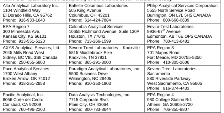
homogenized, spiked, and aliquoted samples. Homogenization of bulk sample volume was necessary to prepare replicate samples for analysis by participant laboratories. The participant and sample processing laboratories are listed in Table 2-1.

Table 2-1. Laboratories Participating in the Method 1668A Validation Study

Alta Analytical Laboratory Inc. 1104 Windfield Way El Dorado Hills, CA 95762 Phone: 916-933-1640 Battelle-Columbus Laboratories 505 King Avenue Columbus, OH 43201 Phone: 614-424-7884

Philip Analytical Services Corporation 5555 North Service Road

Burlington, ON L7L 5H5 CANADA Phone: 800-668-0639 EPA Region 7 300 Minnesota Ave. Kansas City, KS 66101 Phone: 913-551-5120

Columbia Analytical Services

10655 Richmond Avenue, Suite 130A Houston, TX 77042

Phone: 713-266-1599

Enviro-Test Laboratories 9936-67th Avenue

Edmonton, AB T6E OP5 CANADA Phone: 780-413-6481

AXYS Analytical Services, Ltd. 2045 Mills Road West

Sidney, BC V8L 3S8 Canada Phone: 250-655-5800

Severn Trent Laboratories – Knoxville 5815 Middlebrook Pike Knoxville, TN 37921 Phone: 865-291-3000 EPA Region 3 701 Mapes Road Fort Meade, MD 20755-5350 Phone: 410-305-2606 Pace Analytical Services

1700 West Albany Broken Arrow, OK 74012 Phone: 918-251-2858

Paradigm Analytical Laboratories, Inc. 5500 Business Drive

Wilmington, NC 28405 Phone: 910-350-1903

Severn Trent Laboratories – Sacramento

880 Riverside Parkway West Sacramento, CA 95605 Phone: 916-374-4433 Pacific Analytical, Inc.

6056 Corte del Cedro Carlsbad, CA 92009 Phone: 760-496-2200

Data Analysis Technologies, Inc. 7715 Corporate Blvd. Plain City, OH 43064 Phone: 800-733-8644 EPA Region 4 980 College Station Rd. Athens, GA 30605-2720 Phone: 706-355-8807

Note: The primary purpose of this study was to evaluate the performance of Method 1668A. While results obtained by individual laboratories were used relative to this purpose, no attempt was made to assess performance of individual laboratories. No endorsement of these

laboratories is implied, nor should any be inferred. To preserve confidentiality, laboratories that volunteered for this study, including three that did not submit lab data, were assigned numbers randomly from 1 to 14. The lab identities and that of the sample processing laboratory are not revealed in the data or lists in this report.

2.4 Sample Selection

To minimize burden on volunteer laboratories, the study was designed so that no more than two samples of each matrix type would be analyzed, with each sample containing varying concentrations of the target PCB congeners. EPA provided existing (archived) fish tissue and biosolids samples to the sample processing laboratory to prepare study samples representing these matrices. No archived sample volume was available for wastewater, therefore, the sample processing laboratory prepared the

wastewater samples. In preparing study samples, EPA’s objective was to ensure that the congeners present in each sample matrix would span the anticipated measurement range of Method 1668A, from the upper end of the calibration range down to “not detected.”

(10)

Tissue and biosolids samples were generated from excess samples collected during EPA’s 1999-2000 National Lake Fish Tissue Study (NLFTS) and EPA’s 2001 National Sewage Sludge Survey, respectively. These samples had been stored in freezers at an EPA sample repository. All of the tissue samples used in the validation study were from bottom-dwelling fish species and were originally prepared as whole-fish composite samples. The samples for the NLFTS were prepared as finely ground tissue by a single laboratory. Excess sample beyond that shipped to the laboratories during the NLFTS was archived in 500-mL jars and stored frozen. The NLFTS also collected samples of predator species, from which fillets were taken and composited for analysis. The bottom-dweller samples provided more tissue than the predator samples, and thus a greater excess that was available for other purposes such as a Method 1668A validation study. The tissue samples used for the validation study were prepared from the 500-mL archive jars.

The original biosolids samples used to prepare the study samples were collected as solid sewage sludges, as opposed to the pourable liquid sewage sludges that may be produced at some wastewater treatment facilities. Each laboratory that analyzed the biosolids samples determined the percent solid contents. The reported values were in the range of 30 to 40% for the two samples, amounts that are typical for many biosolids produced in the U.S.

So that a sufficient amount of each sample was available to support the study, EPA identified several samples of each matrix type that could be combined to produce large volumes of Youden pairs with the desired congener distribution. (Youden pairs are defined as two samples of the same matrix containing similar, but not exact, concentrations of the analytes of interest.) Once these stored samples were identified, they were forwarded on ice to the sample processing laboratory. Although PCBs are stable and do not require preservation, ice was used to prevent decomposition of fish tissue and to retard gas production in the biosolids. For wastewater, amounts of effluent grab samples were collected from a publicly owned treatment works (POTW) that were sufficient to provide enough samples for all of the participant laboratories, and excess sample in case of breakage, spillage, or other problems. Bulk wastewater was collected in polyethylene carboys and shipped overnight to the sample processing laboratory for spiking and distribution.

2.5 Preparation of Study Samples

The sample processing laboratory was provided with a detailed set of instructions for:

• Combining and homogenizing the biosolids samples

• Combining and homogenizing fish tissues

• The number of aliquots to be prepared from each combined/homogenized matrix

• Aliquoting and spiking the wastewater samples

• Labeling and shipping the prepared sample aliquots.

2.5.1 Biosolids and Tissues

Because the biosolids and tissue samples used in this study were already known to contain PCBs at levels sufficient to cover the analytical range of Method 1668A, the sample processing laboratory did not have to spike these matrices with PCBs. This eliminated concerns about how well spiked constituents would be incorporated into these matrices and whether spiked samples were representative of real-world samples. The goal of the mixing and aliquoting scheme for biosolids and tissues was to obtain Youden pairs for each matrix of interest (i.e., composites A and B). As described in ASTM Practice D2777, the concentrations of Youden pairs should differ by no more than 20%. Because the available “excess” volumes of the biosolids and fish tissues were limited and the number of laboratory participants was relatively large, the Youden pairs were prepared in a multi-step process. For the biosolids, the first step was to combine and homogenize five biosolids samples to form a composite. This composite was then divided approximately in half. One half of the composite was designated as biosolids sample “A” while

(11)

the other half was used to prepare biosolids sample “B.” Biosolids sample “B” was prepared by adding material from a sixth existing biosolids sample, plus some clean sand, to produce a composite with PCB congener concentrations that were approximately 20 % different from those in sample “A.” For the tissue samples, two existing tissue samples were homogenized. The composite was then divided approximately in half, with one half being designated as tissue sample “A.” Tissue sample “B” was prepared by adding tissue from a third existing sample to the remaining half of the initial composite.

The sample processing laboratory was required to perform background and homogeneity analyses of both the biosolids and tissue matrices. The laboratory was instructed to analyze one 10-g dry weight aliquot of sample “A” as the background analysis, and two 10-g dry weight aliquots of sample “B” as the homogeneity aliquots for both the biosolids and tissue matrices. Because of the mixing scheme for both of these matrices, it was assumed that if the homogeneity for sample “B” is found to be acceptable, the homogeneity of sample “A” would also be acceptable. This approach was used to preserve sample mass. Results of tissue and biosolids background and homogeneity analyses are discussed in Section 4.1.

2.5.2 Wastewater

Based on previous experience, municipal wastewater discharges would be unlikely to contain PCB congeners at concentrations sufficient to adequately test the capabilities of the method. Thus, the sample processing laboratory was instructed to first analyze an aliquot of wastewater from a publicly owned treatment works (POTW) to determine background PCB congener levels. Following a review of the background results by SCC, EPA defined the spiking levels, and provided the sample processing laboratory with detailed instructions to divide the unspiked POTW matrix into the required number of aliquots and spike each aliquot separately (rather than spiking a bulk volume of wastewater and then subdividing the spiked sample into replicate aliquots) to the appropriate concentrations. Spiking each aliquot separately avoids problems with “wall effects,” whereby organic pollutants spiked into a bulk sample tend to adhere to the walls of the container, making it difficult to divide a bulk sample into multiple aliquots containing the same analyte concentrations.

In addition, the study-specific instructions provided to each participating laboratory required that the laboratory filter the wastewater sample prior to extraction and treat both the filtrate and any solids on the filter in the manner described in Method 1688A. This instruction was included to prevent problems in which some laboratories followed the method as written, and others deciding to skip the filtration step if the wastewater did not appear turbid.

The unspiked wastewater sample was analyzed by the sample preparation laboratory using Method 1668A. Out of the 209 PCB congeners, 39 congeners were detected in the sample. All of those congeners were between PCB 001 and PCB 168, and all of the concentrations were between 17 and 247 pg/L well below the concentrations of the spikes of the congeners into the wastewater (see Table 2-2 of the Report for the spiking levels). Results for the blanks were all below the calibration range of Method 1668A as practiced by the sample preparation laboratory. The sample preparation lab thus flagged results for the blanks as estimates. In preparing the actual study samples, EPA decided that these background levels were low enough that adjustments need not be made to the amount of each analyte spiked into the samples. The solvent used for spiking the congeners into wastewater was acetone. The volume of acetone used to spike the Youden pair samples was either 0.5 or 0.6 mL per 1-L volume of wastewater.

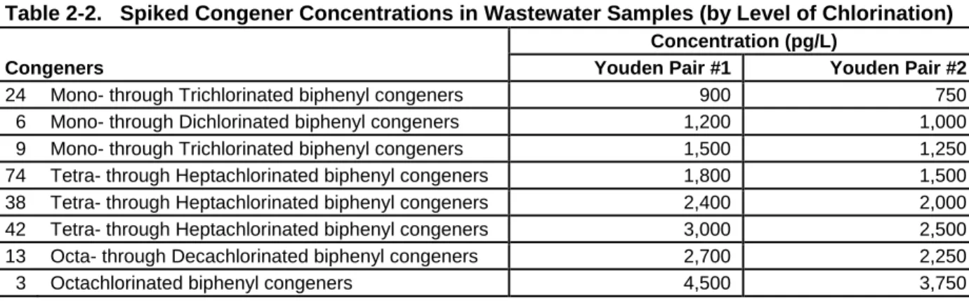
Because of the difficulty that would be encountered in preparing custom spiking solutions, wastewater samples were spiked with varying amounts of “individual native CB congener solutions” A2 through E2 listed in Table 4 of EPA Method 1668A. Concentrations of the congeners in the wastewater samples, by level of chlorination, are given in Table 2-2.

(12)

Table 2-2. Spiked Congener Concentrations in Wastewater Samples (by Level of Chlorination)

Congeners

Concentration (pg/L)

Youden Pair #1 Youden Pair #2

24 Mono- through Trichlorinated biphenyl congeners 900 750

6 Mono- through Dichlorinated biphenyl congeners 1,200 1,000

9 Mono- through Trichlorinated biphenyl congeners 1,500 1,250

74 Tetra- through Heptachlorinated biphenyl congeners 1,800 1,500

13 Octa- through Decachlorinated biphenyl congeners 2,700 2,250

3 Octachlorinated biphenyl congeners 4,500 3,750

The sample processing laboratory analyzed two random aliquots of one concentration level for homogeneity determination. Results of the homogeneity analyses are discussed in Section 4.1.

2.5.3 Labeling and Shipping

SCC provided the sample processing laboratory with a unique 5-digit sample number for each sample. After the aliquots were prepared, the sample processing laboratory labeled each sample container and cap with the corresponding unique sample number. The sample processing laboratory then shipped the prepared, numbered samples to the participant laboratories via air courier. Although PCBs are persistent, and thus do not require preservation, biosolids and tissue samples were shipped on ice to hinder decomposition of the tissues and gas formation in the biosolids. The sample processing laboratory notified SCC of the shipping date, and SCC notified participant laboratories of the shipping and

scheduled arrival dates. Table 2-3 lists the numbers of wastewater, biosolids, and tissue samples that were prepared for distribution to the 14 participant laboratories.

Table 2-3. Sample Pairs for Distribution to 14 Participant Laboratories

Matrix Samples per Laboratory Number of Aliquots Distributed

Wastewater 2 (1 Youden Pair) 28

Biosolids 2 (1 Youden Pair) 28

Tissue 2 (1 Youden Pair) 28

All Three Matrices 6 84

2.6 Sample Analysis and Data Reporting

Participant laboratories did not know the concentration of PCBs in the samples received, and were instructed to prepare and analyze the samples according to Method 1668A procedures, except where stated otherwise in the participant’s scope of work. In addition to the analysis of study samples,

laboratories also were required to prepare and analyze two ongoing precision and recovery (OPR) samples in reagent water, one reagent water blank, and one solids/tissue blank (playground sand mixed with corn oil).

Because study results were to be used to evaluate or further develop QC acceptance criteria, laboratories were prohibited from performing multiple analyses to improve results. Laboratories were, however, allowed to implement corrective action and reanalyses for QC failures attributable to analyst error, instrument failure, or identified contamination. The laboratories also were instructed that any deviations from the method and Statement of Work (SOW) must be pre-approved by EPA.

Laboratories were required to submit electronic and hard copies of summary sample results, and hard copies of all supporting raw data, run chronologies, chromatograms, example equations, and case narratives to SCC for review and data validation. Additionally, laboratories were asked to provide a

(13)

detailed narrative describing any problems or recommendations and a description of any modifications to procedures specified in the method. All submitted data were reviewed against the study and method requirements prior to use for evaluation of method performance. Laboratories were asked to adhere to the following rules in reporting results:

• Report results to the lowest level possible, using a signal-to-noise ratio of 3 as the sample-specific detection limit.

• For congeners that are not detected, report as “<nn”, where nn is an estimate of the detection limit at S/N=3. Do not use the terms “zero,” “trace,” or “ND” (not detection).

• Report PCB congener concentrations in pg/L for aqueous samples or in ng/kg for biosolids and tissue samples.

• Report individual values, including results for congeners found in blanks.

• Do not average or perform other data manipulations unless required by the method or study-specific instructions. Report data to three significant figures, rounding or truncating the data only after all calculations have been completed.

• Report data in the electronic format provided to the laboratory by SCC.

• If data are reported in hardcopy form, paginate all data packages.

2.7 Deviations from the Method or Study Design

Although Method 1668A explicitly allows use of a five-point calibration for less-sensitive instruments (e.g., VG70) and a six point calibration for more-sensitive instruments (e.g., Micromass Autospec Ultima), laboratories interpreted this option differently. This, and other deviations from the study design are described below. Most of these deviations involved use of smaller sample volumes and/or diluted extracts.

2.7.1 Instrument Calibration

Section 10.4 of Method 1668A states that the relative response (RR) (labeled to native) vs. concentration in the calibration solutions should be determined using a five-point calibration for less-sensitive HRMS instruments and a five- or six-point calibration for more-less-sensitive instruments. Laboratories used the following calibration approaches in this study:

• Laboratories 7 and 8 used a six-point calibration (CS-0.2 through CS-5).

• Laboratories 2, 10, and 13 used a five-point calibration (CS-1 through CS-5).

• Laboratory 4 used a six-point calibration with a CS-5 standard at 1/4 the concentration given in the method to prevent saturation of their HRMS instrument.

• Laboratory 12 performed two sets of calibrations, a high and a low. This laboratory applied a high calibration range (CS-1 through CS-5), except in cases where a signal was observed below the CS-1 point, in which case it applied a low calibration range (CS-0.2 through CS-4).

• Laboratory 6 did not provide calibration data.

Provided the instruments were calibrated using a consistent injection volume, these differences in the calibrations used by the laboratories had little or no effect on the results of study samples.

2.7.2 Biosolids

The study-specific instructions stipulated that each laboratory determine the percent solids of the samples, using no more than 2.5 g for that purpose, to ensure that sufficient material was available for several analyses by Method 1668A. The reporting instructions also stipulated that the biosolids results be reported on a dry-weight basis.

(14)

Some laboratories submitted results for the analysis of biosolids samples that: used a smaller sample size than suggested in the method, analyzing more dilute extracts than suggested in the method, or both.

• Laboratory 2 used a 15-g (wet weight) sample as opposed to the 30-g sample suggested by the method, resulting in a two-fold dilution.

• Laboratory 12 used a 6-g (wet weight) sample as opposed to the 30-g sample, resulting in a five-fold dilution.

• Laboratory 7 used a 10-g (wet weight) sample as opposed to the 30-g sample and

concentrated the extract to a final volume of 100 µL, as opposed to 20 µL, resulting in a 15-fold dilution.

• Laboratory 8 used the full sample size, but concentrated the extract to a final volume of 200 µL as opposed to 20 µL, resulting in a ten-fold dilution.

• Laboratory 13 used a 1-g (wet weight) sample as opposed to the 30-g sample, and

concentrated the extract to a final volume of 100 µL as opposed to 20 µL, resulting in a 150-fold dilution. Discussions with this laboratory revealed no attempt to analyze a 30-g sample. Instead, based on past experience with GC/HRMS analyses, the laboratory used a 1-g sample, and concentrated the extract to 100 µL. Their general experience has been that using a 30-g sample results in difficulties during instrumental analysis (lock-mass problems). Based on their GC/HRMS experience, Laboratory 13 also did not use the prescribed sample amounts for the fish tissue and wastewater samples.

Two laboratories (4 and 10) did not submit biosolids data because of difficulties encountered with clean-up and analysis. Both of these laboratories attempted analyses on 30-g samples, as suggested in the method.

Laboratory 4 reported difficulties with the cleanup of both the biosolids samples. In one of the biosolids samples, upon the first acid wash, the sample appeared black in color and the phases could not be distinguished. The laboratory proceeded with the addition of sodium chloride in an attempt to mitigate the problem. During the subsequent acid wash steps (second, third and fourth) no color appeared in the aqueous layer. The extract layer contained suspended particles and had a tar-like appearance and viscosity. The sample was then put through an acid/base silica column before the gel permeation chromatography (GPC) step in hopes that the extract would then not plug the filter used in the GPC. In the case of the second biosolids sample, an emulsion resulted during back-extraction with base (Section 12.5 in the method). The laboratory unsuccessfully attempted to break the emulsion by adding sodium chloride and cooling, and tried diluting the extract with sodium chloride solution and hexane, followed by hexane rinses, and addition of sulfuric acid. The extract was drained into a round bottom flask and concentrated by heating mantle. The sample was then washed with the maximum number (4) of acid washes suggested in the method.

Laboratory 10 reported difficulties with the cleanup and extraction of both biosolids samples and reported that, despite having made two separate attempts to cleanup and extract the biosolids samples, they were not able to obtain reportable results. The samples were initially extracted using approximately 22 grams of each sample (dry weight basis). A total of six cleanup steps were applied to each sample. According to the laboratory narrative, even after these measures, the final extracts contained significant amounts of white crystals. The remaining liquid portions of the extracts were separated from the crystals and injected. These extracts did not yield reportable results. The laboratory attempted to extract the samples a second time, this time using 2 grams each. Two cleanup steps were applied to these samples. No crystals were present in the final extracts; however the laboratory was still unable to obtain reportable results.

Laboratories 7 and 12 reported biosolids results on a wet-weight basis, whereas laboratories 8 and 13 reported biosolids results on a dry-weight basis. The dry-weight data for laboratory 8 were corrected

(15)

to wet weight based on percent solids data provided by laboratory 8 (33.3% solids for Youden 1 and 39.3% for Youden 2). Because laboratory 13 did not provide percent solids data, the laboratory 13 dry-weight data were corrected to wet dry-weight, based on the mean of the percent solids data provided by the: sample preparation laboratory, laboratory 2, and laboratory 8. These three laboratories were the only labs that provided percent solids data (33.3% solids for Youden 1 and 35.9% for Youden 2).

The laboratory narratives suggest that many laboratories lacked experience extracting and cleaning up a biosolids matrix. The resulting deviations from the method and study-specific instructions for analysis of biosolids samples by different laboratories resulted in some unusable and inconsistent data. Thus, EPA excluded some biosolids results, as described in Section 3 of this report.

2.7.3 Tissue

Two of the seven laboratories that submitted usable tissue data used a smaller sample size than that suggested in the method, or analyzed a more dilute extract than suggested in the method.

• Laboratory 7 used a 5-g (wet weight) sample as opposed to the 10-g sample suggested in the method, resulting in a two-fold dilution.

• For reasons similar to their deviation in biosolid sample volume (i.e., previous experience with GC/HRMS analyses), Laboratory 13 concentrated the extract to a final volume of 100 µL as opposed to the 20-µL volume suggested in the method, resulting in a 5-fold dilution. Laboratory 6 did not submit tissue data, and reported difficulties with the analysis of this matrix due to interferences from lipids. The laboratory reported unsuccessful use of an acid-base wash extraction, and two rounds of silica gel cleanup.

2.7.4 Wastewater

One of the eight laboratories that submitted usable wastewater data analyzed a more dilute extract than suggested in the method. Specifically Laboratory 13, for reasons explained previously (GC/HRMS experience), concentrated the extract to a final volume of 100 µL as opposed to the 20-µL volume suggested in the method, resulting in a 5-fold dilution.

(16)

Section 3 Data Review and Validation

Three of the 14 volunteer laboratories that were selected to participate in this study failed to submit data despite repeated requests and offers to extend the submission deadlines. In all three cases, the laboratories cited scheduling conflicts as the reason for their inability to complete the study.

Data from the 11 laboratories that submitted results were reviewed and validated by SCC as soon as possible after receipt. Data packages included sample tracking logs, summary results, QC summaries, raw data, sample calculations, laboratory narratives (including descriptions of any problems encountered, corrective actions taken, and comments on method procedures), and electronic data reporting

spreadsheets. Data were reviewed against requirements in the study plan and the method to ensure that results from each laboratory were complete (i.e., that all required data were present, including results of all required tests, sample lists, run chronologies, summaries of analytical results, raw data, example questions). This included verification that: all samples were analyzed properly; appropriate spike levels were used; the analytical systems were properly calibrated; results calculation procedures were followed correctly; and that raw data supported the results. A fundamental objective of this review was to

maximize data use, and every attempt was made to resolve data discrepancies with laboratories. This review disclosed the following facts:

• Data from Laboratories 3 and 11 failed to meet one or more of the chromatographic

resolution requirements in Section 6.9.1.1.2 of Method 1668A. This section specifies that the SPB-Octyl GC column must resolve congener pairs 34/23 and 187/182, and that congener pair 156/157 must coelute.

• Laboratory 3 data showed coelutions across several chlorination levels, inability to detect many of the congeners in the low (CS-1) calibration standard, and high baseline noise that made integration difficult. Laboratory 3 also reported loss of sensitivity, column

deterioration, and expressed general dissatisfaction with the method. Laboratory 3 reported results for only 1 wastewater sample, 1 blank sample, and no other QC or sample results.

• Laboratory 11 data indicated an inability to recover 25 of the 34 labeled compounds spiked into the biosolids samples without an acknowledgment or explanation of the difficulties, and incomplete raw supporting data. For example, selected ion current profiles for samples in which the laboratory reported very high recoveries of some labeled compounds (e.g., 572%) were not provided. SCC contacted the laboratory repeatedly, but did not receive an

explanation.

• Laboratory 2 submitted only summary level sample results, and provided little or no

calibration data. During attempts to obtain details and raw supporting data, SCC learned that the laboratory manager was no longer with the company and that the laboratory was closing. Without sufficient information to support the summary level results submitted, it was not possible to investigate potential causes of the observed low recoveries. Sample results for this laboratory were consistently below those for all other laboratories, and the labeled compound recoveries were generally low in both study and QC samples.

• Laboratory 6 did not submit tissue sample results and did not provide OPR results associated with the wastewater samples. In e-mail correspondence, the laboratory indicated that the lighter PCB congeners were lost during final transfer, and therefore, results were not submitted. This laboratory provided some raw data (e.g., selected ion current profiles) for some QC samples, but only summary level data for the results of calibration, calibration

(17)

verification, and field samples. SCC was unable to obtain additional information or supporting data. The laboratory reported results for 167 peaks containing one or more congeners. This is more than most other laboratories, and more than the 159 peaks described in the method, making a side-by-side comparison with data from other laboratories difficult.

• Mean relative response (RR) and response factor (RF) values reported by Laboratory 14 were reported inconsistently across the laboratory’s report forms. For example, page 318 of the laboratory’s data package lists the RR for 13C-labeled PCB congener 81 as 2.7956 and page 319 has RR values ranging from 2.01 to 2.28 (with a mean of 2.09). Many of the congeners have only 5 RR values, while many others appear to have 6 RR values. Conversely, for congener 77L, SCC could reproduce the mean RR value of 2.16 reported on page 319, but this value does not match the value of 2.8026 on report Form 3B. Results differ most for the early-eluting labeled congeners. SCC examined the calibration data for these congeners and compared them to calibration data from other laboratories in the study. Although some differences in the responses are expected between different GC/MS instruments, results from Laboratory 14 were inconsistent with results from the other laboratories.

Of the remaining six laboratories:

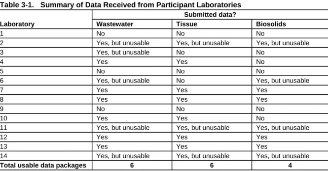
• Four laboratories (7, 8, 11, and 13) provided usable data for all three of the matrices used in this study, and

• Two laboratories (4 and 10) provided usable data for wastewater and tissue matrices only. Thus, this validation study using volunteer labs yielded six usable data sets for wastewater and tissue matrices, and four for biosolids. Data obtained from these laboratories followed the requirements of the study plan and the method and included results for the required accompanying QC analyses; i.e., calibration, calibration verification (where submitted), OPR, reagent water blank, and solids/tissue blank (playground sand mixed with corn oil). Table 3-1 summarizes the status of results from the laboratories.

Table 3-1. Summary of Data Received from Participant Laboratories

Laboratory

Submitted data?

Wastewater Tissue Biosolids

1 No No No

2 Yes, but unusable Yes, but unusable Yes, but unusable

3 Yes, but unusable No No

4 Yes Yes No

5 No No No

6 Yes, but unusable No Yes, but unusable

7 Yes Yes Yes

8 Yes Yes Yes

9 No No No

10 Yes Yes No

12 Yes Yes Yes

13 Yes Yes Yes

Total usable data packages 6 6 4

Study samples were assessed for outlying results using Grubbs’ outlier test, performed in accordance with Standard Practice for Determination of Precision and Bias of Applicable Test Methods of Committee D-19 on Water (ASTM D2777-98). Details on the outlier analyses are presented in Appendix A.

(18)

Section 4 Results and Discussion

4.1 Background and Homogeneity testing

As described in Section 2.3 of this report, the sample processing laboratory was required to perform background analyses of the wastewater matrix, and homogeneity analyses of the tissue and biosolids matrices.

4.1.1 Wastewater Sample Homogeneity

Wastewater samples were prepared: by determining the background concentration to select appropriate spike levels, by spiking and aliquoting the samples as described in Section 2.3, and analyzing two random aliquots for homogeneity verification. Relative percent differences (RPDs) for all congener concentrations between wastewater homogeneity test aliquots B1 and B2 were less than 16%, and all but five were less than 10%, confirming the adequacy of the homogenization and aliquoting process.

4.1.2 Tissue and Biosolids Sample Homogeneity

For tissue and biosolids, the sample processing laboratory was instructed to analyze one 10-g dry weight aliquot of sample “A” as the background analysis, and two 10-g dry weight aliquots of sample “B” as the homogeneity aliquots for both the biosolids and tissue matrices. Because of the mixing scheme for the tissue matrix it was assumed, if the homogeneity for sample “B” was found acceptable, that the homogeneity of sample “A” would be acceptable. This approach was used to preserve mass of sample for the study itself by taking the two homogeneity aliquots from the larger aliquot (sample “B”). Relative percent differences (RPDs) between tissue homogeneity test aliquots B1 and B2 were calculated to verify the homogenization and aliquoting scheme. All but five RPD values were 20%; the remaining five were associated with sample concentrations below the sample-specific minimum level of quantitation (ML; see Table 2 of Method 1668 for MLs), where greater uncertainty is expected.

4.2 Congener Concentrations in Samples

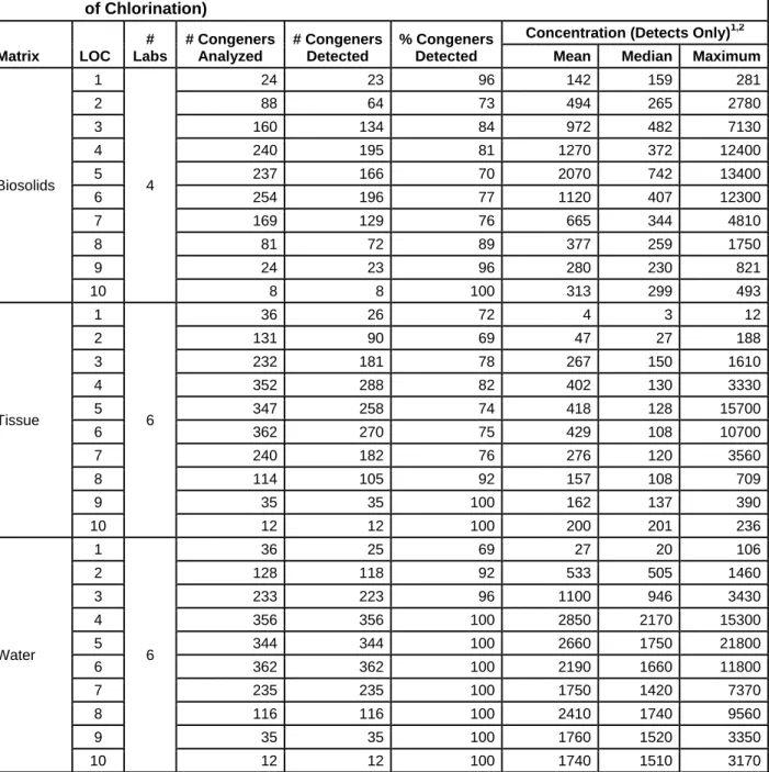
The frequency of detection and the mean, median, and maximum concentrations of the congeners found in tissue, wastewater, and biosolids samples by level of chlorination (LOC) are in Table 4-1. The total number of congeners analyzed reflects the total number of congeners or coeluted congener groups analyzed by all labs in both samples for the given chlorination level. For example, 12 congeners were analyzed in water for LOC 10. This equates to one congener reported by six labs in two samples (12 = 1 x 6 x 2). Although the same six labs provided usable data for tissue and water, there are differences between these matrices in the number of congeners analyzed for a given LOC. For example for LOC 4, a total of 356 tetrachlorinated congeners (or co-eluting congeners) were analyzed in the wastewater Youden pairs, but only 352 tetrachlorinated congeners were analyzed in the in tissue Youden pair. The difference is attributable to the removal of outliers. The next two columns in the table provide information on the number of detected congeners in each LOC, and the percentage of analyzed congeners that were detected. Finally, the mean, median, and maximum concentrations in each LOC represent all congeners within that level; when coelutions of two or more congeners occurred, the combined value of those co-eluted

congeners was used.

In wastewater samples, all congeners at LOCs 4 and higher were detected by all laboratories. Only LOC 1 had a rate of detection below 90%. The rate of congener detection across laboratories was generally consistent for the different LOCs in biosolids and tissue samples, ranging between 69% and 100% for tissue and between 70% and 100% for biosolids. With the exception of LOCs 9 and 10 (which

(19)

include only congeners 3 and 1, respectively), at least one congener was not detected in the solids matrices by at least one laboratory for each LOC. The reason that all laboratories do not detect the same congeners in each sample is likely due to differences in coelutions and because some laboratories concentrated extracts to 100 or 50 µL instead of 20 µL as required by EPA Method 1668A. Those laboratories that did not concentrate extracts to 20 µL would not measure to as low a level as laboratories that did, and low concentration congeners would, therefore, not be detected by these laboratories.

Table 4-1. Congener Detection Rates and Concentrations in Study Samples (by Matrix and Level of Chlorination) Matrix LOC # Labs # Congeners Analyzed # Congeners Detected % Congeners Detected

Concentration (Detects Only)1,2

Mean Median Maximum

Biosolids 1 4 24 23 96 142 159 281 2 88 64 73 494 265 2780 3 160 134 84 972 482 7130 4 240 195 81 1270 372 12400 5 237 166 70 2070 742 13400 6 254 196 77 1120 407 12300 7 169 129 76 665 344 4810 8 81 72 89 377 259 1750 9 24 23 96 280 230 821 10 8 8 100 313 299 493 Tissue 1 6 36 26 72 4 3 12 2 131 90 69 47 27 188 3 232 181 78 267 150 1610 4 352 288 82 402 130 3330 5 347 258 74 418 128 15700 6 362 270 75 429 108 10700 7 240 182 76 276 120 3560 8 114 105 92 157 108 709 9 35 35 100 162 137 390 10 12 12 100 200 201 236 Water 1 6 36 25 69 27 20 106 2 128 118 92 533 505 1460 3 233 223 96 1100 946 3430 4 356 356 100 2850 2170 15300 5 344 344 100 2660 1750 21800 6 362 362 100 2190 1660 11800 7 235 235 100 1750 1420 7370 8 116 116 100 2410 1740 9560 9 35 35 100 1760 1520 3350 10 12 12 100 1740 1510 3170 1

Biosolids (dry weight) and tissue (wet weight) concentrations in ng/kg (pg/g); water concentration in pg/L

2

Mean, median, and maximum concentrations at each LOC are based on any detected congeners in that LOC. When coelution of two or more congeners occurred, the combined value of those co-eluted congeners was used.

(20)

4.3 Congener Concentrations in Blanks

Table 4-2 gives mean, medium, and maximum congener concentrations found in the water and sand/corn oil blanks, by level of chlorination. PCBs can be ubiquitous in the laboratory environment. Congener detection rates in blank samples ranged from 8-33%, with most of the detected congeners being reported at very low concentrations relative to the concentrations reported in samples. The relatively low frequency of detection of congeners in blanks by all laboratories is thought to be attributable to the failure by some laboratories to concentrate extracts to 20 µL and to lesser PCB backgrounds in some

laboratories.

Method 1668A requires that blanks be analyzed in the same way as environmental and IPR/OPR samples, including use of a 1-L aliquot for water or 10 g of an appropriate reference matrix for solids (see Section 7.6 of Method 1668A), and including concentration of extracts of blanks to 20 µL.

Table 4-2. Congener Detection Rates and Concentrations in Blanks (by Matrix and Level of Chlorination) Matrix LOC # Blank samples # Congeners Analyzed # Congeners Detected % Congeners Detected

Concentration (Detects Only)1,2

Mean Median Maximum

Sand/oil 1 103 50 14 28 4.0 3.5 9.6 2 130 20 15 5.3 5.1 12.9 3 227 61 27 2.5 1.4 12.3 4 328 77 23 4.4 2.0 29.0 5 370 70 19 6.7 3.3 37.7 6 355 100 28 5.7 0.4 60.8 7 245 65 27 3.3 0.6 20.0 8 122 30 25 1.3 0.2 5.6 9 50 4 8 2.0 2.1 3.0 10 20 3 15 0.7 0.1 1.9 Water 1 6 30 10 33 25.8 15.1 82.1 2 79 9 11 34.8 21.3 113 3 135 33 24 17.3 11.0 57.7 4 197 43 22 79.5 10.0 2280 5 220 29 13 23.9 20.2 74.2 6 213 52 24 12.2 2.2 85.0 7 146 35 24 6.7 2.5 39.2 8 74 15 20 9.4 9.9 28.4 9 30 3 10 25.4 32.0 33.2 10 12 2 17 13.2 13.2 26.1 1

Sand/oil concentration in ng/kg (pg/g) (wet weight); water concentration in pg/L

2

Mean, median, and maximum concentrations at each LOC are based on any detected congeners in that LOC. When coelution of two or more congeners occurred, the combined value of those co-eluted congeners was used..

3

Six labs provided usable data for sand/oil blanks. Four of the six labs (Labs 7, 8, 10, and 13) analyzed two sand/oil blanks, yielding a total of ten sand/oil blanks.

4.4 Wastewater Sample Recovery and Precision

Table 4-3 summarizes the laboratories’ ability to recover congeners from the wastewater samples, presenting the recovery and precision of congener determination by level of chlorination.

(21)

The mean and median recoveries of nearly all native congeners were in the 60 - 110 percent range, typical for recovery of organic compounds extracted from wastewater. Excluding data at LOCs 1 and 2, the median recovery across all native congeners and all labs is approximately 75%, and the median RSD is approximately 10%. Low recoveries of the native congeners at LOCs 1 and 2 (Table 4-3) may be due to loss during transport from the sample preparation laboratory to the participant laboratories. (Data reported by the sample prep laboratory indicate that the congeners were present immediately after shipment.) Even though the native congeners were not recovered within the range expected, the labeled congeners were recovered from spikes into the wastewater samples by the laboratories. Recoveries of the labeled compounds are shown by LOC in Table 4-3 for comparison. Recovery of the labeled congeners indicates that the loss of the native congeners could not be by evaporation during the solvent evaporation step because the labeled congeners would have been lost also.

The exact reason for loss of the native congeners at LOCs 1 and 2 is not known. Possible causes may be loss by evaporation into the headspace of the sample container during shipment, with subsequent release to the atmosphere when the container is opened, or to biological or other degradation during transit, although selective degradation of congeners at LOCs 1 and 2 only would be unusual. In Figure 4-1, low recoveries for congeners in the 750 - 900 pg/L range are, almost exclusively, attributable to these partial losses of the mono- and dichloro- congeners.

Table 4-3. Wastewater Sample Recovery and Precision by Level of Chlorination

LOC

Percent Recovery (%) Within-pair Relative Standard Deviations (%)

# Results Mean Median Min. Max. # Pairs Pooled* Median Min. Max.

Native congeners spiked by sample prep lab

1 25 3.15 2.71 0.49 11.8 11 29.7 17.5 5.8 80.8 2 118 54.2 44.6 2.63 162 57 12.2 4.42 0.17 62.4 3 223 89.5 82.8 34.2 164 111 7.62 5.06 0.02 24 4 356 95.6 91.4 38.1 201 178 7.36 6.16 0 20.6 5 344 81.4 72.2 30.6 182 170 10.8 7.99 0.06 40.5 6 362 75.3 68.8 8.14 196 178 12.1 8.64 0.16 46.8 7 235 72.3 64.4 10.4 155 114 9.63 5.24 0.14 39.3 8 116 68 59.3 18.1 135 56 11.3 7.26 0.12 32.3 9 35 70.8 57.8 44.4 126 17 8.91 6.66 0.57 18.5 10 12 70 59.1 49.3 118 6 5.67 4.23 0.37 9.05

Labeled congeners spiked by participant labs

1 24 51.4 48.9 21.0 84 12 19.7 13.8 3.45 42.9 2 24 58.5 55.1 25.0 90 12 15.7 11.9 0 29.2 3 36 67.4 62.6 26.0 108 18 12.5 5.32 0.516 33.3 4 33 60.5 57.5 35.0 101 15 8.24 3.34 0.873 17.7 5 83 77.2 81.0 41.0 110 41 11.0 2.61 0 28.7 6 50 75.6 74.3 38.6 106 25 9.83 7.13 1.32 21.8 7 36 76.9 77.0 5.00 123 18 30.4 3.72 0 126 8 23 76.6 79.5 38.4 94 11 6.20 5.12 2.29 12.4 9 24 71.2 70.0 49.1 98 12 6.33 4.24 0 9.92 10 12 73.1 74.5 52.8 98.2 6 6.81 5.26 4.07 12.0

* Pooled RSD calculated as the square root of the mean of the squared within-pair RSDs

Recovery, as a function of concentration, is plotted in Figure 4-1. (Plots of absolute and relative precision as a function of concentration are addressed with precision for biosolids and tissue samples in

(22)

Section 4.5.) The spike concentrations displayed in Figure 4-1 do not match exactly the concentrations that were spiked (see Table 2-2) because coelutions result in combined concentrations.

Figure 4-1. Mean Recovery vs. Spike Concentration, PCB Congeners in Wastewater

4.5 Variability as a Function of Concentration

Because true congener concentrations in the tissue and biosolids samples were not known, it was not possible to calculate recoveries of congeners from tissue and biosolids. Variability (precision) vs. concentration was determined for wastewater, soil, and, tissue matrices. The following subsections present plots of absolute precision (as standard deviation of the determined concentrations) and relative precision (as relative standard deviation) as functions of congener concentration for each of these matrices. For the three matrices, standard deviation increased approximately linearly with increasing concentration. It was expected that, at the very low concentrations in the tissue and biosolids samples, standard deviation would become constant and the plots would resemble a “hockey stick.” (The

wastewater sample was not spiked at low enough concentrations to demonstrate this effect.) The lack of a hockey stick appearance for the tissue and biosolids; i.e., the lack of constant standard deviation at low concentrations, is good because this indicates that measurements are being made in the quantitative range for the congeners. This is not surprising because the rigorous congener identification criteria in Method 1668A are that the signal-to-noise ratio must be greater than 3 and ratio of the peak heights or areas for the 2 exact m/z’s must be within 15% of theoretical, in addition to the requirement that the relative retention time of the congener must be within a specified window based on a calibration or calibration verification standard. Thus, the identification criteria raise the lowest level of congeners that are determined to levels above the region of constant standard deviation.

4.5.1 Variability vs. Concentration for Wastewater

4.5.1.1 Absolute variability vs. concentration for wastewater

Figure 4-2 is a plot of the standard deviation as a function of concentration for the congeners spiked into wastewater. The congener concentrations are defined by the spiking solutions, as described in Section 2.5.2. Results appear slightly skewed to lower standard deviation at low concentration. The skewed appearance is likely due to the higher concentrations of the coeluted congeners.

(23)

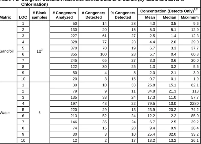
Figure 4-2. Concentration Standard Deviation vs. Spike Concentration, PCB Congeners in Wastewater

4.5.1.2 Relative variability vs. concentration for wastewater

Figure 4-3 is a plot of RSDs as a function of concentration for the congeners spiked into wastewater. The congener concentrations are defined by the spiking solutions, as described in Section 2.5.2. The variability is somewhat higher than expected at the higher concentrations, with RSDs of approximately 40%. The reason for these higher than expected RSDs is not known.

Figure 4-3. Relative Standard Deviation vs. Spike Concentration, PCB Congeners in Wastewater

(24)

4.5.2 Variability vs. Concentration for Tissue

4.5.2.1 Absolute Variability vs. Concentration for Tissue

Figure 4-4 is a plot of standard deviation as a function of concentration for congeners detected in tissue. Congeners were detected in tissue from as low as a few parts-per-trillion (ppt; pg/g) to well into the part-per-billion (ppb; ng/g) range.

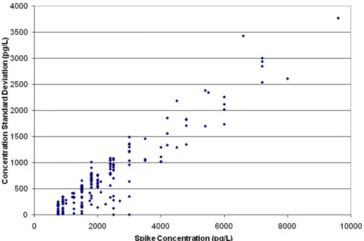
Figure 4-4. Mean vs. Standard Deviation of Measured Tissue Results 4.5.2.2 Relative Variability vs. Concentration for Tissue

Figure 4-5 is a plot of RSD as a function of concentration for the congeners detected in tissue. RSDs are mostly between 10 and 30 percent, as expected, with a few outlying high values. The unusually high RSDs occurred in congeners that are only rarely detected (2-3 laboratories.)

(25)

Figure 4-5. Mean vs. Relative Standard Deviation of Measured Tissue Results

4.5.3 Variability vs. Concentration for Biosolids

4.5.3.1 Absolute Variability vs. Concentration for Biosolids

Figure 4-6 is a plot of standard deviation as a function of concentration for congeners detected in biosolids. Congeners were detected in biosolids from as low as a few ppt to well into the ppb range.

Figure 4-6. Mean vs. Standard Deviation of Measured Biosolids Results

.5.3.2 Relative Variability vs. Concentration for Biosolids 4

Figure 4-7 is a plot of RSDs as a function of concentration for the congeners detected in biosolids. Unlike the plots of relative variability for tissue and wastewater samples, this plot does not

(26)

suggest a strong relationship between variability and concentration. RSDs are mostly between the expected ranges of 10 to 30 percent, with a few outlying high values.

Figure 4-7. Mean vs. Relative Standard Deviation of Measured Biosolids Results 4.6 Labeled Compound Recovery and Precision

Table 4-4 lists labeled compound recovery and precision for the 27 labeled congeners spiked into wastewater, biosolids, and tissue samples. Except for congener 1L, median recoveries ranged from 56 to 94 percent. Except for congener 178, pooled RSDs ranged between 5 and 22 percent. The low recovery of congener 1L and, to some extent other congeners at low chlorination levels, is thought to be caused by loss in the solvent evaporation step. The reason for the high RSD for congener 178 is not known. Table 4-4. Recovery and Precision of Labeled Compounds Spiked into Samples1

LOC2

Labeled Congener3

Recovery (%) Within-pair RSD (%)

# Results Mean Median Min. Max. # Pairs Pooled4 Median Min. Max.

1 1L 32 52.9 48.5 13.0 95.0 16 22.0 17.4 0.81 43.4 1 3L 32 60.4 61.1 15.9 107 16 18.9 10.9 2.70 47.6 2 4L 32 60.8 56.1 32.0 120 16 16.7 11.9 1.30 31.6 2 15L 32 64.8 69.0 25.0 96.3 16 13.7 2.8 0 31.4 3 19L 32 59.0 59.0 4.5 112 16 12.0 5.4 0.69 26.5 3 28L 32 78.8 87.8 25.0 118 16 11.7 7.8 1.40 33.3 3 37L 32 77.2 77.6 35.0 110 16 10.0 2.4 0.52 23.6 4 54L 31 61.6 59.1 25.5 109 15 10.3 5.4 0.87 22.0 4 77L 31 72.7 67.3 43.0 106 15 9.1 5.7 1.10 19.8 4 81L 31 74.9 71.0 26.0 129 15 9.0 6.6 1.30 18.8 5 104L 32 76.5 80.0 41.0 102 16 10.1 4.8 0 24.4 5 105L 31 81.9 86.3 52.7 103 15 10.9 5.2 0.50 25.2 5 111L 29 85.2 86.3 63.0 110 13 5.4 3.7 0.29 12.7 5 114L 32 83.0 86.3 48.0 119 16 10.8 5.2 1.00 28.3 5 118L 32 83.9 87.5 53.8 120 16 10.8 6.4 0.36 26.6 5 123L 32 84.7 88.8 53.8 116 16 11.4 6.5 0.48 23.4

(27)

Table 4-4. Recovery and Precision of Labeled Compounds Spiked into Samples1

LOC2

Labeled Congener3

Recovery (%) Within-pair RSD (%)

# Results Mean Median Min. Max. # Pairs Pooled4 Median Min. Max.

5 126L 32 81.0 80.8 59.0 123 16 11.8 4.5 0 28.7 6 155L 32 77.3 81.3 33.0 106 16 7.8 3.6 0 21.8 6 156L+157L 32 87.8 76.5 44.0 216 16 12.9 8.0 1.10 30.3 6 167L 31 84.3 82.0 57.3 110 15 9.9 8.6 1.30 22.6 6 169L 32 78.3 75.3 30.5 112 16 14.8 8.0 2.40 37.5 7 178L 30 89.1 93.8 5.0 126 14 34.6 4.7 0.69 126 7 188L 32 78.0 85.2 32.0 136 16 8.5 4.6 0.22 17.4 7 189L 32 82.8 82.0 54.0 118 16 8.1 4.8 0 18.2 8 202L 31 84.9 87.8 38.4 145 15 9.2 5.4 1.30 19.9 8 205L 32 82.3 81.5 51.0 118 16 7.9 4.8 0.25 17.3 9 206L 32 80.8 81.3 50.0 115 16 9.2 7.7 0 19.8 9 208L 32 80.4 84.7 49.0 129 16 7.6 4.9 0 17.2 10 209L 32 78.7 79.8 47.7 110 16 9.2 6.3 2.20 18.9 1

Wastewater, biosolids, and tissue

2

Level of chlorination

3

Labeled analog of World Health Organization dioxin-like (Toxic) congener shown in bold

4

(28)

Section 5 Revision of Quality Control Acceptance Criteria

Interlaboratory quality control (QC) acceptance criteria were developed for initial precision and recovery (IPR), on-going recovery (OPR; laboratory control sample, LCS), and for recovery of labeled compounds from samples. These revised criteria are in Table 5-1 of this report, and Table 6 of the successor method, 1668B. The statistical details for development of these criteria are in an appendix to this report. The tests to which these criteria are applied are discussed in this Section of this report.

5.1 Calibration

The study plan and study-specific instructions suggested a 5- or 6- point calibration. Laboratories did not provide enough calibration data to permit revision of the QC acceptance criterion for calibration linearity. Therefore, the criterion for which an average relative response may be used for a given congener remains at 20%, as stated in Section 10.4.4 of EPA Method 1668A; otherwise, a calibration curve must be used for that congener. This calibration linearity criterion applies to congeners determined by isotope dilution only (i.e., the “toxics,” “level of chlorination,” and “GC window-defining” congeners) because all other congeners are calibrated at a single point.

5.2 Calibration Verification

The study plan and study-specific instructions suggest single calibration verification after

calibration. Because only two laboratories submitted calibration verification data, EPA did not revise the calibration verification QC acceptance criteria. The calibration verification QC acceptance criteria in Table 5-1 remain unchanged from previous revisions of EPA Method 1668A. If EPA receives calibration verification data from enough laboratories, EPA may revise these criteria in future versions of 1668.

5.3 Initial Precision and Recovery

To minimize resource burden on volunteer participants, laboratories were not required to prepare and analyze IPR samples. Instead, EPA used the OPR data gathered in the study to develop revised IPR and OPR QC acceptance criteria. In addition, results from the aqueous and solids (sand/corn oil) OPRs were combined to yield a single set of OPR QC acceptance criteria that would be applicable to aqueous, solids, and tissue samples. Two laboratories resolved labeled and native congeners 156 and 157, while the other laboratories reported these congeners as coeluting pairs. Similarly, one laboratory reported coelution of congeners 4 and 10, one laboratory reported coelution of congeners 114 and 122, and two laboratories reported congener 106 coeluting with either congener 107 or 109. Because calculations of IPR/OPR QC acceptance criteria were based on recoveries, coelution was ignored when generating the revised criteria.

Data from Laboratories 2, 3, 6, 11, and 14 were excluded for the reasons described in Section 3 of this report. The remaining dataset yielded a total of 15 usable reagent water and solid matrix OPR

samples. After performing Grubbs' outlier tests on these OPRs, a total of 13 individual data points were identified as outliers and removed from the dataset prior to development of revised IPR/OPR QC acceptance criteria. Table 5-1 presents revised IPR QC acceptance criteria. When compared to QC acceptance criteria in Method 1668A, recoveries windows are generally narrower than those in the method. Recoveries for low molecular weight congeners are centered lower than for the other congeners and for recoveries of low molecular weight congeners in Method 1668A. These lower recovery windows reflect that these congeners are partially lost in the solvent evaporation step(s).

(29)

QC acceptance criteria for IPR precision, as relative standard deviation (RSD) of recoveries, are also presented in Table 5-1. The RSDs generally are higher than those in Method 1668A for some of the low molecular weight congeners, and lower for some of the other congeners. The higher RSDs for the low molecular weight congeners reflect partial loss of these congeners in the solvent evaporation step(s) in Method 1668A, resulting in greater variability in results for these congeners.

5.4 Ongoing Precision and Recovery

Each participating laboratory was required to spike and analyze two reagent water OPR samples. These samples were used to evaluate laboratory and method performance and to update IPR and OPR QC acceptance criteria. Although not required by the study design, four laboratories analyzed at least one solids matrix OPR sample. In some cases, laboratories provided one solids matrix OPR and one reagent water OPR instead of two reagent water OPRs. In other cases, laboratories supplemented the two reagent water OPRs with one or more solids matrix OPRs.

Revised OPR QC acceptance criteria are in Table 5-1. As with the IPR QC acceptance criteria, OPR recovery windows are, generally, narrower than those in Method 1668A, and centered lower for some of the low molecular weight congeners.

5.5 Labeled Compound Recovery from Samples, Blanks, and IPR and OPR standards

Labeled compound recovery data from samples were used to construct revised QC acceptance criteria for labeled compound recoveries. Results from a total of 24 analyses were used to develop the labeled compound recovery QC acceptance criteria (Table 5-1.) The IPR and OPR recovery windows are centered lower, for the low molecular weight congeners.

(30)

Table 5-1. Revised QC Acceptance Criteria for IPR, OPR, and Labeled Compounds in Samples Congener Congener number1 Test conc. (ng/mL)2 IPR _OPR Recovery (%)3

Labeled Compound Recovery in Samples and Blanks (%)3 RSD (%) Recovery (%)3 2-MoCB 1 50 25 84 – 119 71 – 132 NA 4-MoCB 3 50 22 83 – 112 72 – 123 2,2'-DiCB 4 50 18 82 – 105 73 – 114 4,4'-DiCB 15 50 17 85 – 107 76 – 116 2,2',6-TrCB 19 50 13 86 – 103 79 – 109 3,4,4'-TrCB 37 50 26 77 – 109 64 – 122 2,2',6,6'TeCB 54 50 17 84 – 106 76 – 114 3,3',4,4'-TeCB 77 50 20 81 – 106 71 – 116 3,4,4',5-TeCB 81 50 20 81 – 106 70 – 116 2,2',4,6,6'-PeCB 104 50 19 83 – 107 74 – 117 2,3,3',4,4'-PeCB 105 50 19 83 – 107 73 – 117 2,3,4,4',5-PeCB 114 50 18 83 – 105 74 – 113 2,3',4,4',5-PeCB 118 50 13 88 – 105 81 – 112 2',3,4,4',5-PeCB 123 50 16 82 – 102 74 – 109 3,3',4,4',5-PeCB 126 50 17 82 – 104 74 – 113 2,2',4,4',6,6'-HxCB 155 50 15 86 – 105 79 – 112 2,3,3',4,4',5-HxCB4 156 50 16 87 – 108 78 – 117 2,3,3',4,4',5'-HxCB4 157 50 16 87 – 108 78 – 117 2,3',4,4',5,5'-HxCB 167 50 13 85 – 101 79 – 107 3,3',4,4',5,5'-HxCB 169 50 16 80 – 100 73 – 108 2,2',3,4',5,6,6'-HpCB 188 50 14 88 – 106 81 – 113 2,3,3',4,4',5,5'-HpCB 189 50 16 85 – 106 77 – 114 2,2',3,3',5,5',6,6'-OcCB 202 50 17 82 – 104 74 – 112 2,3,3',4,4',5,5',6-OcCB 205 50 15 87 – 107 79 – 115 2,2',3,3',4,4',5,5',6-NoCB 206 50 17 85 – 106 76 – 115 2,2',3,3,'4,5,5',6,6'-NoCB 208 50 17 86 – 108 77 – 116 DeCB 209 50 20 81 – 106 71 – 116 Labeled Compounds 13 C12-2-MoCB 1L 100 78 21 – 100 2 – 100 4 – 100 13 C12-4-MoCB 3L 100 63 31 – 100 13 – 100 11 – 106 13 C12-2,2'-DiCB 4L 100 56 35 – 100 18 - 100 14 – 107 13 C12-4,4'-DiCB 15L 100 70 34 – 100 10 – 118 19 – 107 13 C12-2,2',6-TrCB 19L 100 68 32 – 100 10 – 106 1 – 108