Performance of diagonal control structures at different operating
conditions for Polymer Electrolyte Membrane Fuel Cells
Maria Serra (corresponding author), Attila Husar, Diego Feroldi, Jordi Riera Institut de Robòtica i Informàtica Industrial
Universitat Politècnica de Catalunya - Consejo Superior de Investigaciones Científicas C. Llorens i Artigas 4, 08028 Barcelona, Spain
e-mail: [email protected]
telephone: 34 93 4015789; fax: 34 93 4015750
ABSTRACT
This work is focused on the selection of operating conditions in Polymer Electrolyte Membrane Fuel Cells. It analyses efficiency and controllability aspects, which change from one operating point to another. Specifically, several operating points that deliver the same amount of net power are compared, and the comparison is done at different net power levels. The study is based on a complex non-linear model which has been linearised at the selected operating points. Different linear analysis tools are applied to the linear models and results show important controllability differences between operating points. The performance of diagonal control structures with PI controllers at different operating points is also studied. A method for the tuning of the controllers is proposed and applied. The behaviour of the controlled system is simulated with the non-linear model. Conclusions indicate a possible trade-off between controllability and optimisation of hydrogen consumption.
Keywords: PEMFC, diagonal control, linear control, PI controllers, operating conditions, linear analysis, efficiency
1. INTRODUCTION
Compared to other types of fuel cells, Polymer Electrolyte Membrane Fuel Cells (PEMFC) have many advantages that make them suitable for a large number of applications: high power density, compactness,
lightweight, low-operating temperature, solid electrolyte, long cell and stack life, low corrosion, and high efficiencies [1]. However, important difficulties remain unsolved and a lot of research is being done in order to make the technology ready to implementation and commercialisation [2].
The operating conditions for PEMFC have been described in the literature [3]. However, a comparison of the system controllability at different operating points is not found. A PEMFC can deliver the same amount of net power at different operating conditions. In order to chose the appropriate operating point, control aspects have to be taken into account, as well as efficiency aspects. Some works address the control of PEMFC [4][5][6], but only the efficiency is considered to determine the operating conditions. The objective of this work is to compare the controllability of a PEMFC operated at different operating conditions. The performance of the control system is evaluated implementing a diagonal structure with PI controllers in the control loops.
2. THE MODEL
In their study of the PEMFC flow dynamics, Pukrushpan et al. presented a control oriented model for an automotive application which has been the base for the model used in this work [7]. The transient phenomena captured in the model include the flow and inertia dynamics of the compressor, the manifold filling dynamics (both anode and cathode), reactant partial pressures, and membrane humidity. On the other hand, the model neglects the extremely fast electrochemical and electrical dynamics, and temperature is treated as a constant parameter because its slow behavior (time constant of 102 sec) allows it to be regulated by its own controller. A
constant cell temperature of 80 ºC is assumed.
Mass and energy balance are the basic laws for the different volumes being modeled. Constant properties are assumed in all volumes. Flowrates from one volume to another are calculated as a function of the upstream and downstream pressures. Ideal gases are assumed as well as the same properties of the gases exiting one volume and these gases inside the volume.
Membrane hydration captures the effect of water transport across the membrane. Water transport is due to drag and diffusion effects. Both water content and mass flow are assumed to be uniform over the surface area of the membrane.
Stack voltage is calculated as a function of stack current,cathode pressure, reactant partial pressures, fuel cell temperature, and membrane water content.
The air entering the cathode is impelled by a compressor the model of which consists of a dynamic part and a static part read from an experimental compressor map. The modelled compressor has the angular velocity limited
to 100 kRPM, the exit flow limited to 0.1 kg/sec, and the pressure ratio limited to 4. The power consumed by the compressor is the only parasitic power taken into account. The net power is therefore calculated as the electric power given by the fuel cell minus the power consumed by the compressor. Cooler and humidifier are also included. It is assumed that a static humidifier supplies the air with the desired relative humidity before entering the stack.
At the anode side, entering hydrogen comes from a pressurized tank and the hydrogen flow is assumed to be a manipulated input variable.
Only one modification is introduced, which is the introduction of an anode exit flow. This exit is necessary to control the hydrogen pressure along the flow channels and to improve the power demand transient responses [2]. Some of the indexes used for the linear analysis depend on the model scaling. One of the controlled outputs is the difference of pressure between anode and cathode, Δp. It has been scaled with a variation of 0.1 bar. To scale the rest of the input and output variables, a maximum variation of 10% has been assumed. Hence, the scaled variables are the non-scaled increments divided by the maximum increments.
SIMULINK linearisation tools have been used to obtain the state space matrices of the system at the studied operating points.
3. OPERATING CONDITIONS
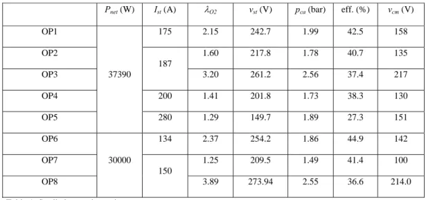
This work is based on the analysis of a set of selected operating points. Their operating conditions are summarized in Table 1. In Figure 1, the operating points are located on the curves of net power versus stoichiometry at different current values. In a fuel cell, a certain amount of net power can be obtained at different currents. OP1 to OP5 deliver the same net power (Pnet=37400 W), and the same happens with OP6 to OP8, with
Pnet=30000 W. OP1 and OP7 have the minimum amount of current for which Pnet of 37400 W and 30000 W can
be respectively obtained. For example, it is not possible to obtain 37400 W of net power with a current lower than 175 A, at any pressure or stoichiometry. These operating points are specially interesting because minimum current corresponds to the minimum hydrogen consumption if the hydrogen that does not react is assumed to be recycled. Looking at the different curves of Figure 1, it can be seen that Pnet increases when λO2 increases for
small λO2, but this trend changes from a certain λO2 value. This is because when λO2 is high, to increase λO2
requires a compressor power increase larger than the electric power increase obtained from the fuel cell. Therefore, operating points with the same net power and current are possible (i.e. OP2 and OP3, or OP7 and OP8). It will be interesting to compare these two operating conditions with different stoichiometries that deliver
the same net power with the same hydrogen consumption.
4.CONTROL OBJECTIVES
In this work, the stack current is considered a disturbance and there is a desired stack voltage which depends on the required power. Therefore, the first control objective is to maintain vst to the setpoint value. On the other
hand, in order to prevent membrane damage, the difference in pressure between anode and cathode Δp needs to be small [8]. A small Δp will favour the membrane life time, and thus, the second control objective is to maintain
Δp close to zero.
For certain applications, the required power is constant and there is a unique voltage setpoint. The selection of this setpoint (selection of operating conditions) is the main issue concerning this work. However, if the range of required power is large, different setpoint voltages will be necessary (even a desired operating curve), and what are the appropriate operating conditions will be questioned at every power level.
5. STRUCTURE OF THE CONTROL SYSTEM
The control structure analysed in this work consists of a decentralised PI based controller. Two output variables are controlled using two of the input manipulated variables giving a 2×2 control problem. The input control variable chosen to control vst is vcm. This control loop is called the first loop. To control Δp, Wan_in has been
chosen. This is called the second loop. From all possible pairs of manipulated variables, vcm and Wan_in have been
chosen because this is what is found in the literature [4, 5, 6] and what is recommended after a controllability analysis by Serra et al. [9].
6. TUNING OF PI CONTROLLERS
In order to compare the behaviour of the proposed control structure at different operating points, it is important to employ the same tuning methodology. In this section, a tuning methodology is proposed.
For the first loop, the control of vst, Ziegler-Nichols tuning rules can be applied [10]. However, they are not
appropriate for the second loop, the control of Δp, because they provoke sudden changes in pressure that could damage the membrane. The tuning method used for the second loop introduces a parameter that has been used to limit the pressure peaks. The tuning procedure consists of the following steps:
a) Tuning of the first control loop. This tuning has been done with some tuning rules that can be viewed as a modification of the Ziegler-Nichols step response method: the Kappa-Tau tuning procedure [11]. These
rules use three parameters to characterise the process dynamics instead of two, permitting substantial improvements in control performance while retaining much of the simplicity of the Ziegler-Nichols method. b) Tuning of the second control loop. The transfer function that relates Δp with Wan_in is of second order, but
has a zero and a pole which almost cancel each other. Eliminating the zero and pole, an equivalent first order transfer function is obtained. The methodology employed was proposed by Rivera et al. for disturbance rejection of low-order processes [12]. The PI parameters Kc and Ti are Kc=τ/(λ*kp) and Ti=T. In this case, λ has been chosen such that Δp peaks are no larger than 0,3 bar when current steps of 40 A/s and giving power increments of ±20% are applied.
Applying this tuning methodology to OP1, OP2, OP3, and OP5, the tuning parameters indicated in Table 2 are obtained.
7. LINEAR ANALYSIS
MIMO linear systems can be analysed using different analysis tools. These tools are mathematic operators applied to the transfer functions of the linear system. Some of them are applied to the process (without control) and characterise the controllability of the system as a property of the process itself. Others are applied to the controlled system and depend on the control structure and tuning. In this work, the following indexes and matrixes are considered in order to study the performance and controllability of the system: the Morari Resiliency Index (MRI), the Condition Number (CN), the Relative Gain Array (RGA), the sensitivity function, S, and the complementary sensitivity function, T.
The MRI is the smallest singular value of the open-loop transfer function. It is the poorer gain of the process, poorer sensitivity, which corresponds to specific input and output directions. Large MRI over the frequency range of interest are preferred. The CN is the ratio of the maximum singular value to the minimum singular value. It indicates the sensitivity balance in a multivariable system. Large CN indicate unbalanced sensitivity and also sensitivity to changes in process parameters. Therefore, small CNs are preferred. The RGA matrix is used to determine the interaction among control loops in a multivariable process. It is defined as the ratio of the open-loop gain for a selected output when all the other open-loops of the process are open, to its open-open-loop gain when all the other loops are closed. Pairings that have RGA close to unity matrix at frequencies around bandwidth are preferred. This rule favours minimal interaction between loops and prevention of stability problems caused by interaction. Contrarily, large RGA elements indicate sensitivity to input uncertainty. S is a good indicator of the closed loop performance [13]. Typical specifications in terms of S include a large bandwidth frequency (large
frequency where the maximum singular value of S crosses 0.707) and a small peak of its maximum singular value. Large peaks indicate poor performance as well as poor robustness. Finally, T can be used to analyse the stability of the MIMO system [14]. The criterion require that the maximum value of its maximum singular value is small for robust stability. This maximum peak criterion can be insufficient for MIMO systems for which advanced tools considering uncertainty descriptions (μ-analysis) are needed. However, to have an idea of the stability robustness, this analysis can be useful.
The frequency range of interest is given by the bandwidth frequency, normally defined as the frequency up to which control is effective [13]. It is assumed that the bandwidth will not be larger than 103 rad/s. In Figures 2, 3 and 4, the MRI, CN and RGA(1,1) of the 2X2 system are plotted. The three controllability indexes indicate the same trends: comparing OP1, OP2, OP4, and OP5, the controllability improves when the current increases. OP5 has the highest MRI, the lowest CN and the RGA closest to 1, followed by OP4, OP2, and OP1. Comparing these operating points with OP3, results indicate the poorest controllability at OP3. It can be seen that differences remain important all long the analysed frequency range.
If the analysis is repeated at a different Pnet level, 30000W, similar results are found: OP7 has better
controllability than OP6, and OP8 has the poorest controllability of the three.
The sensitivity function, S, and the complementary sensitivity function, T, are also calculated for the controlled system at OP1, OP2, OP4, and OP5 using the tuning parameters indicated in Table 2. The maximum and minimum singular values of these matrixes are shown in Figures 5 and 6. Similar conclusions can be deduced from both Figures: the controlled system is faster at OP5, and the peaks are lower for OP5, indicating better performance and robust stability. Therefore, from a control point of view, OP5 is the best, followed by OP4, OP2, and OP1.
8. SIMULATION RESULTS
In order to take into account the influence of the nonlinearities, different simulations are done with the non-linear model. Figures 7 to 14 show the behaviour of the controlled system in front of current and voltage setpoint step changes. Simulations are done around OP1 and OP5. All the combinations of 0 and ±10% increments in Ist and vst
setpoint are applied, covering eight equidistant directions of the bidimensional space defined by these two inputs. The dashed lines correspond to the ±10% current increments. Figures 7, 9, 11, and 13 correspond to operation around OP1, and Figures 8, 10, 12, and 14 correspond to operation around OP2.
confirms a lower system directionality at OP2. Comparing Figures 7 and 8, while similar vst peaks are found, a
faster control is obtained at OP2. The worst oscillations are found at OP1. Looking at Δp, peaks are larger at OP1. In Figures 11 and 12, it can be seen that vcm has much larger increments and oscillations around OP1. Finally, in
Figures 13 and 14 a better behaviour is found around OP2 as well, with faster response, smaller peaks, and less oscillations.
To analyse the controlled system behaviour in front of larger disturbances around OP1 and OP2, current steps of –24% and +30% (corresponding to ±20% of net power) have been applied. Simulations show a similar behaviour of vst and Δp at the two operating points, but both vcm and Wan,in have larger peaks at OP1.
Therefore, simulation results agree with the linear analysis that the analysed fuel cell system has better control properties at OP2. Moreover, for the analysed variables and within the scope of this work, it can be said that the performance of the proposed control system around OP2 is satisfactory.
9. CONCLUSIONS
Using three different controllability indexes (the MRI, the CN, and the RGA) to compare the controllability of a PEMFC at different operating points, it has been found that the higher the efficiency, the lower the controllability. Having done the comparative analysis at different net power levels, it can be said that the conclusion is valid in a wide operating range. When comparing operating points with the same current and net power, but different output voltage, the operating points with higher stoichiometry have the worst controllability. Also, some performance tools (the sensitivity function S and T) indicate that it is easier to control the system when it is operated at the operating point with lower efficiency. Finally, some simulations are done, which show the same trend. Therefore, comparing the controllability and performance of a controlled PEMFC at different operating conditions, it has been found that there is a trade-off between controllability and efficiency within a wide operating region. In this work a diagonal control structure for a PEMFC is analysed. PI controllers are implemented in the control loops and a tuning procedure has been proposed. For the analysed variables and within the scope of this work, it can be said that the performance of the proposed control system around OP2 is satisfactory. The size of the compressor appears to have a key influence over the controllability of the system at different operating points.
NOMENCLATURE
Kc Proportional constant of the PI controller
Kp Steady state gain of the process
Pnet Net power (W)
Ti Time parameter of the PI controller (s)
Wan,in Anode inlet mass flow rate (kg/s)
ifc Fuel cell current density (A/cm2)
pca Cathode pressure (bar)
vst Stack voltage (V)
vcm Compressor voltage (V)
λ Parameter of the controller
λO2 oxygen stoichiometry
ACKNOWLEDGMENT
This work has been funded partially by the projects CICYT DPI2002-03279 and CICYT DPI2004-06871-C02-01, of the Spanish Government
REFERENCES
[1] L. Carrette, K. A. Friedrich, U. Stimming, Fuel cells - Fundamentals and applications, Fuel Cells 1, 1, 2001
[2] W. Yang, B. Bates, N. Fletcher, R. Pow, Control challenges and methodologies in fuel cell vehicle
development, International Congress of Transportation Electronics 98C054, 1998
[3] J. Larminie, A. Dicks, Fuel Cell Systems Explained, John Wiley & Sons Ltd, 2003
[4] J. Pukrushpan, A. G. Stefanopoulou, H. Peng, Control of fuel cell breathing, IEEE Control Systems
Magazine, April 2004
[5] M. Grujicic, K. Chittajallu, J. Pukrushpan, Control of the transient behaviour of polymer electrolyte membrane fuel cell systems, Proceedings of the Inst. Mech. Engrs. Vol. 218 Part D: Journal of Automobile Engineering, 2004
[6] A. Vahidi, A. Stefanopoulou, H. Peng, Model Predictive Control for prevention starvation in a hybrid fuel cell system. Proceedings of the American control conference, Vol. 1 pp.834-839, 2004.
[7] J. T. Pukrushpan, H. Peng, A. G. Stefanopoulou, Control-oriented modeling and analysis for
automotive fuel cell systems, Transactions of the ASME, vol. 126, March 2004
[8] S. Yerramalla, A. Davari, Dynamic modelling and analysis of polymer electrolyte fuel cell, IEEE 2002 [9] M. Serra, J. Aguado, X. Ansede, J. Riera, Controllability analysis of decentralised linear controllers for polymeric fuel cells, Journal of Power Sources, Article in press.
[11] K. Astrom, T. Hagglund. PID controllers: Theory, Design and Tuning, ISA 1995
[12] D. Rivera, S. Skogestad and M. Morari. Internal model control 4: PID controller design. Ind. Eng. Chemical Process Design Dev., 25, 252-265, 1986.
[13] S. Skogestad, I. Postlethwaite, Multivariable Feedback Control, Analysis and Design, John Wiley & Sons 1996
[14] W. Luyben. Process modeling, simulation and control for chemical engineers, 1990.
TABLES:
Pnet (W) Ist (A) λO2 vst (V) pca (bar) eff. (%) vcm (V)
OP1 37390 175 2.15 242.7 1.99 42.5 158 OP2 187 1.60 217.8 1.78 40.7 135 OP3 3.20 261.2 2.56 37.4 217 OP4 200 1.41 201.8 1.73 38.3 130 OP5 280 1.29 149.7 1.89 27.3 151 OP6 30000 134 2.37 254.2 1.86 44.9 142 OP7 150 1.25 209.5 1.49 41.4 100 OP8 3.89 273.94 2.55 36.6 214.0
Table 1: Studied operating points
OP1 OP2 OP4 OP5 1st loop 2nd loop 1st loop 2nd loop 1st loop 2nd loop 1st loop 2nd loop
Kc 10.28 1.72 6.41 0.87 4.81 0.94 1.91 1.80
Ti 0.22 3.32 0.22 3.84 0.22 3.89 0.22 3.46
Table 2. Scaled PI tuning parameters
0.5 1 1.5 2 2.5 3 3.5 4 4.5 5 0 1 2 3 4 5 6x 10 4 λO2 Pnet (W) OP6 OP8 OP3 OP7 OP1 OP2 OP5 OP4 Ist=280 Ist=250 Ist=220 Ist=200 Ist=187 Ist=175 Ist=134 Ist=2150 10-2 10-1 100 101 102 103 10-6 10-5 10-4 10-3 10-2 10-1 100 101 Frequency (rad/s) MR I OP1 OP2 OP3 OP4 OP5 OP6 OP7 OP8
Figure 1. Different operating points Figure 2. MRI at the different operating points
10-2 10-1 100 101 102 103 100 101 102 103 104 Frequency (rad/s) CN OP1 OP2 OP3 OP4 OP5 OP6 OP7 OP8 10-2 10-1 100 101 102 103 0.7 0.75 0.8 0.85 0.9 0.95 1 Frequency (rad/s) RG A (1 ,1 ) OP1 OP2 OP3 OP4 OP5 OP6 OP7 OP8
Figure 3. CN at the different operating points Figure 4. RGA at the different operating points
10-1 100 101 102 103 -60 -50 -40 -30 -20 -10 0 10 20 Frequency (rad/s) σ (S ) OP1 OP2 OP4 OP5 10-2 10-1 100 101 102 103 -100 -80 -60 -40 -20 0 20 40 Frequency (rad/s) σ (T ) OP1 OP2 OP4 OP5
49.5 50 50.5 51 51.5 52 52.5 53 200 210 220 230 240 250 260 270 Time (s) vst ( V o lts ) 49.5 50 50.5 51 51.5 52 52.5 53 120 130 140 150 160 170 180 Time (s) vst ( V o lts )
Figure 7. vst response at OP1 Figure 8.vst response at OP2
49.5 50 50.5 51 51.5 52 52.5 53 -0.2 0 0.2 0.4 0.6 0.8 Time (s) Δ p (b ar ) 49.5 50 50.5 51 51.5 52 52.5 53 -0.2 0 0.2 0.4 0.6 0.8 Time (s) Δ p (b ar )
Figure 9.
Δ
p response at OP1 Figure 10.Δ
p response at OP249.5 50 50.5 51 51.5 52 52.5 53 -50 0 50 100 150 200 250 300 350 400 Time (s) vcm (V o lt s ) 49.5 50 50.5 51 51.5 52 52.5 53 60 80 100 120 140 160 180 200 220 240 Time (s) vcm (V o lt s )
49.5 50 50.5 51 51.5 52 52.5 53 0.5 1 1.5 2 2.5 Time (s) W an ,in ( g /s ) 49.5 50 50.5 51 51.5 52 52.5 53 0.5 1 1.5 2 2.5 Time (s) W an ,in ( g /s )