Electric Distribution Network Multiobjective Design
Using a Problem-Specific Genetic Algorithm
Eduardo G. Carrano, Luiz A. E. Soares, Ricardo H. C. Takahashi, Rodney R. Saldanha, and Oriane M. Neto
Abstract—This paper presents a multiobjective approach for the design of electrical distribution networks. The objectives are defined as a monetary cost index (including installation cost and energy losses cost) and a system failure index. The true Pareto-op-timal solutions are found with a multiobjective genetic algorithm that employs an efficient variable encoding scheme and some problem-specific mutation and crossover operators. Results based on 21- and 100-bus systems are presented. The information gained from the Pareto-optimal solution set is shown to be useful for the decision-making stage of distribution network evolution planning.
Index Terms—Decision-making, energy distribution networks, genetic algorithms (GAs), multiobjective optimization, network topology optimization.
I. INTRODUCTION
O
PTIMIZATION techniques should be employed for the design of engineering systems, allowing for the best allo-cation of the limited financial resources. In electrical energy sys-tems, most of the electrical energy losses occur in the distribu-tion systems. Most of the energy supply interrupdistribu-tions also occur due to faults in this subsystem. Due to its large extension, the designer of the distribution system often tries to keep its instal-lation cost as low as possible, which often leads to lossy and un-reliable systems. Moreover, the nature of a distribution system expansion, which is done inherently by small incremental steps which occur at the same time in different geographical locations, and at the same location at different times, does not favor the ap-plication of efficient design methodologies. Particularly, if the expansion is performed in small fragments of the system, the overall combinatorial possibilities of network topologies may not be fully considered, which can result in a system that is more expensive, less reliable, and more lossy than a globally designed one.This paper presents a tool that can be used both for the de-sign of a new distribution system and for the resizing of an ex-isting system, occasionally adding some new nodes. A multiob-jective approach is used, considering the following: i) the finan-cial costs that appear due to system installation, system mainte-nance, and energy losses; and ii) the costs that are incurred due Manuscript received December 16, 2004; revised May 17, 2005. This work was supported in part by CAPES, in part by CNPq, and in part by Fapemig. Paper no. TPWRD-00593-2004.
E. G. Carrano, R. R. Saldanha, and O. M. Neto are with the Departamento de Engenharia Elétrica, Universidade Federal de Minas Gerais, Belo Horizonte MG 30123-970, Brazil.
L. A. E. Soares is with Strike Engenharia e Consultoria, Belo Horizonte MG 30160-010, Brazil.
R. H. C. Takahashi is with the Departamento de Matemática of Universidade Federal de Minas Gerais, Belo Horizonte MG 30123-970, Brazil.
Digital Object Identifier 10.1109/TPWRD.2005.858779
to system faults (undelivered energy and restarting procedures). The importance of considering, in the design stage, the issue of system reliability is discussed in [1] and [2]. Those references consider, as the objective to be minimized, a weighted sum of the financial costs and the fault costs.
Although those costs can both be measured in monetary units, they represent different dimensions that should not be added to form a single scalar cost. This fact can be understood if one notices that an electric utility company should prefer spending a certain amount of money with any operational cost than spending the same amount of money as a result of system faults that lead to nondelivered energy, increased maintenance costs, and fines imposed due to service interruption. Therefore, the same amount of money, spent in financial costs and fault costs, represents different costs that should not be aggregated in a single “cost” variable. The suitable framework for the analysis of an optimization problem with more than one objective is the multiobjective optimization, which can lead to meaningful results that would not be reached with mono-objective methods. This paper presents a true multiobjective approach for dealing with the described problem.
A multiobjective genetic algorithm (GA) is employed here as an optimization tool. In recent years, it has been recognized that GAs are particularly well suited for multiobjective optimization problems since they can simultaneously evolve an entire set of multiobjective solutions (the Pareto-optimal solutions). In this way, instead of running an optimization algorithm once a time for finding each point of such a set, the GA can find this set in a single run [3], [4].
The problem of designing the topology of a network is con-sidered to be a difficult combinatorial optimization problem [5], [6]. It has been recognized that deterministic algorithms, such as branch-and-bound methods and dynamic programming, are unable to solve such problems beyond the scale of medium-size networks [7], [8]. This has motivated most of the recent works related to this problem to employ some kind of randomized op-timization algorithm [2], [8]–[17]. Most of the algorithms em-ployed in such references are GAs. GAs structured in the con-ventional way, however, would be inefficient for solving this class of problems [6]. References [8] and [14] have noticed the inadequacy of conventional GAs for this problem, and use a GA with conventional operators plus a local search operator, which is based on mathematical programming techniques.
In this work, another kind of problspecific GA is em-ployed: the proposed algorithm uses the problem structure of a planar tree graph for building efficient genetic operators (crossover and mutation operators) that allow genetic popula-tion diversity and avoid solupopula-tion infeasibility (adopting a kind 0885-8977/$20.00 © 2006 IEEE
of solution “fixing”). A peculiarity of the problem structure is also exploited here in order to allow a description that reduces the problem order of complexity. This paper is presented as follows.
• Section II discusses the fundamental differences between the mono-objective and the multiobjective optimization approaches in a generic framework.
• Section III presents the problem to be dealt with: the ob-jective functions and the constraints and the description of the network design problem.
• Section IV discusses the structure of genetic multiobjec-tive algorithms.
• Section V presents the specific multiobjective GA that is proposed here.
• Section VI shows the results of application of the proposed algorithm to two test systems.
• Section VII deals with the decision-making process in this specific problem.
II. MONO-OBJECTIVEVERSUSMULTIOBJECTIVEAPPROACH Conventional mono-objective optimization is stated as the problem of finding the point, in a space of optimization vari-ables, in which a certain function (the objective function) reaches its minimum value. The multiobjective optimization problem, instead of looking for a single point, searches for a set of points, the Pareto-optimal set, which is the set of optimal solutions of a problem with more than one objective function [18]. The Pareto-optimal set is defined in the following.
Consider the minimization of a vector function
(the vector of problem objective functions) in which the set represents the problem feasible set. There is not, in gen-eral, a single point in which reaches the minimum value for all of its components. Then
such that
and (1)
in which the relational operators and are defined for vectors as
for some (2)
The points that do not belong to the set are said to be dominated since there are some other points so that
and , which means that is better
than in at least one coordinate, without being worse in any other coordinate. In this case, dominates . The solutions that belong to the set are called the efficient solutions, since they are not dominated by any other point1. Therefore, the
multiobjective optimization looks for the efficient solutions of a problem of vector optimization. The concept of a Pareto set,
1Notice that the efficient points all have objective coordinates that are not
worse in comparison with the coordinates of the nonefficient points that they dominate, but not necessarily in comparison with the coordinates of all nonef-ficient points. The feature that determines a point being nonefnonef-ficient is that it is dominated by some efficient point, not by all efficient points.
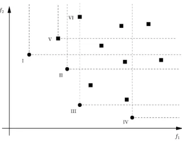
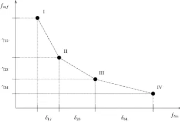
Fig. 1. Consider an optimization problem of discrete optimization variables with a finite number of possible values. All possible instances of the optimization parameters of a biobjective vector optimization problem have their two objectivesf ( 1 )andf ( 1 )evaluated. Each evaluation corresponds to a point in thef 2 f plane, as shown in the figure. The points marked with circle (points I to IV) are the efficient solutions, and the points marked with square are the dominated points. Note, for instance, that the point I dominates point VI, with both of its objectivesf andf being smaller than point VI ones. Point III also dominates VI, having only objectivef smaller, and objectivef equal to the point VI one. Note that although point V dominates point VI too, point V is not an efficient solution, since point V is also dominated by point I. Note also that, although point IV is an efficient solution, it does not dominate point VI: although its objectivef is smaller, its objectivef is greater than the point VI one. The solutions I to IV are efficient because they are not dominated by any other solution, while the other solutions are dominated, since they are worse or equal, in all objectives, than at least one solution of the Pareto set (I to IV).
for a discrete variable optimization problem (which is the case for the network topology optimization problem) is illustrated in Fig. 1.
Finding the whole set is a useful analysis tool in a system design procedure, since the relative position of the elements of this set gives the information about the existing tradeoff among the problem objectives. This means that the designer can eval-uate the effect of replacing a solution by another one, in terms of loss in some objective with simultaneous enhancement in an-other objective. The mono-objective approach does not allow for such analysis.
Often, when faced with a problem in which a vector of objectives should be minimized, the system designer employs the approach of aggregating the objectives in a single cost index
that weights the different objective functions
(3) However, it can be shown that such an approach is not suitable for generating the whole Pareto set . Even if the designer tries to scan the set by varying the weights , some solutions which belong to this set cannot be found. For instance, solution II in Fig. 1 which is not in the boundary of the convex hull of the feasible set mapping, would not be found by the weighting
method [18]. Therefore, a true multiobjective optimization al-gorithm should be employed for finding the elements of the Pareto set .
III. DISTRIBUTIONNETWORKDESIGNPROBLEM The energy distribution network is represented by a planar tree graph (radial structure). The possible connections between the nodes (paths where the conductors can be placed) are the optimization variables in this kind of problem. They are discrete variables that can only assume 0 (the branch does not exist) or a positive integer value (describing the branch type used between two nodes). In addition to the active network, a small number of initially inactive branches are placed. These inactive branches define alternative paths that are to be used when a failure breaks down an active branch, in this way avoiding, at least partially, the energy supply interruption that would occur in such cases. These are the reserve branches.
The optimized design of distribution networks must consider four main objectives.
• minimization of energy losses;
• minimization of investment in new facilities and distribu-tion lines;
• minimization of the average number of faults; • minimization of average interruption time in faults. Besides, some constraints should also be considered:
• line capacity;
• voltage level in load buses;
• graph connectivity and radiality of the active network
( , where is the number of branches and
is the number of nodes); • quality and reliability index.
An important feature of the objective functions considered here is the strong interaction they present between the changes in network topology (the topology must also satisfy a constraint of radiality) and the changes in the type of conductors to be used in each connection. This precludes the application of very simple algorithms for solving the problem, such as algorithms that first find the “optimal topology,” and then the “optimal con-ductor set” for that topology. The GAs are included among the algorithms that are suitable to deal with this kind of problem [19].
The earliest approaches to this problem have just considered the reduction of cost as objective, minimizing the investment in new facilities and energy losses. More recent studies have con-sidered the reliability of the electric power supply as a variable to be examined [9], [20]. However, those studies have treated the multiobjective problem in a simplified framework, joining the objectives in a single cost index similar to expression (3). As shown, this approach does not allow for full access to the Pareto-optimal set2. Reference [11] seems to be the only work, up to
now, that seeks the Pareto-optimal solutions for this problem. A true multiobjective approach is presented in this paper, including a sketch of the decision procedure to be performed within the Pareto set. The four relevant objectives mentioned above are mixed, here, in two objective functions described by
2The issue of finding the Pareto set has not been raised in those works.
(4) and (5), which have been obtained from [11] and have been adapted for the present paper. These equations represent the cost of the network (4) and the cost of system failure (5), which should be minimized.
The aggregation of the investment costs and energy losses costs in a single function can be performed since, in fact, they both represent monetary expenses, only differing in which time the money is spent. With discounted interest rates, any future cash flow can be transformed in a “present value” and, therefore, these different time money expenses can be joined.
The aggregation of the cost associated to the occurrence of faults (proportional to the number of faults) with the cost asso-ciated to nondelivered energy (proportional to the duration of the faults) is also performed here, defining a failure cost func-tional whose minimization leads to more reliable networks.
Once the problem objectives are defined to be only two func-tions, one more advantage of the proposed approach should be highlighted: the tradeoff analysis among the conflicting objec-tives may be performed by a two-coordinate graphic of the ob-jectives.
The objective functions are stated as
(4)
(5) where
monetary cost function; fault cost function; fixed costs; maintenance costs;
variable costs (proportional to losses); analysis time (in years);
energy cost per fault; energy cost per hour of fault; failure rate;
length of transmission line; average duration of fault; active power in the line; importance level of the node; set of existing system nodes;
set of nodes that are to be added to the system; set of existing arcs (lines) in the system;
set of arcs to be built, among nodes; set of existing substations;
set of substations to be built;
set of different conductor types to be used; set of different substation sizes to be used.
The extra index stands for existing facilities (lines and sub-stations).
This paper aims to find the Pareto set associated to those objective functions, and to use such a set for network design purposes.
IV. MULTIOBJECTIVEGAs
The problem considered here has two main characteristics: i) it is a combinatorial problem, with a network structure con-straint; and ii) the objective functions are nonlinear. Linear opti-mization algorithms, that are useful for solving several network design problems, become useless in this case. Then, heuristic search algorithms become the main alternative for building the optimization method.
A powerful class of optimization heuristic methods is the family of GAs. The GAs become particularly suitable for the problem posed here, once they have a well-established formu-lation for dealing with multiobjective problems [3], [4].
The denomination GAs are employed to designate opti-mization algorithms that perform a kind of approximate global search, such that [21]: i) they rely on the information obtained by the evaluation of several points in the search space. Each “current point” is called an individual, and the set of “current points” is called the population. The algorithm keeps this set of “current points,” instead of keeping a single “current point,” as would be the case in most optimization algorithms; ii) The population converges to a problem optimum through sequen-tial applications, at each iteration, of the following genetic operators:
• Mutation: Some individuals are randomly modified, in order to reach other points of the search space.
• Crossover: The individuals, randomly organized pairwise, have their space locations combined, in such a way that each former pair of individuals gives rise to a new pair. • Selection: The individuals, after mutation and crossover,
are evaluated. They are chosen or not chosen for being in-serted in the new population through a probabilistic rule that gives a greater probability of selection to the “better” individuals (the ones with smaller objective function eval-uation).
• Elitism: A subset of the former population that contains the “best” individuals is deterministically inserted in the new population.
Each operator can be implemented in several alternative ways: a specific combination of specific realizations of these operators constitutes an instance of GA. Besides these basic genetic op-erators, there are other ones which are employed in some GAs [21].
For implementing the search for Pareto sets in multiobjec-tive problems, the selection and the elitism operators should be structured in order to correctly identify which are the “best” in-dividuals. Mutation and crossover operators have structures that
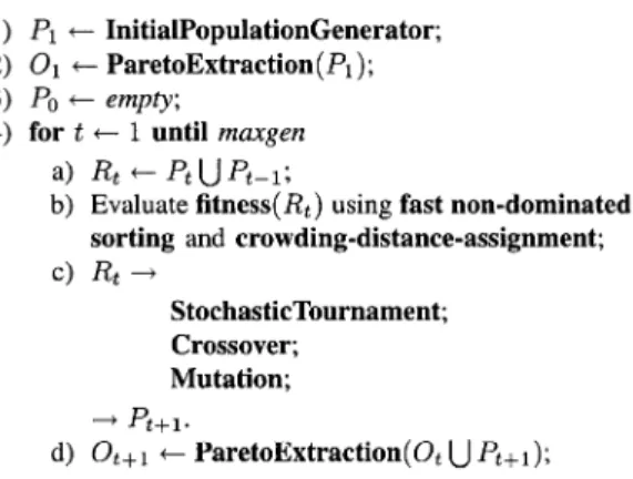
Fig. 2. Here, maxgen is the predefined number of generations to be executed. Each populationP hasN individuals (theStochasticTournamentoperator selects N individuals from its input of 2N individuals). The operator
ParetoExtractionreturns the nondominated set from the input set. The other operators are explained in the remainder of this section. The setO is the approximation of the Pareto set of the problem.
do not depend on the mono or multiobjective problem nature [22].
It should be noticed that a multiobjective GA evolves a whole population toward the Pareto set, instead of evolving a single “current point” to it. In a single run, the whole Pareto set or, at least, a large portion of this set will be found. This means that the ratio of the computational effort of executing a GA by the com-putational cost of executing a deterministic algorithm becomes much smaller in the case of multiobjective optimization prob-lems since a deterministic algorithm would have to run once a time for finding each Pareto point [3], [4].
V. PROBLEM-SPECIFICMULTIOBJECTIVEGA
The specific instance of multiobjective GA, which is used in this paper, is presented in this section. It is built on the basis of the selection and elitism operations of the NSGA-II algorithm [23]. Its structure is shown in Fig. 2.
The components of this algorithm are described in the fol-lowing subsections.
A. Selection and Elitism
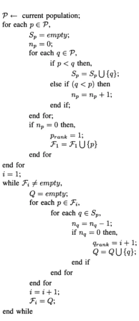
The selection operator is based on the nondominated sorting scheme [24], [25], using its optimized version, the fast-nondom-inated sorting [23], whose structure is shown in Fig. 3. This al-gorithm stores the results of each dominance comparison that has been performed in its first loop, in which the nondominated subset is determined. These data are used in the next loops for finding the next sets .
After the fast-nondominated sorting operation, the population
becomes separated in the subsets . Each subset
contains the individuals that are dominated by only those be-longing to the preceding sets, and the first set contains the individuals that are not dominated. This establishes a ranking in which the individuals of first frontier are in the best ranking position, and the individuals of the last one are in the worst position.
Fig. 3. Fast-nondominated sorting scheme of NSGA-2. The outputs of this procedure are the setsF.
The procedure of the crowding-distance-assignment process is described in Fig. 4. It estimates the density of solutions sur-rounding a particular solution in population [23]. This process, associated with the StochasticTournament, is a niche tech-nique, commonly employed in GAs. However, it has an advan-tage in relation to traditional niche methods, since it does not require any external parameters.
The selection operation of StochasticTournament makes the choice of individuals with the following procedure being re-peated times.
1) Two individuals and are chosen randomly.
2) The individual in the best position in the domination ranking (belonging to the set with smaller index ) is selected.
3) If and belong to the same set , then the individual with the greatest crowding value is selected. The NSGA-II is an elitist algorithm by its own structure: no additional operations are needed to introduce elitism.
With these selection and elitism operators, a GA becomes a “true multiobjective optimizer.” The entire Pareto set can be found with such an algorithm [4], [24], [25].
Fig. 4. Here,lis the number of individuals in the population.Iis the matrix with objective function values (vector of objectives of each individual, which are concatenated). The functionsort(I; m)sorts I by themth objective and I[i] 1 mreturns the value of objectivemof individuali.I[i] is the crowding value of individuali.
Fig. 5 Integer-variable encoding versus the traditional binary encoding.
B. Controlled-Greedy Encoding
The variables and the network structure of the problem ana-lyzed here suggest an encoding in which each part of the genetic word (usually called gene) represents one of the possible con-nections between nodes.
The genes could be represented by binary strings, as in tradi-tional GAs. However, this kind of representation generates large chromosomes, which is not so convenient. A more economic en-coding is employed here, which uses integer numbers to repre-sent the network connections of different possible types. Fig. 5 shows a comparison between the binary and the integer codifi-cation for a sample network. A second genetic word is used to represent the substations.
It must be of concern here of the fact that the number of problem variables (the possible connections between nodes) grows combinatorily, as the number of nodes grows. A naive encoding, allowing all possible connections between nodes, would constrain the GA to deal with very small networks only. The issue of explosive growing of problem dimensionality in combinatorial problems is dealt, in some heuristic methods for linear problems, by the so-called greedy algorithms [26]. In a given stage of building a network, for instance, these algo-rithms would try to put a connection that is the “best one” under the viewpoint of immediate cost, disregarding the fact that the globally cost-minimizing solution probably has some connec-tions that are not immediate minimizers.
Here, instead of performing such a deterministic short-term optimization procedure, the idea is to predefine the set of possible connections that a node could establish with other nodes. This set of allowed connections should be considered as optimization variables: only such connections are encoded, appearing in the search space of the algorithm. This is a kind of greedy procedure in the sense that several combinations are simply disregarded without being even evaluated, and only the seemingly reasonable ones are considered. In the case of electric networks, this procedure seems to be sensible since, in
real cases, a direct connection of too distant nodes would never occur. Only a set of neighboring nodes should be considered as alternatives for linking to a given node. This procedure has been used in most of the references that deal with the design of electric distribution networks, with the set of possible connec-tions for each node being established manually by the user. In this way, a smaller search space than the original one is defined. Here, an automatic procedure, called the controlled-greedy encoding, is proposed for establishing the set of possible con-nections. Two control parameters, which define the extent in which the search space is reduced, are required:
mxm maximum number of connection possibilities to be as-signed to any node;
mnn minimum number of connection possibilities to be as-signed to any node.
In the first step, the distance between all nodes is measured, and each node is assigned the mean distance between it and the other ones. The nodes are classified by their mean distances in ascending order. The node with minimum mean distance can connect to the mxn nearest nodes and the node with maximum mean distance can connect only to the mnn nearest neighbors. The number of connection possibilities (between mnn and mxn) for the other nodes is defined by a linear interpolation (according to the node mean distance) followed by a rounding operation.
(The actual set of connection possibilities which is encoded starts to be defined from the node with the smallest medium distance (which can connect to mxn nodes) to the node with maximum medium distance (which can connect to mnn nodes) including, in each step, the nearest connection alternatives, up to the number of connection possibilities that are assigned to each node.
For the 21-bus system that will be considered in the case study
section, in which and , the number of
vari-ables is reduced from 208 to 62. For the 100-bus system,
con-sidering and , the number of variables is
reduced from 4950 to 397.
After performing the controlled-greedy procedure, the set of impossible connections is considered. Some nodes that cannot be connected, due to geographical features, such as mountains, rivers, and other obstacles, are also excluded from the encoding. C. Initial Population
In classical GA algorithms, the initial population is randomly generated. However, for network problems with graph structure constraints, this procedure is not that efficient, because most of the random initial solutions do not represent feasible ones.
A classical graph algorithm has been employed here for dealing with this kind of network: the Prune algorithm, or inverse Kruskal algorithm [27]. For generating an individual of the initial population, a random initial network (that is connected and not radial) is generated, and its branches are placed in a list in descending order of costs, based on distances between nodes. The branches of are deleted from until they reach a feasible radial network. Then, the type of each conductor is assigned randomly. The procedure starts from different random initial networks and leads to networks that are different enough for providing a diversity of topologies
in the initial population3. However, all such solutions are based
on greedy operations. Therefore, they lack a diversity that is necessary for the GA to perform a global search.
This limitation is solved using a random network generator. This algorithm generates random networks that represent fea-sible and radial solutions. Most of the networks produced in this way have low quality, under both the objective function mea-sures, but they provide the necessary diversity of local config-urations that will be used, in the genetic operations, for finding globally optimizing networks.
After experimentation, it has been found that an equilibrium among the effects of the two procedures can be reached using the following composition of the initial population:
• 40% of individuals generated by Prune;
• 60% of individuals generated by the random network gen-erator.
D. Mutation and Crossover Operators
The classical GA operators that randomly change the individ-uals are not efficient in the problem considered here since, most of the time, they transform feasible solutions in infeasible ones (this is due to the graph-structure constraint). In few generations, the population becomes composed just of infeasible solutions. The following problem-specific operators have been built here to avoid this problem, leading to feasible solutions.
• Four crossover operators that determine the common part of two parent networks and copy this to the two children networks using the maximum or minimum indexes (de-pending on the operator). The way that the children will be completed will be different in each operator.
• Nine mutation operators that are divided into two classes: four of them consist of simple alterations in the type of branches or substations, which try a solution im-provement. They are named simple operators. The five remaining ones are based on some heuristics for changing the network topology. They are named smart operators. • Two named deterministic mutation operators are
em-ployed in order to improve the objective functions of the best cost network and of the best reliability network, with some deterministic operations. These operators are called deterministically (without a probabilistic call) each generations.
If the algorithm determines that a mutation or crossover must occur (depending on the crossover and mutation probabilities), an operator is chosen randomly with equal probability of each operator being used. This means that mutations that change the network topology occur in of mutation operator calls, and mutations that change the types of the network branches occur in of mutation operator calls.
A more detailed description of these 15 operators is given in Appendices A and B.
VI. NUMERICALRESULTS ANDANALYSIS
The proposed GA has been executed in the tests described here with the following parameters:
3At least one individual is always generated from the initial network which
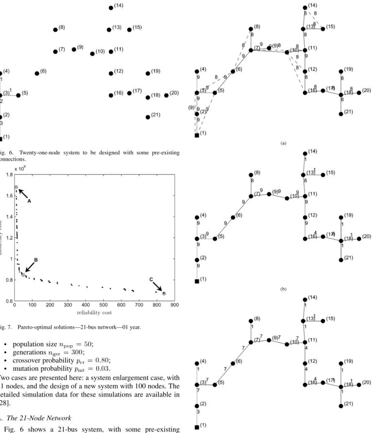
Fig. 6. Twenty-one-node system to be designed with some pre-existing connections.
Fig. 7. Pareto-optimal solutions—21-bus network—01 year.
• population size ;
• generations ;
• crossover probability ;
• mutation probability .
Two cases are presented here: a system enlargement case, with 21 nodes, and the design of a new system with 100 nodes. The detailed simulation data for these simulations are available in [28].
A. The 21-Node Network
Fig. 6 shows a 21-bus system, with some pre-existing connections that lead the GA to consider some “replacement costs” instead of “installation costs” in these locations. The controlled-greedy encoding has been used, considering the minimum number of connection possibilities for each node equal to 4 and the maximum number equal to 6. This results in a problem with 62 variables (possible connections). The results for this 21-bus system are presented for a one-year time range. The GA has found 137 Pareto optimal solutions as shown in Fig. 7. The network A is the most reliable network, and is
Fig. 8. Marked networks—21-bus network—01 year. The broken lines in Network A represent the reserve branches that have been used for enhancing system reliability. (a) Network A is the most reliable solution. (b) Network B is a balanced solution. (c) Network C is the smaller cost solution.
shown in Fig. 8(a). It should be noticed that up to seven reserve branches have been allowed: they have been used in Network A, for enhancing system reliability. The network C [Fig. 8(c)]
Fig. 9. One-hundred–node network—01 year. Network A is a balanced solution.
is the network with minimum cost and network B represents an intermediate solution that is probably better than both A and C, under the designer viewpoint. It should be noticed that B has a financial cost of , that is only 26.4% greater than the minimal cost network C, and is 50.4% smaller than the cost of the maximal reliability network A. The failure cost of B, that is 48.06, is 523.4% greater than that of network A, and is 94.3% smaller than that of network C. The networks A and B had all of the conductors of the pre-existing branches replaced by other ones with enhanced reliability. Network C had only two pre-existing conductors also replaced by other ones with smaller losses.
B. The 100-Node Network
Fig. 9 shows a 100-bus system which is a solution that has been found by the GA, considering one year as the time horizon for computing losses, and no pre-existing connections. The con-trolled-greedy encoding has been used, considering the min-imum number of connection possibilities for each node equal to 6 and the maximum number equal to 8. This results in a problem with 397 variables (possible connections).
The GA has found 132 Pareto-optimal solutions as shown in Fig. 10. The network of Fig. 9 corresponds to the solution marked with A in Fig. 10, which represents a balanced solution.
VII. DECISIONMAKINGWITH THEPARETOSET After obtaining the Pareto set, the designer has to choose which solution should be implemented: this is called the deci-sion-making process [18]. Some features of the decision process that are peculiar to the distribution network design problem are pointed out here.
First, it should be noted that the two objectives (financial cost and failure cost) are not independent: system faults lead to some financial penalty. Although the objective function (5) that rep-resents the system failure costs does not measure this financial
Fig. 10. Pareto-optimal solutions—100-bus network—01 year.
penalty, it can approximate this penalty. This can be accom-plished by a simple suitable scaling
(6) After this operation, the new objective function becomes expressed in monetary units, representing the monetary cost of system faults. In this scaling, a new cost function that aggre-gates all monetary costs can be defined (considering a given time horizon)
(7) This former cost is an approximation of the total monetary costs, including the installation cost, the energy losses, and the system fault penalties. There is, then, a minimal total monetary cost solution that minimizes the objective function . The entire Pareto set of the problem, that has been calculated in the space of the objectives , can be mapped to a new space, in the objectives , which, in fact, represents the tradeoff between reliability and financial cost. Several solutions, which belong to the initial Pareto set, become dominated in the new space, and the minimal total monetary cost solution becomes an
Fig. 11. The original Pareto set in spacef 2 f , with the solutions I to V, and the mapping of these solutions to the new spacef 2 f . All solutions keep the same failure indexf in both spaces and have the total monetary costf greater than the initial monetary costf . Solutions I and II become dominated in this new space. Solution III is the minimal total monetary cost one.
Fig. 12. The marginal cost of changing from the solution I to solution II = is different from the cost of changing from solution II to solution III = and so forth. Each solution change involves its own marginal cost associated to the added reliability.
extremal solution of the new (transformed) Pareto set, situated in an end of this set. This operation is represented in Fig. 11.
The final choice of the solution for implementation purpose should finally be performed according to the regulatory context: i) In a “savage monopoly” context, the monopolistic company would simply choose the solution that minimizes . ii) In a regulated market, the regulatory agency and the electric utility company can discuss the solution to be adopted in the context of an energy pricing policy. The marginal monetary cost of increasing the system reliability, when going from solution to solution can be clearly identified in the transformed Pareto set , as shown in Fig. 12. This information allows the public policy maker for deciding what reliability index should be attained, knowing which would be its cost. This decision can be different for different system nodes (this is the role of the “im-portance index” which is adopted in (5)). Notice that the mar-ginal cost in the change of any solution varies along the Pareto set solutions, as shown in Fig. 12, and this information is to be extracted from the Pareto set graphics. iii) Finally, in a com-petitive market, both energy selling cost and energy reliability index would influence the market equilibrium among competi-tors. The information of the transformed Pareto set
brings to the company managers the possibility of performing a quantitative technical analysis when taking a decision related to energy pricing and network installation investment.
VIII. CONCLUSION
This paper has presented a multiobjective approach for the design of electric distribution networks that considers the objec-tives of minimizing the overall monetary costs and minimizing a system failure index. A multiobjective GA, using problem-spe-cific mutation and crossover operators and an efficient variable encoding scheme, has been employed as the optimization ma-chinery for finding the Pareto-optimal solutions. Both cases of the design of new networks and the design of expansion in ex-isting networks are addressed by the proposed algorithm.
The information provided by the Pareto-optimal set has been shown to be more valuable for the purpose of aiding the decision on the investment policy to be adopted by the energy companies than the traditional mono-objective optimal solutions that the former approaches are able to find.
APPENDIX A CROSSOVEROPERATORS A. SmartXOver1—Crossover Operator
1) Two networks ( and ) are selected in population. The common branches are identified in these networks
. Two graphs are created with the remaining branches
( and ).
2) The common branches are copied to the children net-works using the conductors with maximum capacity
( and ).
3) If represents an infeasible solution, the branches of are copied to in costs descending order. This process repeats until it represents a feasible solution. So the re-serving branches of are copied to .
4) The same process is applied to , using the branches of .
B. SmartXOver2—Crossover Operator
It is similar to SmartXOver1 (topic I.A) but in item 2, the conductors’ minimum capacity is used to compose and
( and ).
C. SmartmiXOver1—Crossover Operator
1) Two networks ( and ) are selected in population. The common branches are identified in these networks
. Two graphs are created with the remaining branches
( and ).
2) The common branches are copied to the children networks being created with the conductors of minimum capacity
( and created with the branches of
maximum capacity ).
3) All branches of and are copied to and . 4) In the last step, and are radialized, cutting the
branches with maximum length. D. SmartmiXOver2—Crossover Operator
1) It is similar to SmatMixOver1, differing only in the last step, where in the branches with maximum index are cut and in the branches with minimum index are cut until they become radial networks.
APPENDIX B MUTATIONOPERATORS A. SmartMutation1—Mutation Operator
1) The parent network is copied to the child network . 2) A graph is created with all possible branches
. The complementary graph of is .
3) The branches of are ordered in descending order of fixed costs (based on distance between nodes) in a vector
.
4) The first branch of is selected and inserted in . Source and destination nodes of the selected branch are identified.
5) All branches connected to and in are evaluated and the most expensive branch is deleted.
6) The radiality and feasibility constraints are checked in the resulting network. If one of them or both have been vi-olated, the deleted branch in 5 is inserted, the inserted branch in is deleted, and the next branch of is chosen. B. SmartMutation2—Mutation Operator
1) The parent network is copied to the child network . 2) A graph is created with all possible branches
. The complementary graph of is .
3) The branches of are ordered in ascending order of fixed costs (based on distance between nodes) in a vector . 4) The first branch of is selected and deleted from .
Source and destination nodes of the selected branch are identified.
5) All branches connected to and in network are evaluated. The branch with smaller cost is inserted in . 6) The radiality and feasibility constraints are checked in the resulting network. If one of them or both have been violated, the inserted branch in 5 is deleted, the deleted branch in 4 is inserted, and the next branch of is chosen. C. SmartMutation3—Mutation Operator
1) A network is selected and copied to the child network .
2) If any node has more than one reserve branch, the larger reserve branch is deleted.
D. SmartMutation4—Mutation Operator
1) A network is selected and copied to the child network .
2) The nodes are ordered in ascending order of importance in a vector .
3) The first node of is selected. If it does not have any reserve branches, then a reserve branch is created. Else, the next node of is selected.
E. SmartMutation5—Mutation Operator
1) A network is selected and copied to the child network .
2) If a node does not have any alternative supply source in any branch failure, then a reserve branch is created in this node.
F. SimpleMutation1—Mutation Operator
1) A network is selected and copied to the child network .
2) A conductor is chosen randomly.
3) The conductor with maximum capacity of is chosen
and if , then is changed by .
G. SimpleMutation2—Mutation Operator
1) A network is selected and copied to the child network .
2) A substation is chosen randomly.
3) The substation with maximum capacity of is chosen
and if , then is changed by .
H. SimpleMutation3—Mutation Operator
1) A network is selected and copied to the child network .
2) The branch with larger failure rate is selected. 3) A conductor is chosen randomly.
4) If has a smaller failure rate, then is replaced by . I. SimpleMutation4—Mutation Operator
1) A network is selected and copied to the child network ;
2) The power flow of is calculated and the conductors of are replaced by those with minimum acceptable ca-pacity.
J. DeterministicMutation1—Cost Improvement
1) At each generations, the network with minimum cost is determined and copied to .
2) Each branch of is replaced by one with an optimal index. The network layout (topology) is not changed. 3) If the resulting network has a cost that is lower than
cost, then replaces .
K. DeterministicMutation2—Reliability Improvement
1) At each generations, the minimum cost network is determined and copied to .
2) Each branch of is replaced by one with a lower failure rate. The network layout (topology) is not changed. 3) If the resulting network is more reliable than , then
replaces .
REFERENCES
[1] J. L. Verwers and J. R. Sovers, “Challenges of supplying electric power to a large industrial customer in rural areas,”IEEE Trans. Ind. Appl., vol. 36, no. 4, pp. 972–977, Jul./Aug. 2000.
[2] S. Ching-Tzong and L. Guor-Rurng, “Reliability design of distribution systems using modified genetic algorithms,”Elect. Power Syst. Res., vol. 60, pp. 201–206, 2002.
[3] C. M. Fonseca and P. Fleming, “An overview of evolutionary algorithms in multiobjective optimization,”Evol. Comput., vol. 3, no. 1, pp. 1–16, 1995.
[4] C. A. C. Coello, “An updated survey of GA-based multiobjective opti-mization techniques,” inProc. ACM Computing Surveys, vol. 32, 2000, pp. 109–143.
[5] S. Pierre, “Application of artificial intelligence techniques to computer network design,”Eng. Appl. Artif. Intell., vol. 6, no. 5, pp. 465–472, 1993.
[6] D. K. Smith and G. A. Walters, “An evolutionary approach for finding optimal trees in undirected networks,”Eur. J. Oper. Res., vol. 120, pp. 593–602, 2000.
[7] F. R. B. Cruz, M. G. Smith, and G. R. Mateus, “Solving to optimality the uncapacitated fixed-charge network flow problem,”Comput. Oper. Res., vol. 25, no. 1, pp. 67–81, 1998.
[8] G. Duan and Y. Yu, “Power distribution system optimization by an algo-rithm for capacitated Steiner tree problems with complex-flows and ar-bitrary cost functions,”Elect. Power Energy Syst., vol. 25, pp. 515–523, 2003.
[9] V. Miranda, J. V. Ranito, and L. M. Proença, “Genetic algorithms in optimal multistage distribution network planning,”IEEE Trans. Power Syst., vol. 9, no. 4, pp. 1927–1933, Nov. 1994.
[10] I. Ramírez-Rosado and J. Bernal-Agustín, “Genetic algorithms applied to the design of large power distribution systems,”IEEE Trans. Power Syst., vol. 13, no. 3, pp. 696–702, Aug. 1998.
[11] J. L. Bernal-Agustín, “Aplicación de algoritmos genéticos al diseño óp-timo de sistemas de distribución de energía eléctrica,” Ph.D. dissertation, Zaragoza Univ., Zaragoza, Spain, 1998.
[12] P. M. S. Carvalho, L. Ferreira, F. Lobo, and L. Barruncho, “Optimal dis-tribution network expansion planning under uncertainty by evolutionary decision convergence,”Elect. Power Energy Syst., vol. 20, no. 2, pp. 125–129, 1998.
[13] D. Das, “Reactive power compensation for radial distribution networks using genetic algorithm,” Elect. Power Energy Syst., vol. 24, pp. 573–581, 2002.
[14] G. Duan and Y. Yu, “Problem-specific genetic algorithm for power trans-mission system planning,”Elect. Power Syst. Res., vol. 61, pp. 41–50, 2002.
[15] J. Z. Zhu, “Optimal reconfiguration of electrical distribution network using the refined genetic algorithm,”Elect. Power Syst. Res., vol. 62, pp. 37–42, 2002.
[16] J. F. Goméz, H. M. Khodr, P. M. de Oliveira, L. Ocque, J. M. Yusta, R. Villasana, and A. J. Urdaneta, “Ant colony system algorithm for the planning of primary distribution circuits,”IEEE Trans. Power Syst., vol. 19, no. 2, pp. 996–1004, May 2004.
[17] A. Cossi, R. Romero, and J. Mantovani, “Planning of secondary distribu-tion circuits through evoludistribu-tionary algorithms,”IEEE Trans. Power Del., vol. 20, no. 1, pp. 205–213, Jan. 2005.
[18] V. Chankong and Y. Y. Haimes,Multiobjective Decision Making: Theory and Methodology. Amsterdam, The Netherlands: Elsevier, 1983. [19] H. L. Willis, H. Trans, and L. F. M. V. Engel, “Selecting and applying
distribution optimization methods,”IEEE Comput. Appl. Power, vol. 9, no. 1, pp. 12–17, Jan. 1996.
[20] Y. Tang, “Power distribution system planning with reliability modeling and optimization,”IEEE Trans. Power Syst., vol. 11, no. 1, pp. 181–189, Feb. 1996.
[21] R. H. C. Takahashi, J. A. Vasconcelos, J. A. Ramirez, and L. Krahenbuhl, “A multiobjective methodology for evaluating genetic operators,”IEEE Trans. Magn., pt. 1, vol. 39, no. 3, pp. 1321–1324, May 2003. [22] R. H. C. Takahashi, R. M. Palhares, D. A. Dutra, and L. P. S. Gonçalves,
“Estimation of pareto sets in the mixedH =H control problem,”Int. J. Syst. Sci., vol. 35, pp. 55–67, 2004.
[23] K. Deb, A. Pratap, S. Agrawal, and T. Meyarivan, “A fast and elitist mul-tiobjective genetic algorithm: NSGA-II,”IEEE Trans. Evol. Comput., vol. 6, no. 2, pp. 182–197, Apr. 2002.
[24] N. Srinivas and K. Deb, “Multiobjective optimization using nondomi-nated sorting in genetic algorithms,”Evol. Comput., vol. 2, no. 3, pp. 221–248, 1994.
[25] A. Augugliaro, L. Dusonchet, and E. R. Sanseverino, “Evolving non-dominated solutions in multiobjective service restoration for automated distribution networks,”Elect. Power Syst. Res., vol. 59, pp. 185–195, 2001.
[26] U. K. Sarkar, P. P. Chakrabarti, S. Ghose, and S. C. DeSarkar, “Im-proving greedy algorithms by lookahead search,”J. Algorithms, vol. 16, pp. 1–23, 1994.
[27] M. S. Bazaraa and J. J. Jarvis, Linear Programming and Network Flows. New York: Wiley, 1977.
[28] E. G. Carrano, R. H. C. Takahashi, E. P. Cardoso, O. M. Neto, and R. R. Saldanha, “Multiobjective genetic algorithm in the design of electric distribution networks: simulation data,” Univ. Fed. Minas Gerais, http://www.mat.ufmg.br/~taka/techrep/agnet01.pdf, Tech. Rep., 2005. available in.
Eduardo G. Carranowas born in Divinópolis, Brazil, in 1981. He received the B.Sc. degree in electrical engineering from Universidade Federal de São João Del Rei in 2003. He is currently pursuing the Ph.D. degree from the Universi-dade Federal de Minas Gerais, Belo Horizonte, Brazil.
His research interests include network optimization, multiobjective optimiza-tion, stochastic and deterministic optimization algorithms, neural networks, and fuzzy systems.
Luis A. E. Soareswas born in Belo Horizonte, Brazil, in 1963. He received the B.Sc. and M.Sc. degrees in electrical engineering from Universidade Federal de Minas Gerais in 1985 and 2001, respectively.
Currently, he is a Senior Consulting Engineer with Strike Engenharia, Belo Horizonte, Brazil, where he develops power systems studies and electrical system design for industrial facilities.
Ricardo H. C. Takahashiwas born in Ipatinga, Brazil, in 1965. He received the B.Sc. and M.Sc. degrees in electrical engineering from Universidade Federal de Minas Gerais (UFMG), Belo Horizonte, Brazil, in 1989 and 1991, respectively, and the Ph.D. degree in electrical engineering from the University of Campinas, Campinas, Brazil, in 1998.
Currently, he is with the Department of Mathematics, UFMG, where he has been since 2002. He was with the Department of Electrical Engineering at UFMG from 1992 to 2002. His research interests are optimization theory and control theory.
Rodney R. Saldanhawas born in Belo Horizonte, Brazil, in 1954. He received the B.Sc. degree in electrical engineering from the Universidade Federal de Minas Gerais (UFMG), Belo Horizonte, Brazil, in 1980, the M.Sc. degree in electrical engineering from UFMG in 1983, and the Ph.D. degree in electrical engineering from the Institut National Polytechnique de Grenoble, Grenoble, France, in 1992.
Currently, he is with the Department of Electrical Engineering, UFMG. His research interests are in the design and optimization of electromagnetic devices.
Oriane M. Netowas born in Brazil in 1961. He received the B.Sc. and M.Sc. degrees in electrical engineering from Universidade Federal de Minas Gerais (UFMG), Belo Horizonte, Brazil, in 1985 and 1989, respectively, and the Ph.D. degree from Imperial College of Science, Technology and Medicine, London, U.K., in 1996.
Currently, he is with the Department of Electrical Engineering, UFMG. He was a Visiting Professor with the Department of Electrical Engineering, Tokyo Metropolitan University, Tokyo, Japan, from 2001 to 2002. His research inter-ests are in power system dynamics and power system optimization and control.