Multiple prediction through inversion: Theoretical advancements and real data application

(1)

Multiple prediction through inversion: Theoretical advancements

and real data application

Yanghua Wang

1

ABSTRACT

Wave-equation-based multiple attenuation seismic meth-ods may be divided into the two distinct phases of multiple modeling and multiple subtraction. These two are interrelat-ed and must be optimizinterrelat-ed in order to produce an optimal final result. The multiple prediction through inversion 共MPI兲 scheme updates the multiple model iteratively, as we usually do in a linearized inverse problem. The scheme models the multiple wavefield without an explicit knowledge of surface and subsurface structures or of the source signature; both are generally unknown in seismic surveys. However, compared to a conventional surface-related multiple attenuation meth-od, the accuracy of the multiple model is improved both kine-matically and dynamically. It is because the MPI scheme im-plicitly takes account of the spatial variation of the surface flectivity, the source signature, the detector patterns and re-ceiver ghosts, and other effects included in the so-called surface operator. When the MPI scheme is used in the first phase it also significantly reduces the nonlinearity of the problem in the second phase that involves attenuating multi-ples without removing or altering primaries. The effective-ness of the MPI scheme is demonstrated by examples involv-ing real marine seismic data.

INTRODUCTION

The attenuation of multiple reflections in surface seismic data has been a high priority in research and development in both operating and service companies for many years. Many partial solutions exist that are able to ameliorate the problem in specific circumstances. This is particularly the case for marine seismic data. There is, how-ever, no method or group of methods that works in all cases; in many cases, multiple contamination is still the controlling limit on noise

and resolution. This is true for surface-related multiples on land seis-mic data and for interbed multiples on all data.

Among various multiple attenuation techniques, a suite of free-surface multiple attenuation共SMA兲 methods has been developed that seeks to predict the multiple wavefield directly from the seismic field data. These methods use minimal assumptions about the struc-ture of the subsurface and then seek to subtract this共imperfect兲 pre-diction from the field data in some optimum manner共Verschuur et al., 1992; Verschuur and Berkhout, 1997; Weglein et al., 1997; Dragoset and Jeriçevíc, 1998; Luo et al., 2003; Guitton, 2005兲. In many circumstances, particularly those involving moderately two-dimensional structures on marine data without strong interbed mul-tiples共as conventional SMA methods treat the interbeds as prima-ries兲, these methods work well共Hadidi et al., 2002兲. On many other data sets, especially those acquired on land共Kelamis and Verschuur, 2000兲, those that are monotonously one-dimensional with strong in-terbed multiples, and those that are highly three-dimensional, exist-ing multiple-suppression methods are often inadequate共Baumstein et al., 2005兲. This is particularly important when the utility of the in-terpretation requires maximum spatial resolution of weak primaries or depends upon the interpretation of subtle characteristics of the data extracted prestack.

For SMA methods, the multiple attenuation procedure may be di-vided into the two distinct phases of multiple prediction and multiple subtraction. These two parts are interrelated, and both must be opti-mized in order to produce an optimal final result. Wang共2003a, 2004兲has proposed two complementary, novel, and promising con-cepts for multiple attenuation:共1兲multiple prediction through inver-sion for multiple modeling and共2兲expanded multichannel matching for multiple subtraction. These yield both improved prediction and improved subtraction. Together they appear to overcome some of the limitations of the previously mentioned existing methods.

The core of this series of multiple attenuation techniques is the multiple prediction through inversion共MPI兲concept for modeling the multiple wavefield. The MPI scheme refines the multiple model through iteration, just as we usually do in an iterative inverse prob-lem. Further, I offer two theoretical justifications of the MPI con-Manuscript received by the Editor February 12, 2006; revised manuscript received August 29, 2006; published online January 11, 2007.

1_{Imperial College London, Department of Earth Science and Engineering, Centre for Reservoir Geophysics, London, United Kingdom. E-mail: yanghua.wang} @imperial.ac.uk.

V33

(2)

cept. First, consider the multiple attenuation as an optimization problem. For each iteration, the cost function is optimized from one level to the next by updating the current model共wavefield兲. A de-sired updating direction should be normal to the next level共contour兲 of the cost function. In the MPI concept, searching for the desired updating direction can be implemented in two steps:共1兲setting a preliminary updating direction that emits normally from the current level共contour兲of the cost function and共2兲then adjusting the tion by a proper adaptive subtraction, so that the final updating direc-tion has a normal incident angle impinging at the next level共contour兲 of the cost function.

The second theoretical justification is that the MPI scheme takes into account the surface operator implicit in multiple modeling. The surface operator consists of effective source characteristics, reflec-tivity of the multiple-generating interface, and many other effects

共Berkhout, 1982, 1984兲. Almost all methods now in use require ex-plicit knowledge of these effects, which are problematic and highly variable spatially. Because the MPI scheme implicitly takes account of these effects, it generates a multiple model with both kinematical-ly and dynamicalkinematical-ly improved accuracy. It also significantkinematical-ly reduces the nonlinearity of the problem in the subsequent adaptive subtrac-tion phase.

MULTIPLE PREDICTION THROUGH INVERSION The MPI concept

This section provides an alternative but concise derivation to the MPI formula presented in Wang共2004兲for multiple modeling.

Consider the multiple attenuation problem as an optimization problem and denotePto represent the data set consisting of prima-ries and multiples andP0to represent the desired data set without any

multiples. The optimization is performed iteratively, andP0共 n兲_{is the}

multiple attenuation result after thenth iteration.

Suppose that after the共n− 1兲th iteration the multiple attenuation resultP₀共n−1兲_{is obtained from the previous iteration result}_P

0

共n−2兲_{; a}

convolution operatorT共n−1兲_{may be introduced to link} _P

0

共n−1兲 _and

P₀共n−2兲_:

P₀共n−1兲= T共n−1兲P₀共n−2兲. 共1兲 The updating operatorT共n−1兲_{can be estimated as}

T共n−1兲=P₀共n−1兲共P₀共n−2兲兲H关P₀共n−2兲共P₀共n−2兲兲H兴−1. 共2兲 ThisT共n−1兲_{operator is borrowed for the}_n_{th iteration to predict}_P

0 共n兲_, P ˜ 0 共n兲 =T共n−1兲P₀共n−1兲, 共3兲

whereP˜₀共n兲_{represents an approximation because}_T共n−1兲_{is estimated}

from the previous iteration result and is not the accurateToperator for the current iteration共T共n兲_兲_.

Equation 3 for primary prediction can easily be transferred to an equation for multiple prediction. Following Berkhout and Vers-chuur共1997兲, the free-surface multiple wavefieldMmay be defined as

M= P0AP, 共4兲

whereAis a so-called surface operator, physically a convolution of the inverse source signature, the free-surface reflectivity, effects of detector patterns and receiver ghosts, and many other effects

共Berkhout, 1982, 1984兲. Equation 4 may be used to rewrite equation 3 as M˜共n兲 =T共n−1兲M共n−1兲, 共5兲 whereM˜共n兲₌_P˜ 0 共n兲_AP_and_M共n−1兲₌_P 0 共n−1兲_AP_{. If equation 2 is}

substi-tuted into equation 5, the MPI formula is obtained as

M˜共n兲= P₀共n−1兲共P₀共n−2兲兲H关P₀共n−2兲共P₀共n−2兲兲H兴−1共P− P₀共n−1兲兲,

共6兲

fornⱖ2.

Once the multiple modelM˜共n兲_{is generated, an adaptive}

subtrac-tion scheme can be used to obtain the multiple attenuasubtrac-tion result as

P0共 n兲

=P− ⌳M˜共n兲, 共7兲

where⌳is the adaptive filter presented in the frequency domain, but commonly is estimated in the time domain as a multichannel shaping filter共Wang, 2003a兲. In an iterative multiple attenuation scheme, equations 6 and 7 are the two phases of modeling and subtraction that form one iteration.

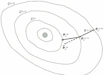
The justification for the use of theT共n−1兲_{operator is illustrated in}

Figure 1. The previous iteration has made the best effort to obtain a result共P0共n−1兲兲. The best effort means that vectorP0共n−2兲→P0共n−1兲is a

normal incident vector impinging onC共n−1兲_{, the contour of the cost}

function that is optimized locally. VectorP0共n−2兲→P0共n−1兲is theT共n−1兲

operator to which I refer. In the current iteration, the multiple model-ing phaseP˜₀共n兲₌_T共n−1兲_P

0

共n−1兲_{means that vector}_P

0

共n−1兲_→_P˜

0

共n兲_{has a}

nor-mal emitting angle emerging from the contourC共n−1兲_{, and the}

adap-tive subtraction phase means wavefield moderation fromP˜₀共n兲_to_P

0

共n兲_.

The latter determines the step length and also tunes the update direc-tion, so that a new vectorP₀共n−1兲_→_P

0

共n兲_共_{i.e., the}_T共n兲_operator_兲_finally

impinges on contourC共n兲_{with a normal incident angle.} P0(n) T(n–1) P0(n–1) P0(n–2) C(n–2) C(n–1) C(n) P0(n) ~

Figure 1. In the MPI scheme, the modeling phase is represented by vectorP₀共n−1兲_→_P˜

0

共n兲_{, which has a normal emitting angle emerging}

from the contourC共n−1兲_{, and the adaptive subtraction phase is}

repre-sented by vectorP˜0共

n兲_→_P

0

共n兲_{, which finally makes vector}_P

0

共n−1兲_→_P

0

共n兲

normal to the contourC共n兲_{. The}_T共n−1兲_{operator represents the}

previ-ous iterationP0共n−2兲→P0共n−1兲, which has a normal incident angle

im-pinging at the contourC共n−1兲_.

(3)

Improvements to conventional SMA

A conventional SMA assumes that the surface operatorAin equa-tion 4 is a scalar and predicts multiples by using the following spatial convolution共Verschuur and Berkhout, 1997兲:

M˜共n兲 ₌_P 0

共n−1兲_P_. _共₈_兲

Then an adaptive subtraction phase partially recovers the effect of the surface operatorAomitted in equation 8. The next iteration throws away this effort and again starts multiple modeling with the same assumption. By contrast, the effort made in the previous itera-tion for recovering the spatial variaitera-tion in the surface operatorAhas been kept in the MPI scheme.

The MPI scheme modifies the multiple wavefield obtained in the previous iteration to build a multiple model for a new iteration, as shown in equation 5. The MPI scheme can be understood as

M˜共n兲₌_P 0 共n−1兲_A共n−1兲_P_, _共₉_兲 and A共n−1兲⬇ 关P₀共n−2兲兴−1共P− P共₀n−1兲兲P−1⬇ 关P₀共n−1兲兴−1− P−1. 共10兲

Detailed derivation can be found in Wang共2004兲. Even though the A共n−1兲_{operator reconstructed from the previous iteration is not}

suffi-ciently accurate, including it in multiple modeling will improve the accuracy of the modeled multiple wavefieldM˜共n兲_{kinematically and}

dynamically, if compared with the conventional SMA in equation 8. Meanwhile, it significantly reduces the nonlinearity of the problem for the adaptive subtraction. In MPI, the surface operator is not ex-plicitly presented in multiple modeling, but is included imex-plicitly in equations 5 and 6.

MPI starts fromn= 2, for whichP₀共0兲_and_P

0

共1兲_{are needed for}

esti-mating the firstToperatorT共n−1兲₌_T共1兲_{. In practice,}_P

0

共0兲₌_P_{, the}

original data matrix, is often assumed. ForP₀共1兲_{, either a conventional}

SMA or moveout equation-based method共Wang, 2003a兲 can be used to model the multiple, followed by an adaptive subtraction. Other methods such as Radon-domain multiple attenuation共Wang, 2003b兲can also be used to obtainP₀共1兲_{directly. Although a}

conven-tional SMA method could be used to initiate the iteration, the central idea of the MPI scheme is that at each iteration the accuracy of multi-ple modeling is maximized, so that the subsequent subtraction can be optimized or linearized.

In MPI, an operatorTis used to modify the multiple wavefield ob-tained in the previous iteration. Within theToperator共equation 2兲, the calculation involves auto- and crosscorrelations of common-re-ceiver gathers, rather than the spatial convolution between shot gath-ers共equation 8兲used in a conventional SMA method. Because the MPI scheme is not formulated explicitly in terms of a spatial convo-lution, the scheme manages to minimize the edge effects that appear in a conventional SMA multiple prediction 共Wang, 2004兲. This leads to greater stability and accuracy and is of particular relevance to land acquisition, where the shooting geometry is often controlled by the terrain rather than by the requirements of a particular process-ing algorithm. Because of this property, the MPI scheme also elimi-nates the need to synthesize near-offset traces, required by a conven-tional SMA scheme, and so it can work for a seismic data set with missing or noisy near-offset traces共Wang, 2004兲.

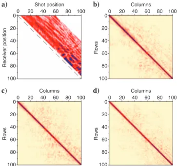
Figure 2a displays a data matrixPin the frequency domain. Each column represents a shot record, and each row a common-receiver

gather共Berkhout, 1982兲. Figure 2a shows the amplitude values of all traces for a single-frequency component. Note that the dashed line indicates the zero-offset position; in this example, five near-offset traces were missing. A conventional SMA method would require filling out the near offsets共i.e., the data around the main diagonal兲 and even some of the offsets at the other side of the diagonal. In the MPI method, theToperator is nearly a diagonal-band matrix, as shown in Figure 2b-d, theT共n−1兲_{operators for}_n_{= 2, 3, and 4,}

respec-tively. Equation 5 indicates that such a narrow-band diagonal matrix acts as complex-valued weighting on the multiple-wavefield matrix; therefore, there is no edge effect, and missing near-offset data does not affect theToperator.

TheToperator, calculated by using equation 2, is nearly a narrow-band matrix. Wang共2004兲suggests approximating theToperator as a tridiagonal matrix and then speeding up the computation signifi-cantly. In addition, theToperator converges to a diagonal matrix. Such convergence fromn= 3 ton= 4 is marginal共see Figure 2c and d兲; thus three iterations are usually sufficient for real data pro-cessing, as indicated by Wang共2004兲.

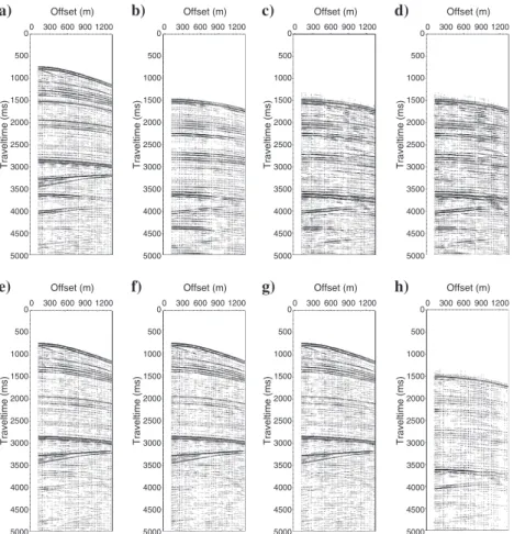
Figure 3a is a sample shot record, a column vector of data matrixP in the frequency domain. Figure 3b-d displays the predicted multiple model of the first, second, and third iterations, a column vector of M˜共1兲_,_M˜共2兲_{, and}_M˜共3兲_{, respectively. Figure 3e-g shows the multiple}

at-tenuated gather after the first, second, and third iterations, a column vector ofP0共1兲,P0共2兲, andP0共3兲, respectively. Note that the residuals att

= 1500 and 4000 ms at near offsets are suppressed through itera-tions. Figure 3h is the difference between Figure 3a and 3g共i.e., the multiple energy attenuated after the third iteration, a column vector ofM共3兲_{in the frequency domain}_兲_{. This shot-gather example is}

arbi-trarily selected from a synthetic data set, Pluto 1.5. Stacked sections before and after MPI multiple attenuation were shown in Wang

共2004兲.

b)

0 20 40 60 80 100 Columns Ro ws 20 0 40 60 80 100

a)

0 20 40 60 80 100 Shot position Receiv er position 20 0 40 60 80 100

d)

0 20 40 60 80 100 Columns Ro ws 20 0 40 60 80 100

c)

0 20 40 60 80 100 Columns Ro ws 20 0 40 60 80 100

Figure 2.共a兲A data matrix in which each column represents a shot record in the frequency domain and each row is a common receiver gather. In this example, five near-offset traces are missing, and a di-agonal line indicates the zero-offset positions.共b–d兲TheT共n−1兲

oper-ators forn= 2, 3, and 4, respectively.

(4)

REAL DATA EXAMPLES

This section demonstrates the effectiveness of the MPI scheme by using two real data examples from marine seismic surveys. In the first real data set, the original shot interval is 50 m, four times the ceiver interval, which is 12.5 m. In practice, an SMA technique re-quires a shot at every receiver station. Shot interpolation is per-formed by using the f-x-y domain trace-interpolation method

共Wang, 2002兲, wherefis the frequency andxandyare the two spa-tial axes representing the shot location and the source-receiver off-set, respectively. Thef-x-ydomain trace-interpolation method can relax the requirement that events must be linear in anf-xdomain method. Events that are nonlinear in one direction but linear in an-other may be interpolated exactly with anf-x-yinterpolation filter.

Figure 4a displays a sample shot gather, consisting of 14 missing near-offset traces共the offset between 0 and 162.5 m兲and 48 live traces共the offset between 175 and 762.5 m兲. Figure 4b and c shows a multiple attenuation gather and the attenuated multiple energy. Gathers in the zoomed-in version in Figure 4 show clearly that over-lapping primaries and multiples can be well separated in this pro-cessing.

It is worthwhile to point out that although MPI provides an accu-rate multiple prediction, the effectiveness of multiple attenuation de-pends upon the adaptive subtraction scheme adopted. Here, we use the expanded multichannel matching method共Wang, 2003a兲. For a

normal multichannel matching, where an original seismic trace is matched by a group of multiple-prediction traces, the lateral coher-ency of adjacent traces is typically exploited to discriminate between overlapping multiple and primary reflections. In the expanded multi-channel matching, a seismic trace is matched not only by a group of predicted multiple traces, but also by a number of mathematically re-lated traces. If the convolution coefficients associated with the nor-mal multichannel filter are presented as a 2D operator in the time-space domain, this 2D operator is now expanded with an additional spatial dimension to improve the robustness of the adaptive subtrac-tion.

In the expanded multichannel matching, the mathematically relat-ed traces include the first derivatives, the Hilbert transforms, and the first derivatives of their Hilbert transforms. Differentiation with re-spect to time is equivalent to multiplication by frequency in the fre-quency domain. Because multiplication by frefre-quency enhances higher relative to lower frequencies, it can sometimes change the ap-pearance of a seismic trace dramatically. Therefore, use of the ex-panded traces will improve the matching resolution in time.

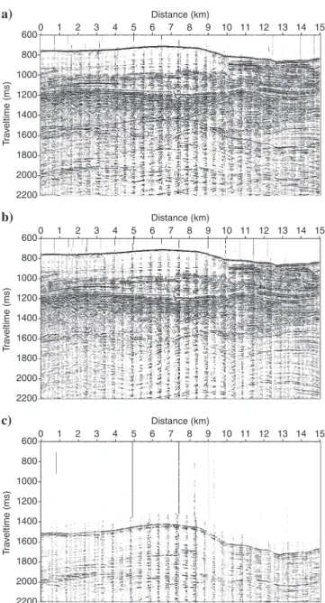
Figure 5a is the stack section of the first real data set, which shows a complicated structure under the water bottom. The water depth is about 525–675 m共700–900 ms in two-way traveltime兲. Figure 5b presents the stack section after multiple attenuation, and Figure 5c displays the attenuated multiple energy. On close examination of the multiple attenuation result between 1500 and 2100 ms, it can be seen that the spatial structure of weak reflections with lateral continuation has been revealed. Free-sur-face multiples have been cleanly attenuated, without removing the primary. The three sections in Figure 5 are plotted by using the same ampli-tude scale.

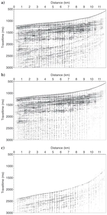
Figure 6 shows another real data example. Each shot gather consists of 100 channels with 12.5-m intervals; the shot spacing is 25 m. Thef

-x-ytrace interpolation is used again to generate a new shot gather between a pair of shots. This makes the final shot interval 12.5 m, the same as the receiver interval. Figure 6a shows the brute stack before multiple attenuation, Figure 6b dis-plays the multiple attenuation result using the MPI scheme presented in this paper, and Figure 6c illustrates the energy removed by MPI关i.e., the difference between the original stack section

共Figure 6a兲 and the multiple attenuation result

共Figure 6b兲兴.

DISCUSSION

Examples have demonstrated that the MPI scheme can work for seismic data with missing near-offset traces. This is one of the advantages compared to conventional SMA methods. For marine seismic reflection data, if the source sig-nature and the near-surface reflectivity can be as-sumed to be approximately constant, another dif-ference between MPI and conventional SMA methods is that MPI effectively includes deghost-ing, whereas SMA does not. A conventional SMA needs a proper deghosting prior to multiple modeling共Verschuur et al., 1992兲. For a

deghost-b) 0 500 1000 1500 2000 2500 3000 3500 4000 4500 5000 Offset (m) Traveltime (ms) 300 0 600 900 1200 a) 0 500 1000 1500 2000 2500 3000 3500 4000 4500 5000 Offset (m) Traveltime (ms) 300 0 600 900 1200 d) 0 500 1000 1500 2000 2500 3000 3500 4000 4500 5000 Offset (m) Traveltime (ms) 300 0 600 900 1200 c) 0 500 1000 1500 2000 2500 3000 3500 4000 4500 5000 Offset (m) Traveltime (ms) 300 0 600 900 1200 f) 0 500 1000 1500 2000 2500 3000 3500 4000 4500 5000 Offset (m) Traveltime (ms) 300 0 600 900 1200 e) 0 500 1000 1500 2000 2500 3000 3500 4000 4500 5000 Offset (m) Traveltime (ms) 300 0 600 900 1200 h) 0 500 1000 1500 2000 2500 3000 3500 4000 4500 5000 Offset (m) Traveltime (ms) 300 0 600 900 1200 g) 0 500 1000 1500 2000 2500 3000 3500 4000 4500 5000 Offset (m) Traveltime (ms) 300 0 600 900 1200

Figure 3.共a兲A sample shot record with five missing near-offset traces.共b, c, d兲Predicted multiple models of the first, second, and third iteration.共e, f, g兲Multiple-attenuated gath-ers after the first, second, and third iteration.共h兲The multiple energy attenuated after the third iteration, i.e., the difference between共a兲and共g兲.

(5)

ing example, readers may refer to Kragh et al.共2004兲. For the source signature, Ziolkowski et al. 共1999兲 suggest measuring the array-source wavefield during marine seismic data acquisition to remove sea-surface multiples.

In the derivation of the MPI formula, the prerequisite surface op-erator is represented in terms of the original data set, which in theory contains all the information constituting the surface operator. Thus the MPI scheme takes account of the unknown and potentially com-plicated spatial variation of those effects composed in the surface operator — both the source characteristics and the multiple-generat-ing interface. The potential of the MPI concept may be exploited in the following two areas: land seismic data and internal multiple at-tenuation.

a)

1300 1500 1700 1900 2100 2300 2500 2700 Offset (m) T ra v eltime (ms) 0 175 350 525 700

b)

c)

Figure 4.共a兲An original shot gather.共b兲The shot gather after multi-ple attenuation.共c兲The attenuated multiple wavefield, i.e., the dif-ference between共a兲and共b兲.

a)

600 800 1000 1200 1400 1600 1800 2000 2200 Distance (km) T ra v eltime (ms) 0 1 2 3 4 5 6 7 8 9 10 11 12 13 14 15

b)

c)

Figure 5.共a兲Brute stack of a real seismic data set, before multiple attenuation.共b兲Stack section after MPI multiple attenuation.共c兲The section of attenuated multiples, i.e., the difference between共a兲and

共b兲.

(6)

Land seismic data, in most cases, do not have available informa-tion about the source signature, directivity, and polarizainforma-tion, which are needed in the surface operator and are highly variable from shot to shot. The other component required for the surface operator is sur-face reflectivity; in land surveys, the sursur-face operator must properly include elastic effects, which vary with angle, azimuth, polarization, and from shot-to-shot. All of these components cannot easily be measured in the field, nor easily removed through preprocessing. Therefore, the MPI concept, which eliminates the need for an explic-it surface operator, provides a most attractive formulation for

attack-ing surface-related multiples in data acquired on land.

The extension of the MPI concept from surface-related multiple attenuation to internal multiple attenuation is much less problematic than the similar extension of conventional SMA approaches共 We-glein et al., 1997; Jakubowicz, 1998; Berkhout and Verschuur, 2005兲. This is because the MPI approach does not need an explicit surface operator; thus, when applied to internal multiple attenuation, it does not need an explicit internal operator. In practice, schemes that do have such a requirement struggle to determine the operator, and pass most of their uncertainty forward to be dealt with by im-proved adaptive subtraction. In monotonously layered data, where interbed multiples are most often problematic, an adaptive subtrac-tion cannot reliably discriminate between multiples and primaries, and the results are poor. In the MPI scheme, no such limitation aris-es. Although the MPI scheme does not require an explicit source, the spatial variation of such an internal operator is still taken into ac-count in the multiple prediction.

CONCLUSIONS

The MPI scheme considers multiple attenuation as an iterative op-timization problem. Within each iteration an update vector, the so-calledToperator, is searched to model the multiple wavefield ap-proximately, and then the multiple model is refined by a proper adap-tive subtraction.

It can be understood that the MPI multiple modeling effectively includes the surface operator recovered from the previous iteration. Compared with a conventional SMA method, which assumes the surface operator to be a diagonal matrix, the accuracy of the MPI multiple modeling has been improved kinematically and dynamical-ly.

The MPI multiple modeling significantly reduces the nonlinearity of the problem in the subsequent phase and facilitates robust applica-tion of the expanded multichannel matching for adaptive subtrac-tion. The adaptive filter will be more diagonal, so that work done by the filter will be easier.

Real data examples have demonstrated that the MPI method is able to separate multiples from primaries, even for shot gathers with missing near-offset traces. This effectiveness results from the com-bination of accurate multiple modeling and robust adaptive subtrac-tion.

ACKNOWLEDGMENTS

I thank associate editor Eric Verschuur, Rodney Johnston, and two anonymous reviewers for constructive reviewing and Xuxuan Li and Xu Chang for stimulating discussions. I also acknowledge the sponsors of the Centre for Reservoir Geophysics, Imperial College London, for supporting this research.

REFERENCES

Baumstein, A., M. T. Hadidi, D. L. Hinkley, and W. S. Ross, 2005, A practi-cal procedure for application of 3D SRME to conventional marine data: The Leading Edge,24, 254–258.

Berkhout, A. J., 1982, Seismic migration — Imaging of acoustic energy by wave field extrapolation: Elsevier Science Publishing Co., Inc.

——–, 1984, Seismic migration — Imaging of acoustic energy by wave field extrapolation, Part B, Practical aspects: Elsevier Science Publishing Co., Inc.

Berkhout, A. J., and D. J. Verschuur, 1997, Estimation of multiple scattering by iterative inversion, Part I, Theoretical considerations: Geophysics,62,

a)

500 1000 1500 2000 2500 3000 Distance (km) T raveltime (ms) 0 1 2 3 4 5 6 7 8 9 10 11

b)

c)

Figure 6. Another real data example of MPI multiple attenuation.共a兲 Brute stack of the real data set before multiple attenuation.共b兲Stack section after MPI multiple attenuation on shot gathers.共c兲The atten-uated multiple energy, i.e., the difference between共a兲and共b兲.

(7)

1586–1595.

——–, 2005, Removal of internal multiples with the common-focus-point

共CFP兲approach, Part 1, Explanation of the theory: Geophysics,70, no. 3, V45–V60.

Dragoset, W. H., and Z. Jeriçevíc, 1998, Some remarks on multiple attenua-tion: Geophysics,63, 772–789.

Guitton, A., 2005, Multiple attenuation in complex geology with a pattern-based approach: Geophysics,70, no. 4, V97–V107.

Hadidi, M. T., A. Baumstein, and Y. C. Kim, 2002, Surface-related multiple elimination on wide-tow marine data: The Leading Edge,21, 787–790. Jakubowicz, H., 1998, Wave equation prediction and removal of interbed

multiples: 68th Annual International Meeting, SEG, Expanded Abstracts, 1527–1530.

Kelamis, P. G., and D. J. Verschuur, 2000, Surface-related multiple elimina-tion on land seismic data — Strategies via case studies: Geophysics,65, 719–734.

Kragh, E., J. Robertsson, R. Laws, L. Amundsen, T. Røsten, T. Davies, K. Zerouk, and A. Strudley, 2004, Rough-sea deghosting using wave heights derived from low-frequency pressure recordings — A case study: 74th Annual International Meeting, SEG, Expanded Abstracts, 1309–1312. Luo, Y., P. G. Kelamis, and Y. Wang, 2003, Simultaneous inversion of

multi-ples and primaries — Inversion versus subtraction: The Leading Edge,20, 814–819.

Verschuur, D. J., and A. J. Berkhout, 1997, Estimation of multiple scattering by iterative inversion, Part II: Practical aspects and examples: Geophysics, 62, 1596–1611.

Verschuur, D. J., A. J. Berkhout, and C. P. A. Wapenaar, 1992, Adaptive sur-face-related multiple elimination: Geophysics,57, 1166–1177.

Wang, Y., 2002, Seismic trace interpolation in thef-x-ydomain: Geophys-ics,67, 1232–1239.

——–, 2003a, Multiple subtraction using an expanded multichannel match-ing filter: Geophysics,68, 346–354.

——–, 2003b, Multiple attenuation: Coping with the spatial truncation effect in the Radon transform domain: Geophysical Prospecting,51, 75–87. ——–, 2004, Multiple prediction through inversion: A fully data-driven

con-cept for surface-related multiple attenuation: Geophysics,69, 547–553. Weglein, A. B., F. A. Gasparotto, P. M. Carvalho, and R. H. Stolt, 1997, An

inverse scattering series method for attenuating multiples in seismic re-flection data: Geophysics,62, 1975–1989.

Ziolkowski, A. M., D. B. Taylor, and R. G. Johnston, 1999, Marine seismic wavefield measurement to remove sea-surface multiples: Geophysical Prospecting,47, 841–871.