w or k i ng pa p ers
15 | 2011
May 2011
The analyses, opinions and fi ndings of these papers represent the views of the authors, they are not necessarilythose of the Banco de Portugal or the Eurosystem
Please address correspondence to Caterina Mendicino Banco de Portugal, Economics and Research Department
Av. Almirante Reis 71, 1150-012 Lisboa, Portugal;
ON THE AMPLIFICATION ROLE OF
COLLATERAL CONSTRAINTS
Caterina Mendicino
BANCO DE PORTUGAL
Av. Almirante Reis, 71 1150-012 Lisboa
www.bportugal.pt
Edition
Economics and Research Department
Pre-press and Distribution Administrative Services Department Documentation, Editing and Museum Division Editing and Publishing Unit
Printing
Administrative Services Department Logistics Division Lisbon, May 2011 Number of copies 150 ISBN 978-989-678-084-5 ISSN 0870-0117 (print) ISSN 2182-0422 (online)
On the Ampli…cation Role of Collateral
Constraints
Caterina Mendicino
yAbstract
How important are collateral constraints for the propagation and am-pli…cation of shocks? To address this question, we analyze a stochastic general equilibrium version of the model by Kiyotaki and Moore (JPE, 1997) in which all agents face concave production and utility functions and are generally identical, except for the subjective discount factor. We document that the existence of costly debt enforcement plays an important role in the endogenous ampli…cation generated by the model. Limiting the amount of borrowing up to a reasonable fraction of the value of the col-lateral asset, makes the ampli…cation generated by colcol-lateral constraints sizable and signi…cantly larger than what we observe either in the repre-sentative agent version of the model, or in the version of the model where ine¢ ciencies in the liquidation of the collateralized asset are neglected.
JEL: E 20, E 3, E 21.
Key Words: Business cycle, Debt Enforcement Procedures, Endoge-nouse Borrowing Limits.
An erlier version of this paper circulated as Bank of Canada working paper 2008-23. I have bene…ted from extensive discussions with Martin Floden, Zvi Hercowitz, Lars Ljungqvist and Nobu Kiyotaki. I am also grateful to Kosuke Aoki, Giancarlo Corsetti, Carlos De Resende, Nikolay Iskrev and John Leahy for useful feedbacks on this project. I thank seminar partic-ipants at the 2008 Annual Meeting of the American Economic Association, 2007 meeting of the Society of Computational Economics, 11th meeting Society of Computational Economics and Finance, 2006 Far East Meeting of the Econometric Society, XXX Symposio de Anal-isis Economico, 2005 meeting Money-Macro Finance group, X Vigo workshop on Dynamic Macroeconomics, Swedish Riksbank, European University Institute, ECB, Bank of Canada and Bank of Portugal for valuable suggestions. This paper is built on the second chapter of my dissertation. All remining errors are mine.
yBanco de Portugal, Research Department and UNICEE Catolica-Lisbon. Email:
1
Introduction
Standard Real Business Cycle theories succeed in accounting for business cycle observations of aggregate quantities, such as output, investment and consump-tion, by relying mainly on large and persistent aggregate productivity shocks. Kiyotaki and Moore (1997) and Kiyotaki (1998) show that if debt is fully secured by collateral, even small and temporary productivity shocks can have large and persistent e¤ects on economic activity. Kiyotaki and Moore’s theoretical work has been very in‡uential and an increasing number of papers have documented the contribution of collateral constraints to business cycle ‡uctuations. Col-lateralized debt is becoming a popular feature of business cycle models.1 A
common assumption in this strand of the business cycle literature is that debt enforcement procedures are costly and lenders limit the agents’ability to borrow to a fraction of the value of their collateral.
Kocherlakota (2000) and Cordoba and Ripoll (2004) demonstrated that col-lateral constraintsper seare unable to propagate and amplify exogenous shocks. In particular, Cordoba and Ripoll (2004) document that the endogenous am-pli…cation generated by Kiyotaki and Moore (1997) is driven by unorthodox assumptions on agents’preferences –i.e. lenders’linear utility –and technology –i.e. borrowers’linear technology in the collateral asset. As a result, in a mod-i…ed version of the model in which all agents face the same concave preferences and production technologies, no ampli…cation is found. The authors …nd that models with collateral constraints require implausible parameters’values in or-der to generate ampli…cation. Moreover, allowing for the input of production to be elastically supplied decreases the sensitivity of output to productivity shocks. Papers on the ampli…cation role of collateral constraints have neglected the role of ine¢ ciencies in the liquidation of the collateralized assets. As
docu-1For instance, on the international transmission of business cycles, see Iacoviello and
Minetti (2007); on the role of the housing and collateralized debt in the transmission and ampli…cation of shocks, see Iacoviello (2005) and Iacoviello and Neri (2010); on the macro-economic implications of mortgage market deregulation, see Campbell and Hercowitz (2005); on the business cycle implications for durables and non-durables see Sterk (2010); on the role of nominal debt in sudden stops, see Mendoza (2006) and Mendoza and Smith (2006); on overborrowing Uribe (2007).
mented by Djankov, Hart, McLiesh and Shleifer (2008) debt enforcement pro-cedures around the world are signi…cantly ine¢ cient. Worldwide an average of 48 percent of an insolvent …rm’s value is lost in debt enforcement. Thus, lim-iting the amount lent to a fraction of the value of the asset turns out to be a reasonable assumption.
We aim to reconcile these two strands of the business cycle literature by exploring the role of costly debt enforcement procedures in the ampli…cation of productivity shocks through collateral constraints. To this purpose we allow for costly repossession of the collateralized asset in a stochastic general equilibrium version of the model by Kiyotaki and Moore (1997) modi…ed as in Cordoba and Ripoll (2004). Accordingly, we assume that a fraction of the collateral value is lost in debt enforcement and lenders are not willing to lend the full amount of the collateral value. Moreover, all agents face concave production and utility functions and are generally identical, except for the subjective discount factor.
This paper provides several insightful results. First, even under collateral constraints, when ine¢ ciencies in the liquidation of the collateralized asset are neglected, the misallocation of the factor of production in the economy is neg-ligible. The reason is as follows. Borrowers, limited in their capital holding by the existence of credit constraints, experience higher marginal productivity of capital. Thus, lower degrees of ine¢ ciencies in the credit market, as proxied by higher Loan-to-Value (LTV henceforth) ratio –i.e. the fraction of the collateral asset up to which agents are allowed to borrow – imply less sizable di¤erences between borrowers and lenders in terms of their capital holding and, thus, their marginal productivity. We show that when agents can borrow the full amount of their collateral value, the allocation of capital under collateral constraints is very close to the allocation in the frictionless economy, and credit frictions in the form of collateral constraints do not have sizable implications for aggregate production.
Second, the sensitivity of output to productivity shocks depends on the redistribution of capital between borrowers and lenders and varies in a non-linear way with respect to the LTV ratio. The intuition is as follows. Lower
LTV ratios imply larger di¤erence between borrowers’and lenders’productivity and more sizable gains from a better allocation of resources. Nevertheless, the redistribution of capital to the borrowers is limited by the low LTV ratio itself that restricts the access to external funds. In contrast, high LTV ratios allow for a larger redistribution of capital among agents but are associated to smaller di¤erences in the marginal productivity of capital. Thus, the overall gains from the redistribution are low. At an intermediate level of LTV ratios, collateral constraints amplify the e¤ects of productivity shocks on output and generate sizable endogenous persistence even under standard assumptions on preferences and technology. For reasonable LTV ratios collateral constraints signi…cantly amplify the e¤ects of productivity shocks on output even under standard assumptions on preferences and technology.
Robustness analysis also delivers interesting results. Allowing for capital to be elastically supplied dampens the ampli…cation of shocks only when agents can borrow almost the all amount of the collateral asset. When capital is re-producible, movements in the relative price of capital enter the measurement of aggregate output and directly a¤ect the transmission of shocks to output. Since lower LTV ratios are related to larger di¤erences in productivity between bor-rowers and lenders, more capital is needed to …ll the productivity gap and the sensitivity of the relative price of capital to productivity shocks is larger. Thus, under the assumption of ine¢ ciencies in the liquidation of the collateralized as-set, the relative-price e¤ect generates much larger endogenous ampli…cation and persistence of shocks on output than in the benchmark model.
We also …nd that the role of the LTV ratio for ampli…cation is independent from the other parameters and our results are, thus, robust to alternative cali-brations. Moreover, when agents cannot borrow the full amount of the collateral value, the e¤ect of changes in the LTV ratio on the solution of the model are not similar to changes in other parameters. Using the local identi…cation proce-dures developed by Iskrev (2010.a), we …nd that in the …rst-order approximate solution all parameters are locally identi…able and, thus, no multicollinearity in terms of the solution of the model is found between the degree of ine¢ ciencies
in the credit market and the other parameters. Thus, we can conclude that the e¤ect of changing the degree of ine¢ ciency in the debt enforcement procedure is not locally almost the same as changing other parameters.
Last, we relax the common assumption of always-binding constraints and deal with the occasionally-binding constraints using a penalty-function algo-rithm.2 As a result, we document that our results also hold under alternative
assumptions regarding the binding nature of the collateral constraint.
The paper is organized as follows. Section 2 presents the benchmark model economy and Section 3 the steady state implications. Section 4 studies the transmission and ampli…cation of productivity shocks. Section 5 conducts ro-bustness. Section 6 draws some conclusions.
2
The Model Economy
We adopt a two-agents close-economy model à la Kiyotaki and Moore (1997) modi…ed as in Corboda and Ripoll (2004) to introduce standard assumptions on preferences and technology. The economy is populated by two types of agents who trade two kinds of goods: a durable asset and a non-durable commodity. The durable asset (k) does not depreciate and has a …xed supply normalized to one. The commodity good is produced with the durable asset and cannot be stored. At timet there are two competitive markets in the economy: the asset market, in which one unit of the durable asset can be exchanged forqtunits of
the consumption good, and the credit market. The economy is populated by a continuum of heterogeneous agents of unit mass: m1 Patient Entrepreneurs
(denoted by 1) andm2 Impatient Entrepreneurs (denoted by 2). Ex-ante
het-erogeneity on the subjective discount factor – 2< 1<1–is assumed in order
to impose the existence of ‡ows of credit in this economy.
Agents of typei–i= 1;2–maximize their expected lifetime utility as given
2For the use of a "barrier method" to deal with inequality constraints, see among others
Den Haan and Ocaktan (2009), Den Haan and De Wind (2010), Kim, Kollmann and Kim (2009) Judd (1998), and Preston and Roca (2006).
by max fcit;kit;bitg E0 1 X t=0 ( i)tU(cit) s.t. a budget constraint cit+qt(kit kit 1) =yit+ bit Rt bit 1:
whereyitis the individual production,kitis a durable asset,cit;a consumption
good, andbit;the debt level.
Technology is speci…c to each producer and only the household that started the production has the skills necessary to complete the process. Nevertheless, agents cannot precommit to produce. This means that if householdidecides not to put his e¤ort into production betweentandt+ 1, there would be no output att+1, but only the assetkit. Agents are free to walk away from the production
process and from debt contracts betweent andt+ 1. This results in a default problem that makes lenders willing to protect themselves by collateralizing the borrower’s asset. Lenders know that if the borrower chooses not to produce and neglects his debt obligations, they can still get his asset. However, lenders can repossess the borrower’s assets only after paying a proportional transaction cost,[(1 )Etqt+1kit]. Thus, lending is limited to a fraction, , of the value
of the asset, such that next period’s repayment obligation cannot exceed the expected value of next period assets,
bit Et[qt+1kit]: (1)
The lower ; the more costly, and, thus, ine¢ cient the debt enforcement procedure. The fraction , referred to as the LTV ratio, should not exceed one and is treated as exogenous to the model.
Agents’optimal choices of bonds and capital are characterized by:
Uci;t Rt i EtUci;t+1 (2) and qt iEt Uci;t+1 Uci;t qt+1 iEt Uci;t+1 Uci;t (Fki;t+1); (3)
where Fki;t is the marginal product of capital. The …rst equation relates the marginal bene…t of borrowing to its marginal cost, while the second shows that the opportunity cost of holding one unit of capital, hqt iEt
Uci;t+1 Uci;t qt+1
i
, is greater than or equal to the expected discounted marginal product of capital.
Heterogeneity in the discount factors ensures that in equilibrium patient households lend and impatient households borrow. Thus, for impatient agents, the marginal bene…t of borrowing is always bigger than its marginal cost. If
2;t 0 is the multiplier associated with the borrowing constraint, then the
Euler equation becomes:
Uc2;t
Rt 2;t
= 2EtUc2;t+1: (4)
Moreover, borrowers internalize the e¤ects of their capital stock on their …nan-cial constraints. Thus, the marginal bene…t of holding one unit of capital is given not only by its marginal product but also by the marginal bene…t of being allowed to borrow more:
qt 2Et Uc2;t+1 Uc2;t qt+1= 2Et Uc2;t+1 Uc2;t Fk2;t+1 + Etqt+1 2;t Uc2;t : (5)
Collateral constraints alter the future revenue from an additional unit of capital for the borrowers. Holding an extra unit of capital relaxes the credit constraint and, thus, increases their shadow price of capital. This additional return encour-ages borrowers to accumulate capital even though they discount the revenues more heavily that lenders. As long as the marginal product of capital di¤ers from its market price, borrowers have an incentive to change the capital stock. The lenders’ capital decision is instead determined at the point where the opportunity cost of holding capital equals its marginal product:
qt 1Et Uc1;t+1 Uc1;t qt+1= 1Et Uc1;t+1 Uc1;t (Fk1;t+1): (6)
In the benchmark model the durable asset, k, does not depreciate and has a …xed supply normalized to one.
Both agents produce the commodity good using the same technology:
whereZt represents a temporary aggregate productivity shock. The shock
fol-lows an AR(1) process. Unlike Kiyotaki and Moore (1997), we assume that agents have the same concave production technology. Kiyotaki and Moore (1997) take the two groups of agents to represent two di¤erent sectors of the economy. As already highlighted by Corboda and Ripoll (2004) this assump-tion contributes to exacerbate ampli…caassump-tion in the model. Thus, we assume that agents have access to the same concave production technology: 1= 2<1:
The total stock of capitalktis given by:
kt=m1k1t+m2k2t: (8)
The following conditions also hold
yt=m1y1t+m2y2t=m1c1t+m2c2t; (9)
m1b1t= m2b2t: (10)
3
Steady State
3.1
Benchmark Parameter Values
We set the model’s parameters to values commonly used in the literature.3
Pa-tient households’ discount factor is set equal to 0.99, such that the average annual rate of return is about 4 percent. As a benchmark case, we set the dis-count factor for impatient agents, 2, equals 0.91 and the fraction of borrowers,
m, to 50 percent. Given the following utility
U(cit) =
c1it
1 ;
we set the coe¢ cient of relative risk aversion, , equal to 2.2. For the share of capital in production we set = 0:4. The persistence of the aggregate produc-tivity shock is set equal to 0.55. See section 5.2 for robustness to alternative parameters’value.
3See, among others, See among others, Iacoviello and Minetti (2007), Iacoviello (2005),
For an illustrative purpose, we assume a LTV of 85 percent. Experimental, institutional and macro evidence suggest a calibration for below one. Djankov, Hart, McLiesh and Shleifer (2008) …nd an average of 48 percent of the …rm’s value is lost in debt enforcement worldwide, around 24 percent among OECD countries and about 14 percent in the US, which correspond to a LTV ratio of 76 and 86 percent, respectively.
Iacoviello (2005) using limited information methods, estimate a business cycle model for the US economy and reports a LTV ratio of 89 percent for the entrepreneurial real estate and 55 percent for the household real estate.4
Osborne(2005) report an average LTV ratio in the US mortgage market of 75-80 percent, while Calza et al (2010) document a typical LTV ratio of 75-80 percent. According to Calza et al (2010) the typical LTV ratios imposed on new loans in the mortgage market vary signi…cantly among OECD countries and range between 50 percent in Italy and up to 90 percent in the Netherlands and the UK. Similar ratios are reported by Osborne (2005).
3.2
Credit Market and Deterministic Steady State
In what follows, we analyze how the deterministic steady state of the model is a¤ected by the equity requirements as proxied by . In the deterministic steady state impatient agents are credit constrained. Consider the Euler equation of the impatient household:
uc2;t
Rt 2;t
= 2Etuc2;t+1:
In the steady state
2=
1
R 2 uc2:
Since the steady state interest rate is determined by the discount factor of the patient agent:
2=
1
R 2 uc2 = ( 1 2)uc2; (11)
4Flow of funds data for the US over the last 3 decades give an average ratio of outstanding
As long as 2< 1<1, the lagrange multiplier associated with the borrowing
constraint for the impatient household is strictly positive. Thus,
b2= [qk2] andk2=
W2 c2
q Rq ;
where W2 =y2+qk2 b2 is the impatient agent’s wealth and d= q Rq
represents the di¤erence between the price of capital and the amount he can borrow against a unit of capital, i.e. the downpayment required to buy a unit of capital. The higher the lower the downpayment requirement.
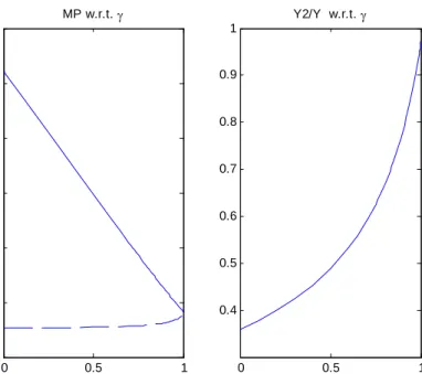
Figure 1 shows the marginal productivity of capital for the two groups of agents as a function of in the benchmark model. Using the equations repre-senting the households’optimal choice of capital evaluated at the steady state it is possible to show that as long as < 1
1; K1 K2 = m1 m2 1[1 2 ( 1 2)] 2[1 1] 1 1 >1: (12)
Thus, the steady state allocation of capital depends on the subjective discount factors, the population weights for the two groups of agents, and . Compared to the frictionless case, the allocation under credit constraints reduces the level of capital held by borrowers and implies a di¤erence in the marginal produc-tivity of capital for the two groups of producers. The higher the lower the di¤erence between borrowers’and lenders’marginal productivity and the larger the borrowers’share of total production. Since total output is maximized when the marginal productivity of the two groups is identical, collateral requirements distort total production below the e¢ cient level. However, in the absence of costly liquidation procedures the allocation of capital between the two groups of agents is close to the e¢ cient allocation and the loss in terms of aggregate output is negligible.
4
Productivity Shocks in the Benchmark Model
4.1
Impulse-Responses
Now, we consider the response of the model economy to a productivity shock. We assume that the economy is at the steady state level at time zero and then is hit by an unexpected increase in aggregate productivity of 1 percent. An aggregate shock raises production and thus the earnings of both groups of agents. See Figure 2. As the shock hits the economy, borrowers, initially limited in their capital holdings by borrowing constraints, increase their demand for productive assets. This allows the agents to more easily smooth the e¤ect of the shock. In order for the capital market to clear, lenders have to decrease their demand for capital. The user cost of holding capital increases. Movements in the relative price of capital, altering the value of the collateral asset, a¤ect the ability to borrow. Thus, borrowers’expenditure decisions are a¤ected not only by the direct impact of the shock but also by the larger availability of credit resulting from a rise in the value of their collateral. Due to the higher marginal productivity of capital experienced by the borrowers, the positive e¤ect of an increase in aggregate productivity on total production is propagated over time.
4.2
Ampli…cation and Persistence
Kiyotaki and Moore’s theoretical work shows that collateral constraints may generate large ampli…cation of productivity shocks. However, Cordoba and Ripoll (2004) document that the ampli…cation generated by the model is driven by two unorthodox assumptions: the linearity of the borrowers’ production technology in the collateral asset and the lenders’linear utility function in con-sumption. According to their results, when agents face concave preferences and technology no ampli…cation is endogenously generated by collateral constraints under standard parameter values. In what follows we investigate the role of LTV ratios for the ampli…cation of shocks through collateral constraints when borrowers and lenders face the same concave production technology and utility and the parameters are set to values commonly used in the literature. Since in
the benchmark model the …rst impact of the shock is equal to the shock itself, we look at the second-period e¤ect of the shock. We show that the magnitude of the endogenous ampli…cation delivered by collateral constraints crucially depends on the fraction of the asset used as a collateral in the credit market.
Strictly speaking, the second-period elasticity of total output with respect to technology shocks can be written as in Cordoba and Ripoll (2004):
yz= yk2 k2z=
Fk2 Fk1 Fk2
y2
y k2z: (13)
The …rst term is the productivity gap between constrained and unconstrained agents, represents the share of capital in production, while y2
y is the
produc-tion share of constrained agents, and k2z is the elasticity of borrowers’capital
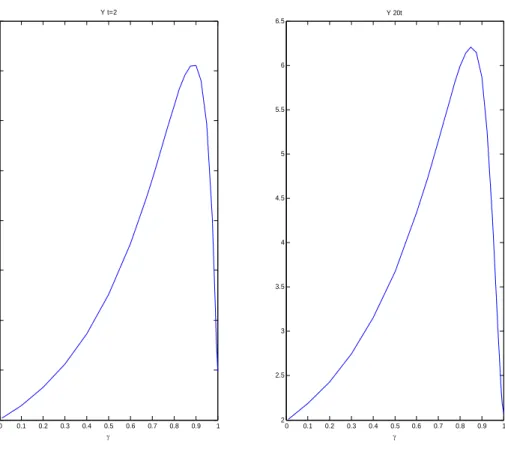
with respect to the shock –i.e. the redistribution of capital to impatient agents. As we have already shown in section 3.2, the fraction of total output produced by constrained agents increases with since more e¢ cient enforcement proce-dures induce a better allocation of capital in the economy. However, for the same reason, the productivity gap decreases with . These two opposite forces contribute to a non-linear shape of the second-period impact of the shock on total output. Figure 3 plots the second-period variation in output (left panel) and the cumulative response over a 20-quarter period (right panel) w.r.t. the fraction of the collateral value up to which agents’can borrow.
The model features negligible ampli…cation in only two parametrization: autarky and fully e¢ cient debt enforcement procedures. These parameterization of the model correspond to the case in which either the production share or the productivity gap are close to zero, respectively. In the absence of a credit market –i.e. = 0–capital is allocated in a very ine¢ cient way and borrowers’ share of total output is close to zero. So, the gains from a better allocation of resources are potentially very big. However, the redistribution of capital induced by the shock itself is limited since impatient agents cannot …nance their capital expenditure through the credit market. The ampli…cation of the shocks on total production is, indeed, negligible. Easier access to external funds generates larger redistribution of capital and enhances the endogenous ampli…cation generated
by the model. However, as increases the di¤erence in the marginal productivity of capital between lenders and borrowers shrinks. When approaches unity the allocation of capital between borrowers and lenders is such that the productivity gap is indeed negligible and the economy is very close to the e¢ cient equilibrium. Thus, as in Cordoba and Ripoll (2004) we …nd no ampli…cation in this special case.
For intermediate values of the model with collateral constraints can gener-ate ampli…cation and persistence of productivity shocks of non-negligible mag-nitude. The second-period e¤ect and the cumulative e¤ect over a 20-quarter period go hand in hand documenting no trade-o¤ between ampli…cation and persistence of productivity shocks with respect to changes in . Moreover, the e¤ect of the shock on output can be much stronger and persistent than the re-sponse generated by the representative agent model. In this latter framework, the economy is populated only by patient agents and there are no limits to credit. Over a 20-quarter period the cumulative deviation of output from the steady state can be as large as almost 2 times the variation of output induced in the representative agent version of the model.
The analysis conducted above assumes that borrowers and lenders di¤er only in terms of their subjective discount factor. Allowing also for heterogeneity also in technologies and preferences, as in Kiyotaki and Moore (1997), gener-ates larger ampli…cation of shocks for any given :In particular, Kiyotaki and Moore (1997) assume linearity for the borrowers’ production function and for the lenders’ utility function. Assuming a linear production function in capital for the borrowers (concave for the lenders) would imply a constant marginal productivity of capital for this group of agents and, thus, a larger productivity gap and more sizable potential gains from the redistribution of capital. Instead, linearity of the lenders’utility function (concavity for the borrowers) would im-ply a constant real interest rate. If lenders are willing to provide additional funds without any rise in the real interest rate, borrowers’ increase in capital expenditure and production is more sizeable. Under these two assumptions on technology and preferences, the elasticity of borrowers’capital to productivity
shocks would be higher. Thus, the ampli…cation of the shock on output would be even more sizable for any given .
5
Robustness Analysis
In the following we check for the robustness of the results to alternative model’s assumptions, parameters’values and solution method.
5.1
Reproducible Capital
Does allowing for the input of production to be elastically supplied reduce the ampli…cation e¤ect of collateral constraint?
According to Cordoba and Ripoll (2004), if capital is not …xed but rather optimally supplied, the ampli…cation role of collateral constraints is further reduced. Following Cordoba and Ripoll (2004) we now allow for reproducible capital and assume that each agent is able to produce both consumption and investment goods.5 Both types of production are identical6
yit=Zt kitc 1 y i; h it=Zt kith 1 h i ; (14)
where yit represents the technology for producing consumption goods and hit
is the production for capital goods with kjit 1 –j =c; h – being the stock of capital used as an input of production in the two sectors, respectively. Total individual production is given by
Fit=yit+qthit:
It is possible to express the amount of capital allocated to each type of produc-tion as a fracproduc-tion of the total capital owned by each agent, as follows
kitc 1= tkit 1; (15)
5In this way we avoid creating a rental market for capital, and make the model directly
comparable to those of Kiyotaki and Moore (1997).
6The assumption of decreasing returns in the production of investment goods is equivalent
to assume convex adjustment costs for investments. Capital is assumed to depreciate at a rate equal to 0.025.
where t(q) = q 1 1 t 1+q 1 1 t
: Thus, the allocation of existing capital between the two productions depends on the current relative price of capital.7 The total
production of each individual can be expressed as
Fit=kit 1Zt[ t +qt(1 t) ]: (16)
Each agent’s capital stock evolves according to
kit= (1 )kit 1+hit:
Figure 4 compares the output’s reaction to the productivity shock for dif-ferent values of . The …rst- and second-period response of output is displayed. The results show signi…cant …rst-period ampli…cation. However, the endogenous ampli…cation generated by the model declines with higher LTV ratios. Given that an economy with a high LTV ratio displays a smaller productivity gap between lenders and borrowers, less capital is redistributed to the borrowers. Thus, their demand for capital rises by a smaller margin, which dampens the increase in the relative price of capital. Since in the model with reproducible capital, variations in its relative price enter the measurement of total output, the decline in the sensitivity of the relative price of capital directly a¤ects the sensitivity of total output to productivity shocks.
In the second period both the relative-price e¤ect and the redistribution of capital between groups of producers contribute to ampli…cation. As in the model with capital in …xed supply, the second-period response displays a non-linear shape w.r.t. . However, the endogenous ampli…cation generated by the model with elastic capital supply is generally larger than in the benchmark model.
7In any given period each agent allocates the existing capital to produce either consumption
or investment goods by solving
max
kc it 1
Zt kcit 1 +qt kit 1 kcit 1
This leads to the …rst-order condition,
kcit 1 1
=qt kit 1 kitc 1 1
The relative price of capital equals the ratio of the marginal productivity of capital in the two sectors. Thus, the amount of capital allocated to each type of production equals a fraction of the total capital owned by each agent.
Thus, the result of a reduction in the second-period ampli…cation due to the introduction of elastic capital supply highlighted by Cordoba and Ripoll (2004) holds only for values of close to one.
5.2
Parameters’Value
Are our results robust to alternative calibrations? is di¤erent from the other parameters regarding its e¤ects on the ampli…cation and persistence of produc-tivity shocks?
A few papers highlighted the role of other parameters for ampli…cation. In particular, Pintus (2011), using a version of the model with capital accumulation showed that sizable ampli…cation and persistence can be generated through high, but still empirically plausible, values of relative risk aversion, ; Kocherlakota (2000) using a small open economy version of the model highlighted the need of an uncommonly high capital share in production, , to generate ampli…cation of productivity shocks; Cordoba and Ripoll (2004) concluded that in response to a one-time unexpected shock, sizable ampli…cation can be generated only by assuming implausibly high values of the relative risk aversion, , together with uncommonly high capital share in production, . Previous analysis neglected the role of ine¢ ciencies in the liquidation of the collateral asset and are, thus, based on the assumption that equals one.
Results presented above show that for values of below unity the model with collateral constraints can generate persistence and ampli…cation of non-negligible magnitude even under standard parameters’ values. In this section we investigate how other parameters a¤ect the relationship between and am-pli…cation and persistence of productivity shocks. Figure 5 documents the sen-sitivity of the results to alternative parameters’values. We consider parameters’ values in the range suggested by the empirical literature.8 In accordance with
8We choose values for the discount factor,
2, in line with previous evidence. In particular,
see Lawrance (1991) for estimates of discount factors for poor households in the range (0.95, 0.98); for an empirical distribution of discount factors Carroll and Andrew Samwick (1997) using information on the elasticity of assets with respect to uncertainty …nd that it ranges in the interval (0.91, 0.99) and Samwick (1998) using wealth holdings documents that mean discount factors of around 0.99 for about 70 percent of the population and below 0.95 for
previous authors, we …nd that for equal one larger ampli…cation is generated by higher values of ,mand . Higher values of the risk aversion means that impatient agents are more willingness to smooth the e¤ect of the shocks through borrowing and thus a more persistent e¤ect of the shock. A larger fraction of borrowers, m, means a larger fraction of total capital held by this group of agents. This implies a larger share of output is accrued to borrowers and thus, a more sensitive response of total output to shocks. Regardingm and the same result holds for alternative values of –i.e. larger ampli…cation and per-sistence is delivered by higher values ofmand for any value of . In contrast, our …ndings highlight a non-monotonic relationship between the ampli…cation generated by alternative values of and the values of and 2.
Regarding the share of capital in production, we compare the results for = 0:4, which corresponds to the standard de…nition of capital, with = 0:7, which re‡ects a broader de…nition of capital that includes both physical and intangible capital. See, for instance, Angeletos and Calvet (2006). We …nd that output ampli…cation is not a strictly increasing function of the capital share. The relation between and the sensitivity of output to productivity shocks is clearly non-linear with respect to . A higher generates larger ampli…cation and persistence of productivity shocks only under high LTV ratios. Thus, Kocherlakota (2000) and Cordoba and Ripoll (2004) results on the need of uncommonly high capital share in production, do not hold for any given value of . In fact, standard values for the capital share in production are su¢ cient to amplify the e¤ect of shocks and generate sizable endogenous persistence in economies with LTV ratios lower than 95 percent.
We are particularly interested is understanding the role of 2 for ampli-…cation. Changes in this parameter have direct e¤ects on the allocation of about 25 percent of households.
Regarding the fraction of borrowers in the economy, Campbell and Mankiw (1989) estimate around 40 percent of the population to be rule-of-thumb consumers; Jappelli and Pagano (1989) using the 1983 Survey of Consumer Finances estimates 20 percent of the population to be liquidity constrained.
We choose values for the relative risk aversion in line with previous studies and in the range of the estimated distribution by Chiappori and Paiella (2008).
capital between agents. See equation (12). Figure 6 shows that, similarly to ;
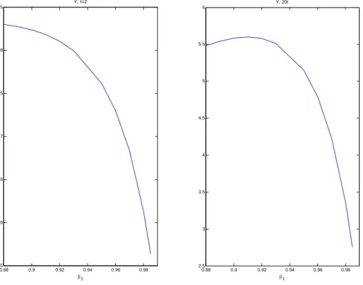
higher values of 2 reduce the productivity gap and increase the output share of borrowers. However, and 2 are very di¤erent in terms of their e¤ects on ampli…cation. As shown in …gure 7, for reasonable values of 2the e¤ect on the productivity gap always dominates and as 2 gets close to 1 the endogenous ampli…cation generated by collateral constraints is reduced.9 Nevertheless, we
…nd a non-monotonic relation between 2 and in terms of ampli…cation. In particular, higher values of 2 dampen ampli…cation and persistence for high values of while, amplifying the e¤ects of the shock for lower values of :10
Summarizing, the results presented above document that models with col-lateral constraint require uncommon assumptions about technology and utility in order to generate ampli…cation only for a particular assumptions regarding
;i.e. equal unity.
We …nd worth highlighting that results presented in this section document an independent role of in generating ampli…cation. In particular, independently of other parameters’values, the model features a non-linear relationship between the value of and the ampli…cation and persistence generated by productivity shocks. Negligible ampli…cation is always only found for values of either close to zero or close to one. Moreover, for intermediate values of the endogenous ampli…cation and persistence generated by the collateral constraint is always larger than in the representative-agent version of the same model.
5.2.1 Local Identi…cation Analysis
Is the e¤ect of changing locally almost the same as changing other parameters? In previous sections we studied the e¤ects of di¤erent parameters on the response of output to shocks. The sensitivity of output to shocks is only one of the several aspects of the model. This section report a more comprehensive analysis on the e¤ect of di¤erent parameters for the solution of the model. We investigate if the e¤ect on the structural characteristic of the model obtained
9If
2equals 1the model collapses into the representative-agent version of the model.
1 0Cordoba and Ripoll (2004), already document that higher values of
2 exhacerbate
by changing can also be obtained by changing other parameters. Due to the di¢ culty in deriving explicitly the relationship between the parameters of the model regarding the model’s dynamics, we use the local identi…cation method-ology developed by Iskrev (2010.a).11
First, we test for local identi…cation of the model’s parameters =f ; 2; ; ; m; zg
in terms of the model’s solution. A parameter i is (locally) weakly identi…ed
if either (1) the matrix ( ) that collects the reduced-form parameters of the solution of the model is insensitive to changes in ior (2) if the e¤ects on ( )of
changing i can be o¤set by changing other parameters.12 Using these criteria,
we …nd that all parameters are identi…ed in a neighborhood of the benchmark parameters’values.
The second condition is particular interesting since it allows us to under-stand if the e¤ect of changing is locally almost the same as changing other parameters. We compute the correlation between the column of the Jacobian w.r.t. and each of the other parameters – i.e. corr @@( );@@ ( )
i – for any di¤erent value of : Correlation among parameters in terms of the solution of the model is a common feature of dynamic general equilibrium models.13 As
stressed by Iskrev (2010.b) the strength of identi…cation varies across di¤erent regions in the parameter space. However, no multicollinearity is found in the model.
The pair-wise correlations in terms of the model’s solution depend on where we evaluate the partial derivatives and it is generally higher for equal to one. See Figures 8 and 9. The correlation between @@( ) and @@( )
2 is particularly
high when is close to unity. Figure 8 shows that the highest correlation between the two parameters can be found for = 0:98. This means that, for
1 1Most of the literature on identi…cation in DSGE models is concerned with the fact that
some parameters can be unidenti…able due to the lack empirical relevance. Iskrev (2010.a and 2010.b) distinguish between the statistical and the economic modelling aspects of identi-…cation. We focus on the tools provided by the author to examine how the identi…cation of parameters is in‡uenced by structural characteristics of the model.
1 2The analysis consists of evaluating the ranks of Jacobian matrices. The Jacobian matrix
@ ( )
@ must have full column rank in order for the parameters to be identi…able. See Iskrev
(2010.a) for a description of the methodology.
1 3See Iskrev (2010.a) and Iskrev (2010.b). The latter paper also provides an application to
close to unity, small changes in 2 have very similar e¤ects on the solution of
the model to changes in . However, we …nd that the correlation between the e¤ects of the parameters on the model’s solution signi…cantly varies with and for values of below unity the linkage between parameters strongly declines. A lower correlation means that it is less likely to reproduce the same e¤ect of on the solution of the mode by changing other parameters.
5.3
Solution Method
Are the results robust to less stringent assumptions regarding the collateral constraint?
As shown in section 3.2 the borrowing constraint is always binding in the deterministic steady state. It is a common procedure in the business cycle liter-ature to solve models with limits to borrowingà la Kiyotaki and Moore (1997) assuming that the constraint is also always binding in a neighborhood of the steady state.14 In contrast, we allow for the constraint to be
occassionally-binding outside the steady state by solving the model using a "barrier method" as in Kim, Kollmann and Kim (2010).15 Thus, we replace the inequality con-straint with a di¤erentiable penalty function that enters the utility function of the agents,
U(cit) =
c1it
1 P(kit; bit):
In order to be able to use perturbation methods, we choose an exponential penalty function as in Den Haan and De Wind (2009)
P(kit; bit) = 1 0
e[ 0( tEt[qt+1kit] bit)]:
The function is decreasing in the di¤erence betweenbitand the endogenous
limit, tEt[qt+1kit]. In practise, we solve an equivalent version of the model in
which higher borrowing is feasible but it is too costly to exceed the limit. The derivative of the Penalty function with respect tobit replaces the shadow price
1 4See among others, Iacoviello and Minetti (2007), Iacoviello (2005), Iacoviello and Neri
(2010), Campbell and Hercowitz (2005), Sterk (2010).
1 5See also Den Haan and Ocaktan (2009), Den Haan and De Wind (2010), Judd (1998),
of the borrowing constraint. Thus, for 1 = 2 = R1 2 uc2 > 0; the two
versions of the model have the same deterministic steady state. However, di¤er-ently from an always binding constraint, the penalty function approach doesn’t prevent impatient agents to borrow less than the debt limit in a neighborhood of the steady state. Still, the penalty term, 0, discourages the agents from
violating the constraint, such that large values of 0 ensure that the
indebted-ness does not exceed the limit. In the benchmark solution, 0equals 100. The
agents’optimal choices of borrowing and capital, together with the equilibrium conditions, represent a non-linear dynamic stochastic system of equations. To capture the non-linearity induced by the asymmetric penalty function, we solve for the recursive law of motion relying on a second order approximation.16
Figure 10 display the response of total output after a productivity shock implied by the two solution methods. The di¤erence between the two impulse-responses is not sizable. As a result, the …rst period impact and the 20-quarter cumulative e¤ects are very similar. See Figure 11. Thus, for intermediate values of the model with collateral constraint generate sizable ampli…cation and persistence even under less strict assumptions regarding the binding nature of the constraint.
6
Conclusions
This paper improves upon previous literature by documenting the contribution of ine¢ ciency in the debt enforcement procedure to the ampli…cation of business cycle ‡uctuations which other authors have not considered. We argue that the magnitude of ampli…cation crucially depends on the fraction of the asset used as a collateral in the credit market.
In accordance with previous papers that call into question the relevance of collateralized debt as a transmission mechanism, we …nd that when ine¢
-1 6Den Haan and De Wind (2009) solve the model by Deaton (1991) with a penalty
func-tion approach and show that, di¤erently from higher order perturbafunc-tion solufunc-tions, the policy function of the second-order approximate solution is close to the accurate solution and that despite being a bit more convex it preserves its shape. Further issues related to the use of approximate solutions for generating simulated data are not of a concern for the purpose of this paper.
ciency in the debt enforcement process are not taken into account –i.e. =1 – collateral constraints predict negligible ampli…cation of productivity shocks to output. Nevertheless, when realistic Loan-to-Value ratios are assumed, the role of collateral constraints in terms of the ampli…cation of productivity shocks is signi…cantly enhanced, even under standard assumptions on the utility function and production process. Thus, results presented by previous literature are not robust to di¤erent assumptions on the degree of ine¢ ciency in the credit market.
7
References
Angeletos, G.M., and L.M. Calvet, 2006. Idiosyncratic Production Risk, Growth and the Business Cycle,Journal of Monetary Economics, vol. 53.
Calstrom and Fuerst, 1997. Agency Costs, Net Worth, and Business Fluc-tuations: A Computable General Equilibrium Analysis. American Economic Review, vol. 87.
Calza, A., Monacelli, T., and L. Stracca, 2010. Housing Finance and Mone-tary Policy, forthcomingJournal of the European Economic Association.
Campbell, J. R. and Z. Hercowitz, 2004. The Role of Collateralized House-hold Debt in Macroeconomic Stabilization, NBER w.p 11330.
Campbell, J. Y. and N. G. Mankiw, 1989. Consumption, Income, and In-terest Rates: Reinterpreting the Time Series Evidence, in Oliver J. Blanchard and Stanley Fischer, eds., NBER macroeconomics annual. Vol. 4. Cambridge, MA: MIT Press, pp. 185–216.
Carlstrom, C.T, Fuerst,T., 2007. Asset Prices, Nominal Rigidities, and Mon-etary Policy,Review of Economic Dynamics, vol. 10.
Carroll, C. D. and A. A. Samwick, 1997. The Nature of Precautionary Wealth, Journal of Monetary Economics, vol. 40.
Chiappori, P.A. and Paiella, M., 2008. Relative Risk aversion is Constant: Evidence from Panel Data. Discussion paper 5-2008, University of Naples, Parthenope.
Cordoba, J.C. and M. Ripoll, 2004. Credit Cycle Redux,International
Eco-nomic Review, vol. 45.
Deaton, A., 1991. Saving and Liquidity Constraints,Econometrica, vol. 59. Den Haan, W.J., Ocaktan, T.,S., 2009. Solving Dynamic Models with Heterogeneous Agents and Aggregate Uncertainty with Dynare or Dynare++, mimeo.
Den Haan, W.J., and J. De Wind, 2010. Nonlinear and Stable Perturbation-based Approximations, mimeo.
Djankov,S., Hart O., McLiesh C. and A. Shleifer, (2008), Debt Enforcement Around the World,Journal of Political Economy, vol. 116.
Greenwood, J., G. W. Hu¤man, and Z. Hercowitz, 1988. Investment, Ca-pacity Utilization, and the Real Business Cycle, American Economic Review, vol. 78.
Hendricks, L., 2007. How Important Is Discount Rate Heterogeneity for Wealth Inequality?,Journal of Economic Dynamics and Control, vol. 31.
Judd, K.L., 1998. Numerical Methods in Economics. The ,MITT Press, Cambridge, Massachusetts.
Iacoviello, M., 2005. House Prices, Borrowing Constraints and Monetary Policy in the Business Cycle,American Economic Review, vol. 95.
Iacoviello, M. and R. Minetti, 2006. International Business Cycles with Domestic and Foreign Lenders,Journal of Monetary Economics, vol. 53.
Iacoviello, M. and S. Neri, 2010. Housing Market Spillovers: Evidence from an Estimated DSGE Model,AEJ Macro, vol. 2.
Iskrev, N., 2010.a. Local Identi…cation in DSGE Models. Journal of
Mone-tary Economics, vol. 57.
Iskrev, N., 2010.b. Evaluating the Strength of Identi…cation in DSGE Mod-els. An A Priori Approach, Bank of Portugal w.p. 32-2010.
Jappelli, T., and M. Pagano, 1989. Consumption and Capital Market Im-perfections: An International Comparison. American Economic Review, vol. 79.
Lawrance, E. C., 1991. Poverty and the Rate of Time Preference: Evidence from Panel Data,Journal of Political Economy, vol. 99.
Kim, S., Kollmann, R., and J. Kim, 2009. Solving the Incomplete Matkets Model with Aggregate Uncertainty using Perturbation Methods,Journal of
Eco-nomic Dynamics and Control,vol. 34, 50-58.
Kiyotaki, N., 1998. Credit and Business Cycles, The Japanese Economic Review, vol. 49.
Kiyotaki, N. and J. Moore, 1997. Credit Cycles, Journal of Political Econ-omy, vol. 105.
Kocherlakota, N.R., 2000. Creating Business Cycles Through Credit Con-straints, Federal Reserve Bank of Minneapolis Quarterly Review, vol 24.
Mendoza, E., 2006. Lessons from the Debt De‡ation Theory of Sudden Stops,American Economic Review Papers & Proceedings, vol. 96.
Mendoza, E., and K. A. Smith, 2006. Quantitative Implications of a Debt-De‡ation Theory of Sudden Stops and Asset Prices, Journal of International
Economics, vol. 70.
Osborne, J., 2005. Housing in the Euro Area. Twelve Markets, One Money, International Finance Discussion Papers 740, Central Bank of Ireland.
Pintus, P.A., 2011. Collateral Constraints and the Ampli…cation-Persistence Trade-O¤. Economics Letters, vol. 110.
Preston, B., and M. Roca, 2006. Incomplete Markets, Heterogeneity and Macroeconomic Dynamics, mimeo.
Samwick, A., 1998. Discount Rate Heterogeneity and Social Security Re-form,Journal of Development Economics, vol. 57.
Smets, F. and R. Wouters, 2003. An Estimated Dynamic Stochastic Gen-eral Equilibrium Model of the Euro Area, Journal of the European Economic Association, vol.1.
Sterk, V., 2010. Credit frictions and the comovement between durable and non-durable consumption. Journal of Monetary Economics, vol. 57.
Uribe, M., 2006. On Overborrowing, American Economic Review Papers and Proceedings, vol. 96.
Warner, J. T., and S. Pleeter, 2001. The Personal Discount Rate: Evidence from Military Downsizing Programs,American Economic Review, vol. 91.
Figure 1 Benchmark Model. Steady state productivity gap between the two groups of agents (solid line
borrowers, dashed line lenders) and borrowers’ share of total production as a function of γ.
Figure 2. Benchmark Model. Responses of the model economy to a one-period 1% increase in aggregate
productivity; γ=0.85. The vertical axes measure deviations from the steady state, while on the
horizontal axes are years.
0 0.5 1 0 0.5 1 1.5 2 2.5 3 MP w.r.t. 0 0.5 1 0.4 0.5 0.6 0.7 0.8 0.9 1 Y2/Y w.r.t. 5 10 15 20 0 0.01 0.02 0.03 0.04 0.05 b2 5 10 15 20 0 0.01 0.02 0.03 0.04 k2 5 10 15 20 -0.01 -0.005 0 0.005 0.01 q 5 10 15 20 0 0.002 0.004 0.006 0.008 0.01 0.012 y 5 10 15 20 -5 -4 -3 -2 -1 0 1x 10 -3 R 5 10 15 20 -4 -2 0 2 4x 10 -3 c1 5 10 15 20 0 0.005 0.01 0.015 0.02 0.025 0.03 c2 5 10 15 20 -0.01 -0.005 0 0.005 0.01 y1 5 10 15 20 0 0.005 0.01 0.015 0.02 0.025 y2
Figure 3. Benchmark Model. Sensitivity of Output to a productivity shock for any given γ; second-period (left panel) and cumulative response over a 20 quarters period (right panel). Dotted-line representative agent model.
Figure 4. Reproducible Capital Model. Sensitivity of Output to a productivity shock for any given γ;
first-period (left panel), second-first-period response (right panel). Dotted-line representative agent model; dashed-line benchmark model.
0 0.1 0.2 0.3 0.4 0.5 0.6 0.7 0.8 0.9 1 0.45 0.5 0.55 0.6 0.65 0.7 0.75 0.8 0.85 0.9 Y, t=2 0 0.1 0.2 0.3 0.4 0.5 0.6 0.7 0.8 0.9 1 1.5 2 2.5 3 3.5 4 4.5 5 5.5 6 Y, 20t 0 0.1 0.2 0.3 0.4 0.5 0.6 0.7 0.8 0.9 1 1 1.05 1.1 1.15 1.2 1.25 1.3 1.35 1.4 Ft=1 0 0.1 0.2 0.3 0.4 0.5 0.6 0.7 0.8 0.9 1 0.45 0.5 0.55 0.6 0.65 0.7 0.75 0.8 0.85 0.9 Ft=2 reproducible capital benchmark model
Figure 5. Benchmark Model. Sensitivity of Output to a productivity shock for any given γ; second-period (left panel) and cumulative response over a 20 quarters period (right panel) for alternative parameters’ value.
0 0.5 1 0.5 0.55 0.6 0.65 0.7 0.75 0.8 0.85 0.9 2 t=2 0 0.5 1 0.5 0.55 0.6 0.65 0.7 0.75 0.8 0.85 0.9 0.95 1 0 0.5 1 0.5 0.55 0.6 0.65 0.7 0.75 0.8 0.85 0.9 m 0 0.5 1 0.5 0.6 0.7 0.8 0.9 1 1.1 0 0.5 1 2 2.5 3 3.5 4 4.5 5 5.5 6 20t 2 0 0.5 1 2 3 4 5 6 7 8 9 0 0.5 1 2 2.5 3 3.5 4 4.5 5 5.5 6 m 0 0.5 1 2 3 4 5 6 7 8 9 10 11 12 13 2 =0.91 2 =0.95 2 =0.97 =0.4 =0.7 n=0.5 n=0.4 n=0.25 =2.2 =1 =5
Figure 6 Benchmark Model. Steady state productivity gap between the two groups of agents (solid
line borrowers, dashed line lenders) and borrowers’ share of total production as a function of β2.
Figure 7. Benchmark Model. Sensitivity of Output to a productivity shock for any given β2;
second-period (left panel) and cumulative response over a 20 quarters second-period (right panel).
0.88 0.9 0.92 0.94 0.96 0.98 0.2 0.3 0.4 0.5 0.6 0.7 0.8 0.9 2 MP w.r.t. 2 0.88 0.9 0.92 0.94 0.96 0.98 0.65 0.7 0.75 0.8 0.85 0.9 0.95 1 y2/y w.r.t. 2 2 0.88 0.9 0.92 0.94 0.96 0.98 0.55 0.6 0.65 0.7 0.75 0.8 0.85 Y, t=2 2 0.88 0.9 0.92 0.94 0.96 0.98 2.5 3 3.5 4 4.5 5 5.5 6 Y, 20t 2
Figure 8. Correlation between the column of the Jacobian w.r.t. γ and β2 for any given γ.
Figure 9. Correlation between the column of the Jacobian w.r.t. γ and each of the other
parameters for any given γ.
0 0.1 0.2 0.3 0.4 0.5 0.6 0.7 0.8 0.9 1 0.1 0.2 0.3 0.4 0.5 0.6 0.7 0.8 0.9 1 2 , (0,1) 0.92 0.93 0.94 0.95 0.96 0.97 0.98 0.99 1 0.93 0.94 0.95 0.96 0.97 0.98 0.99 1 2 , (0.92,1) Correlations Jacobian 0 0.1 0.2 0.3 0.4 0.5 0.6 0.7 0.8 0.9 1 0.2 0.3 0.4 0.5 0.6 0.7 0.8 0 0.1 0.2 0.3 0.4 0.5 0.6 0.7 0.8 0.9 1 0 0.1 0.2 0.3 0.4 0.5 0.6 0.7 0.8 0.9 m 0 0.1 0.2 0.3 0.4 0.5 0.6 0.7 0.8 0.9 1 0.4 0.45 0.5 0.55 0.6 0.65 0.7 0.75 0 0.1 0.2 0.3 0.4 0.5 0.6 0.7 0.8 0.9 1 0.35 0.4 0.45 0.5 0.55 z Correlations Jacobian
Figure 10. Benchmark Model. Responses of total output to a one-period 1% increase in aggregate
productivity; γ=0.85. The vertical axes measure deviations from the steady state, while on the
horizontal axes are years. Penalty function vs always binding constraint.
Figure 11.Benchmark Model. Sensitivity of Output to a productivity shock for any given γ;
second-period (left panel) and cumulative response over a 20 quarters second-period (right panel). Penalty Function. 2 4 6 8 10 12 14 16 18 20 0 0.002 0.004 0.006 0.008 0.01 0.012 y penalty binding 0 0.1 0.2 0.3 0.4 0.5 0.6 0.7 0.8 0.9 1 0.5 0.55 0.6 0.65 0.7 0.75 0.8 0.85 0.9 Y t=2 0 0.1 0.2 0.3 0.4 0.5 0.6 0.7 0.8 0.9 1 2 2.5 3 3.5 4 4.5 5 5.5 6 6.5 Y 20t
WORKING PAPERS
2010
1/10 MEASURING COMOVEMENT IN THE TIME-FREQUENCY SPACE — António Rua
2/10 EXPORTS, IMPORTS AND WAGES: EVIDENCE FROM MATCHED FIRM-WORKER-PRODUCT PANELS — Pedro S. Martins, Luca David Opromolla
3/10 NONSTATIONARY EXTREMES AND THE US BUSINESS CYCLE — Miguel de Carvalho, K. Feridun Turkman, António Rua
4/10 EXPECTATIONS-DRIVEN CYCLES IN THE HOUSING MARKET — Luisa Lambertini, Caterina Mendicino, Maria Teresa Punzi
5/10 COUNTERFACTUAL ANALYSIS OF BANK MERGERS
— Pedro P. Barros, Diana Bonfi m, Moshe Kim, Nuno C. Martins
6/10 THE EAGLE. A MODEL FOR POLICY ANALYSIS OF MACROECONOMIC INTERDEPENDENCE IN THE EURO AREA — S. Gomes, P. Jacquinot, M. Pisani
7/10 A WAVELET APPROACH FOR FACTOR-AUGMENTED FORECASTING — António Rua
8/10 EXTREMAL DEPENDENCE IN INTERNATIONAL OUTPUT GROWTH: TALES FROM THE TAILS — Miguel de Carvalho, António Rua
9/10 TRACKING THE US BUSINESS CYCLE WITH A SINGULAR SPECTRUM ANALYSIS — Miguel de Carvalho, Paulo C. Rodrigues, António Rua
10/10 A MULTIPLE CRITERIA FRAMEWORK TO EVALUATE BANK BRANCH POTENTIAL ATTRACTIVENESS — Fernando A. F. Ferreira, Ronald W. Spahr, Sérgio P. Santos, Paulo M. M. Rodrigues
11/10 THE EFFECTS OF ADDITIVE OUTLIERS AND MEASUREMENT ERRORS WHEN TESTING FOR STRUCTURAL BREAKS IN VARIANCE
— Paulo M. M. Rodrigues, Antonio Rubia
12/10 CALENDAR EFFECTS IN DAILY ATM WITHDRAWALS — Paulo Soares Esteves, Paulo M. M. Rodrigues
13/10 MARGINAL DISTRIBUTIONS OF RANDOM VECTORS GENERATED BY AFFINE TRANSFORMATIONS OF
INDEPENDENT TWO-PIECE NORMAL VARIABLES — Maximiano Pinheiro
14/10 MONETARY POLICY EFFECTS: EVIDENCE FROM THE PORTUGUESE FLOW OF FUNDS — Isabel Marques Gameiro, João Sousa
15/10 SHORT AND LONG INTEREST RATE TARGETS — Bernardino Adão, Isabel Correia, Pedro Teles
16/10 FISCAL STIMULUS IN A SMALL EURO AREA ECONOMY
— Vanda Almeida, Gabriela Castro, Ricardo Mourinho Félix, José Francisco Maria
17/10 FISCAL INSTITUTIONS AND PUBLIC SPENDING VOLATILITY IN EUROPE — Bruno Albuquerque
18/10 GLOBAL POLICY AT THE ZERO LOWER BOUND IN A LARGE-SCALE DSGE MODEL — S. Gomes, P. Jacquinot, R. Mestre, J. Sousa
19/10 LABOR IMMOBILITY AND THE TRANSMISSION MECHANISM OF MONETARY POLICY IN A MONETARY UNION — Bernardino Adão, Isabel Correia
20/10 TAXATION AND GLOBALIZATION — Isabel Correia
21/10 TIME-VARYING FISCAL POLICY IN THE U.S. — Manuel Coutinho Pereira, Artur Silva Lopes
22/10 DETERMINANTS OF SOVEREIGN BOND YIELD SPREADS IN THE EURO AREA IN THE CONTEXT OF THE ECONOMIC AND FINANCIAL CRISIS
— Luciana Barbosa, Sónia Costa
23/10 FISCAL STIMULUS AND EXIT STRATEGIES IN A SMALL EURO AREA ECONOMY — Vanda Almeida, Gabriela Castro, Ricardo Mourinho Félix, José Francisco Maria
24/10 FORECASTING INFLATION (AND THE BUSINESS CYCLE?) WITH MONETARY AGGREGATES — João Valle e Azevedo, Ana Pereira
25/10 THE SOURCES OF WAGE VARIATION: AN ANALYSIS USING MATCHED EMPLOYER-EMPLOYEE DATA — Sónia Torres,Pedro Portugal, John T.Addison, Paulo Guimarães
26/10 THE RESERVATION WAGE UNEMPLOYMENT DURATION NEXUS — John T. Addison, José A. F. Machado, Pedro Portugal
27/10 BORROWING PATTERNS, BANKRUPTCY AND VOLUNTARY LIQUIDATION — José Mata, António Antunes, Pedro Portugal
28/10 THE INSTABILITY OF JOINT VENTURES: LEARNING FROM OTHERS OR LEARNING TO WORK WITH OTHERS — José Mata, Pedro Portugal
29/10 THE HIDDEN SIDE OF TEMPORARY EMPLOYMENT: FIXED-TERM CONTRACTS AS A SCREENING DEVICE — Pedro Portugal, José Varejão
30/10 TESTING FOR PERSISTENCE CHANGE IN FRACTIONALLY INTEGRATED MODELS: AN APPLICATION TO WORLD INFLATION RATES
— Luis F. Martins, Paulo M. M. Rodrigues
31/10 EMPLOYMENT AND WAGES OF IMMIGRANTS IN PORTUGAL — Sónia Cabral, Cláudia Duarte
32/10 EVALUATING THE STRENGTH OF IDENTIFICATION IN DSGE MODELS. AN A PRIORI APPROACH — Nikolay Iskrev
33/10 JOBLESSNESS
— José A. F. Machado, Pedro Portugal, Pedro S. Raposo
2011
1/11 WHAT HAPPENS AFTER DEFAULT? STYLIZED FACTS ON ACCESS TO CREDIT — Diana Bonfi m, Daniel A. Dias, Christine Richmond
2/11 IS THE WORLD SPINNING FASTER? ASSESSING THE DYNAMICS OF EXPORT SPECIALIZATION — João Amador
3/11 UNCONVENTIONAL FISCAL POLICY AT THE ZERO BOUND — Isabel Correia, Emmanuel Farhi, Juan Pablo Nicolini, Pedro Teles
4/11 MANAGERS’ MOBILITY, TRADE STATUS, AND WAGES — Giordano Mion, Luca David Opromolla
5/11 FISCAL CONSOLIDATION IN A SMALL EURO AREA ECONOMY
— Vanda Almeida, Gabriela Castro, Ricardo Mourinho Félix, José Francisco Maria
6/11 CHOOSING BETWEEN TIME AND STATE DEPENDENCE: MICRO EVIDENCE ON FIRMS’ PRICE-REVIEWING STRATEGIES
— Daniel A. Dias, Carlos Robalo Marques, Fernando Martins
7/11 WHY ARE SOME PRICES STICKIER THAN OTHERS? FIRM-DATA EVIDENCE ON PRICE ADJUSTMENT LAGS — Daniel A. Dias, Carlos Robalo Marques, Fernando Martins, J. M. C. Santos Silva
8/11 LEANING AGAINST BOOM-BUST CYCLES IN CREDIT AND HOUSING PRICES — Luisa Lambertini, Caterina Mendicino, Maria Teresa Punzi
9/11 PRICE AND WAGE SETTING IN PORTUGAL LEARNING BY ASKING — Fernando Martins
10/11 ENERGY CONTENT IN MANUFACTURING EXPORTS: A CROSS-COUNTRY ANALYSIS — João Amador
11/11 ASSESSING MONETARY POLICY IN THE EURO AREA: A FACTOR-AUGMENTED VAR APPROACH — Rita Soares
12/11 DETERMINANTS OF THE EONIA SPREAD AND THE FINANCIAL CRISIS — Carla Soares, Paulo M. M. Rodrigues
13/11 STRUCTURAL REFORMS AND MACROECONOMIC PERFORMANCE IN THE EURO AREA COUNTRIES: A MODEL-BASED ASSESSMENT
— S. Gomes, P. Jacquinot, M. Mohr, M. Pisani
14/11 RATIONAL VS. PROFESSIONAL FORECASTS — João Valle e Azevedo, João Tovar Jalles
15/11 ON THE AMPLIFICATION ROLE OF COLLATERAL CONSTRAINTS — Caterina Mendicino