Envy, Guilt, and the Phillips Curve
Steffen Ahrens
Dennis Snower
CESIFO WORKING PAPER NO. 3717
C
ATEGORY
4:
L
ABOUR
M
ARKETS
J
ANUARY
2012
An electronic version of the paper may be downloaded
• from the SSRN website: www.SSRN.com
• from the RePEc website: www.RePEc.org
CESifo
Working Paper No. 3717
Envy, Guilt, and the Phillips Curve
Abstract
We incorporate inequity aversion into an otherwise standard New Keynesian dynamic
equilibrium model with Calvo wage contracts and positive inflation. Workers with relatively
low incomes experience envy, whereas those with relatively high incomes experience guilt.
The former seek to raise their income, and latter seek to reduce it. The greater the inflation
rate, the greater the degree of wage dispersion under Calvo wage contracts, and thus the
greater the degree of envy and guilt experienced by the workers. Since the envy effect is
stronger than the guilt effect, according to the available empirical evidence, a rise in the
inflation rate leads workers to supply more labor over the contract period, generating a
significant positive long-run relation between inflation and output (and employment), for low
inflation rates. This Phillips curve relation, together with an inefficient zero-inflation steady
state, provides a rationale for a positive long-run inflation rate. Given standard calibrations,
optimal monetary policy is associated with a long-run inflation rate around 2 percent.
JEL-Code: E500.
Keywords: inflation, long-run Phillips curve, fairness, inequity aversion.
Steffen Ahrens
IFW Kiel
Kiel / Germany
steffen.ahrens@ifw-kiel.de
Dennis Snower
IFW Kiel
Kiel / Germany
president@ifw-kiel.de
1
Introduction
Despite a well-known, growing body of empirical literature calling the classical dichotomy into question, it is still the conventional wisdom in contemporary macroeconomic theory that monetary policy is roughly neutral with respect to aggregate employment and output in the long run. Even though the standard New Keynesian model implies a non-neutrality due to time discounting and ine¢ ciencies due to relative price instability, these long-run e¤ects of monetary policy are quantitatively small for reasonable values of the interest rate and low in‡ation rates (Ascari (1998) and Graham and Snower (2004)).1 This paper,
by contrast, o¤ers a new rationale for long-run real e¤ects of monetary policy, resting on envy and guilt. We …nd that for reasonably calibrated values of the relevant parameters, these long-run e¤ects are substantial. This result has important implications for the conduct of mo- netary policy. Our calibration results suggest an optimal in‡ation rate in the neighborhood of 2 percent.
In particular, we incorporate fairness considerations to an otherwise stan-dard dynamic stochastic general equilibrium (DSGE) model of New Keynesian type with Calvo nominal wage contracts and positive trend in‡ation. In this context, we show that the classical dichotomy (whereby nominal variables have no long-e¤ect e¤ect on real variables) breaks down in an empirically signi…cant and theoretically novel way. Our rationale for the long-run non-neutrality of monetary policy does not rest on money illusion, departures from rational ex-pectations, or permanent nominal rigidities. Instead, we assume that people are inequity-averse with respect to real incomes, following the seminal work from Fehr and Schmidt (1999) and Bolton and Ockenfels (2000). Accordingly, people with relatively low income experience envy, whereas those with relatively high income experience guilt. Both experiences generate disutility and, in according with the evidence, the in‡uence of envy is stronger than that of guilt.
In the presence of Calvo nominal wage contracts, higher in‡ation implies greater wage dispersion and thus greater dispersion of incomes, generating more envy and guilt. Since people seek to mitigate envy and guilt, they adjust their employment accordingly. Those who experience envy seek to raise their income and do so by increasing their employment, where those who experience guilt reduce their employment. Since the envy e¤ect is stronger than the guilt e¤ect, higher in‡ation is associated with greater employment and output, thereby ge-nerating a long-run Phillips curve tradeo¤.
In this context, we examine the welfare implications of our approach. We …nd that the optimal long-run in‡ation rate (maximizing steady-state, economy-wide household utility) is positive, in the neighborhood of 2 percent for the standard calibrations. This result is in stark contrast to earlier studies of DSGE mod-els with trend in‡ation (e.g., King and Wolman (1996), Kahn et al. (2003), Yun (2005), and Schmitt-Grohé and Uribe (2007, 2010)), which …nd optimal monetary policy to either be given by price stability or even by following a
de-1This holds true for the standard assumption of exponential discounting. Graham and
Snower (2008) show that hyperbolic discounting leads to a long-run trade-o¤ of reasonable magnitude.
‡ationary path. Our results are more in line with the aims of practical monetary policy, as practiced by central bankers.
The the paper is organized as follows. Section 2 reviews the relevant litera-ture. Then section 3 describes our microfounded macro and calibrates it. Sec-tion 4 presents the numerical implicatons of the model for the long-run Phillips curve, discusses the underlying intuition, and investigates the sensitivity of the results with respect to key parameters. Section 5 examines optimal monetary policy in the presence of envy and guilt. Finally, section 6 concludes.
2
Relation to the Literature
Although evidence regarding verticality of the long-run Phillips curve had been mixed over the past century, recent years have witnessed a rapidly growing literature calling the classical dichotomy into question.2 As Gregory Mankiw
puts it "... if one does not approach the data with a prior view favoring long-run neutrality, one would not leave the data with that posterior. The data’s best guess is that monetary shocks leave permanent scars on the economy" (Mankiw (2001), p. 48). This paper provides a new rationale for such empirical …ndings. The paper also contributes to a growing theoretical literature explaining how a non-vertical long-run Phillips curve can arise (surveyed, for example, by Orphanides and Solow (1990)). In the context of state-dependent menu costs, see Benabou and Konieczny (1994), Konieczny (1990), Kuran (1986), and Naish (1986). There is also a literature that explains a long-run relation between in‡ation and employment in terms of fairness, either due to a permanent downward nominal wage rigidity (money illusion) or to departures from rational expectations (Akerlof et al. (1996), Akerlof and Dickens (2007)) and (Akerlof et al. (2000)). Our analysis, by contrast, rests on neither nominal rigidities nor non-rational expectations.3
2For the United States, see for example Beyer and Farmer (2007), Berentsen et al. (2011),
Favara and Giordani (2009), Karanassou et al. (2008), Karanassou and Sala (2010)) and Russell and Banerjee (2008) for the United States. For a wider set of industrialized countries, examples include Ball (1997, 1999), Ericson et al. (2001), Dolado et al. (2000), Fair (2000), Fisher and Seater (1993), Gottschalk and Fritsche (2005), King and Watson (1994), Koutsas (1998), Koutsas and Serletis (2003), Koutsas and Veloce (1996), Schreiber and Wolters (2007). Empirical studies that study the Phillips curve in terms of the underlying structural macro models include Ahmed and Rogers (1998), Bullard and Keating (1995), Coenen et al. (2004) and Karanassou et al. (2003, 2005). Concerning developing and emerging countries, see Bae and Ratti (2000) for Argentina and Brazil, by Wallace and Shelley (2004, 2007) for Nicaragua and Mexico, by Puah et al. (2008) for Singapore, and by Chen (2007) for Taiwan.
3See also King and Wolman (1996), Ascari (1998), and Graham and Snower (2004), who
study the e¤ects of trend in‡ation in New Keynesian models with nominal frictions and …nd a long-run relation between the growth rate of money and steady state real aggregates. Amano et al. (2007) discuss the in‡uence of trend in‡ation on business cycle characteristics such as stochastic means, volatilities, and correlations of macroeconomic aggregates. Based on a second order Taylor approximation around the deterministic steady state they …nd trend in‡ation to decrease the mean of output while the variance and the persistence of output and in‡ation increase. Finally, Graham and Snower (2008) derive a non-vertical Phillips curve from hyperbolic discounting by households.
The notion of fairness that we incorporate in a New Keynesian model is based on inequity aversion. This phenomenon, covering both envy and guilt, is supported by a massive empirical literature.4 A large body of empirical studies
in the behavioral economics literature argues that relative income substantially matters for one’s subjective well-being.5 We model inequity aversion along the
lines of Fehr and Schmidt (1999) and Bolton and Ockenfels (2000). In our analysis, workers compare their real incomes with the average real income of all the workers, feeling envy when their incomes are relatively low and guilt when they are relatively high.6 Envy is stronger that guilt, a …nding supported by
much empirical evidence.7
The novel contribution of this paper is to examine the in‡uence of such inequity aversion on the Phillips curve. As noted, we …nd that this in‡uence implies a signi…cant, positive long-run relation between in‡ation and macroeco-nomic activity for reasonably low in‡ation rates (say, below 4 percent) and in this context the optimal long-run in‡ation rate is positive and near 2 percent. This policy implication is noteworthy, since much of the previous literature on optimal monetary policy suggests that prices should decline or remain stable in the long run. According to the Friedman rule, the optimal rate of de‡ation is equal to the real interest rate. Models that include cash-in-advance constraints, shopping time technologies, and frictions related to the transactional money de-mand8 imply that the optimal in‡ation rate exceeds the Friedman rule, but is
still negative. Other models focusing on the costs of price dispersion9 suggest
that the optimal in‡ation rate is zero. Such policy implications are completely at odds with the practice of monetary policy, where positive in‡ation targets commonly play a central role. In developed countries typically target low in‡a-tion rates in an interval from 2 to 3 percent, while developing countries often apply target values which are slightly higher.10 There are few theoretical
ratio-nales for such practices.11 Against this backdrop, we provide a new justi…cation
for positive in‡ation targeting.
4See, for example, Güth et al. (1982), Forsythe et al. (1994), Roth et al. (1991), Henrich et
al. (2001), Karni et al. (2008), and Cappelen et al. (2010, 2011). For surveys of the medical, psychological and neuroeconomic background for this behavior, see Camerer et al. (2005), Loewenstein et al. (2008). See also the neuroeconomic evidence of Sanfrey et al. (2003).
5For example, Argyle (1972, 1989), Easterlin (1974, 1995), Kapteyn and Van Herwaarden
(1980), van de Stadt et al. (1985), Scitovsky (1992), Clark and Oswald (1996), Solnick and Hemenway (1998), Blanch‡ower and Oswald (2004), and Layard et al. (2009)). For a thorough survey on the theoretical and empirical literature of the impact of level and relative income on happiness refer to Clark et al. (2008).
6This idea draws on theory developed by the psychologists Homans (1961), Adams (1965)
and Walster et al. (1978).
7See, for example, Jaques (1956, 1961), Messik and Sentis (1979), and Loewenstein et al.
(1989)
8For example, King and Wolman (1996), Kahn et al. (2003), and Schmitt-Grohé and Uribe
(2007, 2010), Aruoba and Schorfheide (2011) .
9For example, Galí (2003) and Woodford (2003).
1 0See, for example, Roger and Stone (2005) and Carare and Stone (2006).
1 1An exception is Graham and Snower (2011), showing that optimal in‡ation is positive in
the presence of hyperbolic discounting by households. See also Fagan and Messina (2009) and Coibion et al. (2010).
3
The Model Economy
As noted, we incorporate inequity aversion into a standard dynamic stochastic general equilibrium model with nominal rigidities and positive trend in‡ation. Firms are perfectly competitive, while households are monopolistic competitors. Workers are in…nitely lived and located on the unit interval. Wages are …xed according to the Calvo (1983) nominal contract scheme.12 The government
prints money, issues riskless bonds, and rebates seignorage gains in equal shares to workers as a lump sum. It conducts monetary policy by controlling the growth rate of nominal money supplyMt+1=Mt;which determines long-run in‡ation13
t+1.
3.1
Firms
We assume a large number of identical …rms. Firms produces a homogenous good according to a Dixit and Stiglitz (1977) CES production function with di¤erentiated labornj as single input.
yt= Z 1 0 n 1 j;t dj 1 (1)
The parameter denotes the elasticity of substitution between the di¤erent labor types andytis output. Cost minimization subject to the …rms production
function (1) yields the …rms’demand function for the individual labor type
nj;t+i=
wj;t
(1 + )i
!
yt+i; (2)
wherewj;t is the period-treal value of householdj0s nominal contract wage set
in t. Due to perfect competition in the product market, …rms take wages and prices as given and produce output at which the price equals marginal cost. Thus the …rms’ markup is zero and the aggregate real wage is constant and equal to unity.
3.2
Workers
Workers are monopolistic competitors, maximizing the utility subject to the labor demand curves (2) that they face. Wages are …xed according to the
1 2In a subsequent paper, we also apply the Taylor (1979) staggered contracts scheme and
show that the results are quantitatively and qualitatively very similar across both approaches.
1 3See Nelson (2007, 2008). We choose money growth over an interest rate rule because, as
Reynard (2007) shows, the short term interest rate empirically fails to deliver accurate infor-mation on subsequent in‡ation, while monetary aggregates have a much greater explanatory power for the developments of subsequent in‡ation and output. This view is strongly sup-ported by Favara and Giordani (2009). Karanassou and Sala (2010) argue that money growth captures well the e¤ects of changes in the short term interest rate on in‡ation, but also covers additional stances of monetary policy such as banking regulations or possible transmission e¤ects of …scal measures on the yield curve.
Calvo (1983) nominal contract scheme: in every period, a worker has probability
(1 )to be allowed to reset her contract wage. The worker’s utility depends positively on consumption cj;t and negatively on labor nj;t. In addition, the
worker dislikes to have more or less real income than the average. The worker
j’s utility function14 is U(cj; nj;Ij) =cj;t n1+j;t 1 + j;t I2 j;t 2 ; (3)
withIj;t being the relative real income position of workers j, which is de…ned
as Ij;t+i = wj;t (1 + )inj;t+i Z 1 0 wk;t+ink;t+idk: (4)
where wk;t+i is the real value of the current wage of all other workers k. In
the spirit of Bolton and Ockenfels (2000), workerj compares her real income to the average real income of all other workersj6=k. The parameter j;t is an indicator function:
j;t=
" for Ij;t<0
for Ij;t>0
(5) where"represents envy and represents guilt, under the standard restrictions
0< <1 and" >0. Furthermore,"= where >1;a phenomenon known as egocentric bias.15
Workerj’s period-ibudget constraint is
cj;t+i+mj;t+1+i+bj;t+1+i = (6)
wj;t
(1 + )inj;t+i+
Rt+ibj;t+i+mj;t+i
1 + + j;t+i;
where m and b are real money and bond holdings and are net lump sum transfers from the government to workers. When workerj is allowed to reset her wage, she maximizes her expected utility:
max Wt(h)Et 1 X i=0 ( )i U Cj;t+i V Nj;t+i Z Ij;t+i (7)
subject to her budget constraint (6) and her labor demand function (2). The optimal wage sets the present value of the marginal disutility of labor (the numerator) equal to the present value of the marginal utility of consumption and the income (the denominator):
wj;t= 1 EtP1i=0( ) i n1+j;t+i EtP1i=0( ) i nj;t+i (1+ )i EtP1i=0( ) i j;t+iIj;t+i(1+ )nj;t+ii : (8)
1 4Karni and Safra (2002) derives an additively separable utility function from a set of basic
axioms.
1 5Messik and Senits (1979, 1985). Egocentric bias can be interpreted as Tversky and
Rearranging equation (8), we obtain the labor supply equation wEt 1 X i=0 ( )in1+j;t+i=Et 1 X i=0 ( )i wj;tnt+i(h) (1 + )i Et 1 X i=0 ( )i j;t+iIj;t+i wj;tnj;t+i (1 + )i ; (9) where w= 1.
3.3
The General Equilibrium
The government prints moneym, issues bondsband gives direct transfers to the workers. The government’s budget constraint is
mt+1+i+bt+1+i=Rt+ibt+i+mt+i+ t+i: (10)
The product market clears:
ct=yt: (11) Aggregate labor is nt= Z 1 0 nj;tdj: (12)
The aggregate wage index is
wt= Z 1 0 wj;t1 dj 1 1 : (13)
Since we focus on the long-run relations between in‡ation and real variables, we consider the behavior of economic agents in the symmetric steady state. By the aggregate wage index (13) in the steady state, the optimal reset wage (i.e. the real wage in the time period when the wage is reset) is
w = " 1 1 (1 + ) 1 # 1 1 : (14)
The model contains three equations and three variables. The equations comprise the reset wage (14), the labor supply (8), and the labor demand (2). The variables are the reset wage, aggregate employment and aggregate output
fw ; n; yg.
We solve the model numerically, along the following simple lines. The reset wage (14) follows directly from the calibration. Substituting this into the labor supply equation (8) yields the steady-state labor supply. Finally, the downward sloping labor demand curve (2) together with the reset wage enables us to solve for aggregate output.
Parameter Symbol Value
Interest rate R 4%
Calvo probability 0.75 Elasticity of labor Substitution 5
implying wage markup 25% Elasticity of labor supply 4 implying an inverse labor supply elasticity 0.25
Envy " 0.85
Guilt 0.32
Labor weight in utility function 1.05 implying share of work in steady state 33%
Table 1: Base Calibration
3.4
Calibration
We calibrate the model according to standard values in the literature. The annual interest rate is4 percent, equivalent to a quarterly discount factor = 0:99. Following Talyor (1999), nominal wages as asssumed to remain …xed for one year, on average. Given that the Calvo pricing scheme follows a poisson process, this average duration is generated by a Calvo parameter = 0:75, representing the probability that the nominal wage remains unchanged during the period of analysis. The elasticity of substitution among the di¤erent types of labor is = 5, implying a steady state wage markup of 25%, supported by Graham and Snower (2011) and close to values reported by Ascari (2000), Erceg et al. (2000), and Galí et al. (2011). The parameter denotes the inverse of the labor supply elasticity in the zero in‡ation steady state.16 Following
Yun (1996) and empirical evidence from Imai and Keane (2004) and Ransom and Sims (2010), we set the elasticity of labor supply to = 4, implying that
= 0:25. Furthermore, following Ascari and Merkl (2009), the weight of labor in the utility function = 1:05 is chosen so that workers work approximately one-third of their available time endowment in the zero in‡ation steady state.
Finally, we calibrate the parameters governing envy and guilt in accordance with recent experimental evidence. Based on the results from the experimental literature on ultimatum games, Fehr and Schmidt (1999) derive a distribution for the envy and guilt paramters. Averaging the distribution yields = 0:32
and " = 0:85. These parameter values imply that envy times stronger than guilt by a factor is = 2:7, identical to that supported by Loewenstein et al. (1989).17 Table 1 summarizes our base calibration.
1 6Blundell and MaCurdy (1999) and Domeij and Flodén (2006) show that is the
intertem-poral elasticity of labor supply. In particular, this elasticity measures the reaction of labor supply to an intertemporal reallocation of wages, given a constant marginal utility of wealth. A formal proof that = 1 holds in the zero in‡ation steady state can also be found in the
appendix.
1 7The authors …nd the disadvantageous part of the utility function to be approximately2:7
0.0% 0.5% 1.0% 1.5% 2.0% 2.5% 3.0% 3.5% 4.0% 4.5% 5.0% -2.5% -1.5% -0.5% 0.5% 1.5%
Steady State Inflation N
Y
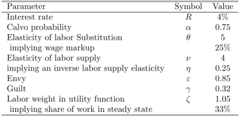
Figure 1: Relation of In‡ation to Real Variables
4
Results
Figure 1 presents the Phillips curve for the base calibration given in Table 1. On the vertical axis we show the deviations of aggregate employment and output from their respective values at the zero in‡ation steady state. The horizontal axis measures the steady state in‡ation rate.18 This …gure implies that
mone-tary policy has substantial long-run real e¤ects. Expansionary monemone-tary policy that raises in‡ation from = 0%to = 2%is associated with an increase in aggregate employment by 1:40 percent and in aggregate output by 1:32 per-cent. (As we will show in Section 4.2, the positive relation between in‡ation and macroeconomic activity is almost entirely driven by the in‡uence of envy and guilt.) The expansionary e¤ect of monetary policy declines as the in‡ation rate rises. For in‡ation rates above around = 2:25%, further increases in the rate of money growth lead to reduced aggregate employment and output.
4.1
Intuition
In our analysis, there are four channels whereby monetary policy a¤ects output and employment in the long run.
1. The employment cycling e¤ect: When in‡ation is positive, the real wage falls over the contract period (since the nominal wage is constant over the contract period while the price level rises). Under Calvo wage stagger-ing, di¤erent workers reset their nominal wages at di¤erent times. For those workers that have recently reset their nominal wages, the real wage is relatively high; whereas those workers that have not done so, the real
1 8From Ascari (2004), Amano et. al (2007), and Bakhshi et. al (2007), we know that the
Calvo staggering scheme is inadequate for steady state in‡ation rates exceeding 5%. Therefore, we restrict ourselves to in‡ation rates up to 5%.
wage is relatively low. In short, in‡ation is accompanied by ‡uctuations of relative wages. These ‡uctuations lead to ‡uctuations in relative employ-ment rates across workers, as …rms substitute cheap labor for expensive labor. Since di¤erent workers are imperfect substitutes in production, this substitution is ine¢ cient. The greater is the in‡ation rate, the greater is the amount of labor substitution and, due to the resulting ine¢ ciency, the lower is aggregate output. In short, employment cycling implies an inverse relation between in‡ation and macroeconomic activity.
2. The labor smoothing e¤ect: The greater the in‡ation rate, the more the worker’s labor supply varies over the cycle. Workers dislike variable labor supply trajectories, since their marginal disutility of labor rises with labor supplied. Thus a rise in in‡ation leads to a rise in the average real reser-vation wage over the contract period and thereby to a fall in employment and output. So labor smoothing also yields an inverse relation between in‡ation and macroeconomic activity.
3. The envy-guilt e¤ect: Workers experience relatively low incomes early in the contract period and relatively high incomes later.19 Thus they
experi-ence envy early on. To reduce their disutility from envy, they reduce their average wage so as to increase their average employment. Conversely, they experience guilt later in the contract period, leading them to re-duce average employment. But since envy is stronger than guilt, average employment rises. The greater is the in‡ation rate, the greater is the as-sociated employment and output. Thereby the envy-guilt e¤ect generates a positive relation between in‡ation and macroeconomic activity.
4. The discounting e¤ect: As noted, at the beginning of the contract period the worker’s real wage is relatively high and his employment is relatively low, and conversely later on. The worker has a constant rate of time pref-erence, and thus future utilities are discounted more heavily than present utilities. So the relatively high marginal disutilities of work occuring late in the contract period are discounted more heavily than the relatively low marginal disutilities of work occuring earlier. Accordingly, the discount-ing e¤ect leads households to supply more labor. Furthermore, guilt (felt late in the contract period) is more heavily a¤ected by discounting than envy (felt early in the contract period). Since guilt reduces labor supply while envy stimulates it, the discounting e¤ect leads to a further increase in labor supply.
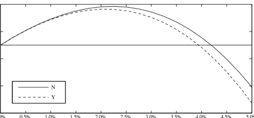
Needless to say, the latter discounting e¤ect is complementary with the envy-guilt e¤ect. This complementarity is illustrated in Figure 2, where the upper two Phillips curves portray the relation between in‡ation (on the horizontal axis)
1 9Since workers are monopolistic competitors in the labor market, the elasticity of labor
demand is greater than unity at the utility-maximizing employment level. Thus the relatively high real wages early in the contract period are associated with relatively low wage incomes.
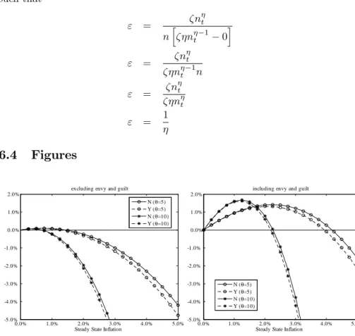
0.0% 0.5% 1.0% 1.5% 2.0% 2.5% 3.0% 3.5% 4.0% 4.5% 5.0% -5.0% -4.0% -3.0% -2.0% -1.0% 0.0% 1.0% 2.0%
Steady State Inflation N (R t=4%) Y (R t=4%) N (R t=0%) Y (Rt=0%)
Figure 2: The Complementarity between the Discounting and Envy-Guilt Ef-fects
and employment and output (on the vertical axis) in the presence of both the dis-counting and envy-guilt e¤ects (as well as the other e¤ects above), whereas the lower two Phillips curves portray this relation in the absence of the discounting e¤ect. The vertical di¤erence measures the size of the complementarity between the discounting e¤ect and the envy-guilt e¤ect (with respect to employment and output).
4.2
Sensitivities
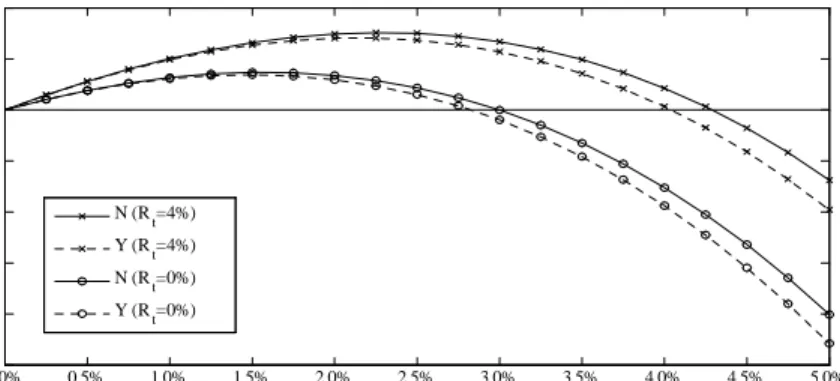
Figure 3 shows the sensitivity of the Phillips curve with respect to a range of values for the envy and guilt parameters that have been found in the literature. Holding egocentric bias constant ( , representing the relation between envy and guilt:" = ), the left panel of Figure 3 shows the Phillips curve for the following values of guilt parameter: 2 (0:24; 0:32; 0:39). Whereas our base case is = 0:32, the value = 0:24was supported by Fehr and Schmidt (2003) and the value = 0:39was found by Goeree and Holt (2000).20 Figure 3 shows,
not surprisingly, that when the guilt and envy e¤ects strengthen the positive long-run e¤ect of monetary policy on output and employment increases.
The right panel of Figure 3 indicates that this positive e¤ect rises with the degree of egocentric bias, i.e. the greater the envy associated with any given level of guilt, the more monetary policy stimulates output and employment in the long run. This result is also not surprising in the light of the analysis above. The …gure shows the Phillips curve for the following values of the egocentric
2 0Goeree and Holt (2000) estimate the Fehr and Schmidt paramters with experimental data
from a two stage-ultimatum game. Support for their estimates comes from Blanco et al. (2011), who apply the same estimation methodology but resort to observations obtained from utlimatum games, dictator games, public goods games, and prisoner’s dilemma games. They …nd the value = 0:38.
0.0% 1.0% 2.0% 3.0% 4.0% 5.0% -3.0% -2.0% -1.0% 0.0% 1.0% 2.0%
Steady State Inflation
0.0% 1.0% 2.0% 3.0% 4.0% 5.0% -6.0% -4.0% -2.0% 0.0% 2.0% 4.0% 6.0%
Steady State Inflation N (γ=0.24) Y (γ=0.24) N (γ=0.32) Y (γ=0.32) N (γ=0.39) Y (γ=0.39) N (κ=1) Y (κ=1) N (κ=2.7) Y (κ=2.7) N (κ=3.5) Y (κ=3.5) N (κ=5.1) Y (κ=5.1)
Figure 3: Sensitivity with respect to guilt parameters
bias parameter: 2(1; 2:7; 3:5; 5:1), where our base case is = 2:7. With the exception of = 1, all values of the parameters were found in Loewenstein at al. (1989). In particular, while = 2:7was found for a neutral relationship be-tween the judging subject and her reference subject, Loewenstein et al. (1989) …nd that = 3:5 and = 5:1 to apply to positive and negative relationship environments, respectively. Moreover, to highlight the importance of the ego-centric bias, Figure 3 also displays the results for = 1, i.e. in the abscence of any egocentric bias. In this case, the envy and guilt e¤ects play a negligible role and therefore, monetary policy has no substantial positive implications for long-run output and employment. This result holds irrespective of the value of
.
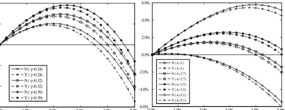
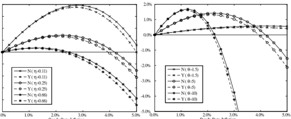
Figure 4 shows the sensitivity of the Phillips curve with respect to reasonable values for the labor supply and labor substitution elasticities = 1 and . The left panel of Figure 4 juxtaposes Phillips curves for the labor supply elasticities
2(1:5; 4; 9), where our base case is = 4 ( = 0:25). The higher labor supply
elasticitiy = 9 ( = 0:11)was estimated by Abowd and Card (1989) and the lower value = 1:5 ( = 0:66)was found by Mulligan (1998) and Heckman et al. (1998). The latter is very close to the values chosen by Rotemberg and Woodford (1996) and Hansen and Wright (1992) in their theoretical contributions. As is apparent from the left panel of Figure 4, the lower the labor supply elasticity (i.e. the higher ), the smaller the e¤ectiveness of monetary policy with respect to aggregate employment and output. Intuitively, the greater the convexity of utility with respect to labor, the more aversive are households to a non-smooth path of labor supply and therefore, the stronger is the labor non-smoothing e¤ect.21 As discussed above, the labor smoothing e¤ect raises the average real
reservation wage, thereby reducing employment and output. Consequently, the Phillips curve shifts downwards.
0.0% 1.0% 2.0% 3.0% 4.0% 5.0% -5.0% -4.0% -3.0% -2.0% -1.0% 0.0% 1.0% 2.0% 3.0% 4.0%
Steady State Inflation 0.0% 1.0% 2.0% 3.0% 4.0% 5.0% -5.0% -4.0% -3.0% -2.0% -1.0% 0.0% 1.0% 2.0%
Steady State Inflation N (η=0.11) Y (η=0.11) N (η=0.25) Y (η=0.25) N (η=0.66) Y (η=0.66) N (θ=1.5) Y (θ=1.5) N (θ=5) Y (θ=5) N (θ=10) Y (θ=10)
Figure 4: Sensitivity with respect to elasticities
The right panel of Figure 4 shows how the long-run Phillips curve is a¤ected by the degree of labor substitutability over the interval 2 (1:5; 5; 10). The higher the value , the more substitutable are the labor types. We contrast our base case = 5with a very low degree of substitutability = 1:5 as estimated by Ciccone and Peri (2005) and a high degree of substitutability = 10 as found in Fagan and Messina (2009).22 As the right panel of Figure 4 indicates,
the more substitutable labor types are, the greater the real e¤ects of monetary policy, but over a narrower range. Intuitively, raising the substitutability of labor types has three e¤ects on aggregate. First, it reduces the ine¢ ciencies from labor substitution, so that for a given the amount of employment cycling, output increases. Second, labor substitution becomes cheaper, increasing the incentive for employment cycling, so that output decreases23 (ceteris paribus).
Third, the increase in employment cycling raises the dispersion of incomes, thereby eliciting more envy and guilt. Since the envy e¤ect is greater than the guilt e¤ect, aggregate output increases (ceteris paribus). As is apparent from the right panel of Figure 4, the positive e¤ects on output (particularly from the envy e¤ect)24are dominant at low in‡ation rates, whereas the negative e¤ects on output (from additional employment cycling) are dominant at higher in‡ation
. For = 0:66, increases from1:05to1:65, while it decreases to0:9025for = 0:11.
2 2On the basis on various country studies, Aidt and Tzannatos (2002) summarize that the
average wage markup in industrialized as well as in developing countries lies in the intervall between10and25%, which implies5 10. The low value found by Ciccone and Peri (2005) arises from the fact that they explicitely estimate the markup for high skilled workers over low skilled workers.
2 3Employment cycling has a direct, negative e¤ect on output, as well as an indirect, negative
e¤ect via the households’reservation wage (which rises because households’utility falls when employment cycling increases).
2 4As is apparent from Figure 6 in the appendix, the positive e¤ects of a reduction in
in-e¢ ciencies from labor substitution are quantitatively negligible (left panel). Therefore, the positive e¤ect can be almost entirely attributed to the envy e¤ect (right panel).
0.0% 1.0% 2.0% 3.0% 4.0% 5.0% -3.0% -2.0% -1.0% 0.0% 1.0% 2.0%
Steady State Inflation N (α=0.66) Y (α=0.66) N (α=0.75) Y (α=0.75) N (α=0.82) Y (α=0.82)
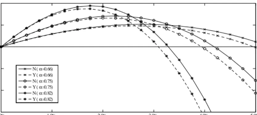
Figure 5: Figure 5: Sensitivity with respect to wage stickiness
rates.
Figure 5 shows the the Phillips curve for di¤erent wage stickiness parameters over the range 2(0:66; 0:75; 0:88). While in our base calibration wages change on average once a year( = 0:75), Barattieri et al. (2010) …nd wages to be a little less ‡exible, i.e. wages change on average every six quarters( = 0:82). Christiano et al. (2005) estimate wages to be sticky for approximately half a
year( = 0:66). Analogously to the previous …gure, Figure 5 indicates that the
stickier wages are, the more e¤ective is monetary policy, but over a narrower range. Intuitively, the stickier wages are, the larger is real wage dispersion and thus the larger is real income dispersion. Consequently, there is more envy and guilt, and since the envy e¤ect is strong, output increases. On the other hand, a larger real wage dispersion implies more labor substitution, which promotes the employment cycling and thereby reduces output. The envy e¤ect dominates at low in‡ation rates, whereas the employment cycling e¤ects dominates at high in‡ation rates.
5
Optimal Monetary Policy
In the long run, the optimal rate of money growth (equal to the optimal in‡ation rate) maximizes the lifetime utility of the representative household:
max 1+ U = 1 X i=0 ( )i " cj;t+i n1+j;t+i 1 + j;t+i Ij;t2+i 2 # (15)
subject to the labor demand contraint (2), the labor supply constraint (8), and the reset wage (14).
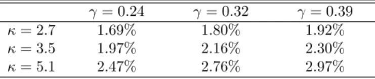
The following table presents the optimal in‡ation rates for our base calibra-tion, as well as for other values of the envy-guilt parameters. Recalling that in
= 0:24 = 0:32 = 0:39 = 2:7 1.69% 1.80% 1.92%
= 3:5 1.97% 2.16% 2.30%
= 5:1 2.47% 2.76% 2.97% Table 2: Welfare with respect to envy and guilt
the base case = 2:7 and = 0:32, we …nd that optimal in‡ation is slightly below 2 percent in our base calibration. The higher value of the guilt parameter (with constant egocentric bias) implies a slightly higher optimal in‡ation rate, and conversely for a lower value of the guilt parameter. Furthermore, greater egocentric bias (with a constant guilt parameter) implies higher optimal in‡a-tion, and conversely for less egocentric bias.
The intuition underlying these results is straightforward. The optimal in‡ation rate is positive for two reasons: (1) When the in‡ation rate is zero, output and employment are ine¢ ciently low, since workers are monopolistic competitors in the labor market. (2) Due to the envy-guilt and discounting e¤ects, higher in‡ation is associated with greater output and employment, over a range of low in‡ation rates. On this account, a positive long-run rate of money growth is able to reduce the ine¢ ciency from monopolistic competition.
More precisely, when the money growth rate rises above zero, it a¤ects wel-fare in the following ways: (1) it reduces the ine¢ ciency from monopolistic competition and thereby raises the utility from consumption, (2) it raises the ine¢ ciency from employment cycling, (3) it increases the disutility of labor due to a more volatile labor trajectory and (4) it increases the disutility from envy and guilt. While the …rst in‡uence enters the utility function linearly in out-put, the other in‡uences grow exponentially as in‡ation increases output and employment. Thus the …rst in‡uence dominates at low in‡ation rates, whereas the latter in‡uences dominate at higher in‡ation rates.
Needless to say, the ine¢ ciency from monopolistic competition can be re-duced in ways other than expansionary monetary policy and these other ways may have more favorable welfare e¤ects than expansionary monetary policy. But the overarching implication of our analysis is this. If, for whatever rea-son,25 the equilibrium levels of output and employment are ine¢ ciently low –
after the government has implemented all its …scal and structural policies – then expansionary monetary policy can be welfare-promoting by reducing the residual ine¢ ciency.
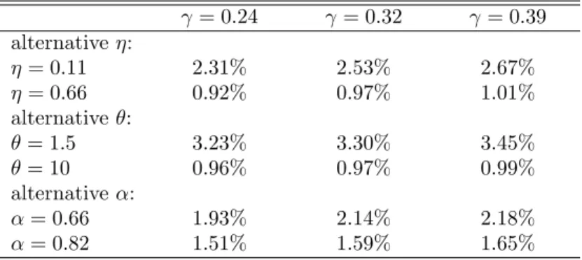
shows how the optimal in‡ation rate varies with respect to di¤erent values26 for the intertemporal and intratemporal labor substitution elasticities and ;
respectively, and the degree of wage stickiness .
Table 3The …rst two rows of Table 3 indicate that the optimal in‡ation rate is negatively related to the inverse of the labor supply elasticity = 1.
2 5There are of course many conceivable reasons why output and employment may be too
low, such as distortionary taxes, e¢ ciency-wage, insider-outsider, or union-power e¤ects.
= 0:24 = 0:32 = 0:39 alternative : = 0:11 2.31% 2.53% 2.67% = 0:66 0.92% 0.97% 1.01% alternative : = 1:5 3.23% 3.30% 3.45% = 10 0.96% 0.97% 0.99% alternative : = 0:66 1.93% 2.14% 2.18% = 0:82 1.51% 1.59% 1.65% Table 3: Welfare with respect to model parameters
Intuitively, when the convexity of utility with respect to labor rises, the disutility of work increases relative to the utility of consumption. Since the bene…ts of extra output decline more rapidly, reducing the optimal in‡ation rate.
The next two rows of Table 3 show that the greater the substitutability among labor types, the lower is the optimal in‡ation rate. The degree of substi-tutability measures the market power of the di¤erent worker types. The lower , the higher is the market power of each labor type, and thus the larger is the ine¢ ciency from monopolistic competition, implying a lower optimal in‡ation rate.
Finally, the last two rows of Table 3 indicate that the greater is the degree of wage stickiness, the lower is the optimal in‡ation rate. Intuitively, the greater is the degree of wage stickiness the more dispersed is the real wage distribution and the greater is employment cycling. This reduces utility due to the ine¢ ciency of employment cycling, households’ aversion to volatile incomes, and the envy and guilt e¤ects. Thus the optimal in‡ation rate falls.
6
Conclusion
We have shown that, in the presence of staggered, monopolistically competi-tive nominal wage contracts, inequity aversion can generate a posicompeti-tive long-run tradeo¤ between in‡ation and macroeconomic activity. Under these circum-stances, our analysis implies that expansionary monetary policy – leading to a low, positive in‡ation rate – is socially optimal. For our base calibration, the optimal in‡ation rate is just under 2 percent.
Our analysis is meant to help bridge the gap between monetary theory and central banking practice. In contrast to much of the recent literature on mon-etary policy, we provide a rationale for targeting in‡ation at a low, positive rate.
In our analysis, the relation between in‡ation and macroeconomic activity is the outcome of four phenomena: employment cycling, labor supply variability, discounting and envy-guilt e¤ects. The …rst two phenomena imply an inverse
relation between in‡ation and macroeconomic activity, whereas the last two are complementary and imply a positive relation. Furthermore, the last two dominate at low in‡ation rates, whereas the …rst two dominate at high in‡ation rates. Consequently, the Phillips curve is backward-bending, so that increases in money growth lead to higher employment and output at low in‡ation, but to lower employment and output at high in‡ation.
In this context, the role of optimal monetary policy is to reduce ine¢ cien-cies that generate suboptimally low employment and output. This provides a rationale for a low, positive long-run in‡ation target.
References
Abowd, J. M. and D. Card (1989). On the covariance structure of earnings and hours changes.Econometrica 57(2), 411–445.
Adams, J. S. (1965). Inequity in social exchange. InAdvance in Experimental Psychology, Volume 2, pp. 267–299. New York: Academic Press.
Ahmed, S. and J. H. Rogers (1998). In‡ation and the great ratios: long-term evidence from the U.S. International Finance Discussion Papers 628, Board of Governors of the Federal Reserve System (U.S.).
Aidt, T. and Z. Tzannatos (2002). Unions and Collective Bargaining: Eco-nomic E¤ ects in a Global Environment. The World Bank, Washington D.C.
Akerlof, G. A., W. R. Dickens, and G. L. Perry (1996). The macroeconomics of low in‡ation.Brookings Papers on Economic Activity 27(1996-1), 1–76. Akerlof, G. A. and W. T. Dickens (2007). Un…nished business in the macroeco-nomics of low in‡ation: A tribute to George and Bill by Bill and George.
Brookings Papers on Economic Activity 38(2007-2), 31–48.
Akerlof, G. A., W. T. Dickens, and G. L. Perry (2000). Near-rational wage and price setting and the long-run phillips curve. Brookings Papers on Economic Activity 31(2000-1), 1–60.
Amano, R., S. Ambler, and N. Rebei (2007). The macroeconomic e¤ects of nonzero trend in‡ation. Journal of Money, Credit and Banking 39(7), 1821–1838.
Argyle, M. (1972).The Social Psychology of Work. Tablinger Publishing Com-pany, New York.
Argyle, M. (1989).The Psychology of Happiness. Routledge, London. Aruoba, S. B. and F. Schorfheide (2011). Sticky prices versus monetary
fric-tions: An estimation of policy trade-o¤s. American Economic Journal: Macroeconomics 3(1), 60–90.
Ascari, G. (1998). Superneutrality of money in staggered wage-setting models.
Ascari, G. (2000). Optimising agents, staggered wages and persistence in the real e¤ects of money shocks.Economic Journal 110(465), 664–686. Ascari, G. (2004). Staggered prices and trend in‡ation: Some nuisances.
Re-view of Economic Dynamics 7(3), 642–667.
Ascari, G. and C. Merkl (2009). Real wage rigidities and the cost of disin‡a-tions.Journal of Money, Credit and Banking 41(2-3), 417–435.
Bae, S.-K. and R. A. Ratti (2000). Long-run neutrality, high in‡ation, and bank insolvencies in Argentina and Brazil. Journal of Monetary Eco-nomics 46(3), 581–604.
Bakhshi, H., H. Khan, P. Burriel-Llombart, and B. Rudolf (2007). The new keynesian phillips curve under trend in‡ation and strategic complemen-tarity.Journal of Macroeconomics 29(1), 37–59.
Ball, L. (1997). Disin‡ation and the NAIRU. In C. D. Romer and D. H. Romer (Eds.),Reducing In‡ation: Motivation and Strategy. University of Chicago Press.
Ball, L. (1999). Aggregate demand and long-term unemployment. Brookings Papers on Economic Activity 30(2), 189–252.
Barattieri, A., S. Basu, and P. Gottschalk (2010). Some evidence on the im-portance of sticky wages. NBER Working Papers 16130, National Bureau of Economic Research, Inc.
Benabou, R. and J. D. Konieczny (1994). On in‡ation and output with costly price changes: A simple unifying result. American Economic Re-view 84(1), 290–297.
Berentsen, A., G. Menzio, and R. Wright (2011). In‡ation and unemployment in the long run.American Economic Review 101(1), 371–98.
Beyer, A. and R. E. Farmer (2007). Natural rate doubts.Journal of Economic Dynamics and Control 31(3), 797–825.
Blanch‡ower, D. G. and A. J. Oswald (2004). Well-being over time in Britain and the USA.Journal of Public Economics 88(7-8), 1359–1386.
Blanco, M., D. Engelmann, and H.-T. Normann (2011). A within-subject analysis of other-regarding preferences. Games and Economic Behav-ior 72(2), 321–338.
Blundell, R. and T. Macurdy (1999). Labor supply: A review of alternative approaches. In O. Ashenfelter and D. Card (Eds.), Handbook of Labor Economics, Volume 3 ofHandbook of Labor Economics, Chapter 27, pp. 1559–1695. Elsevier.
Bolton, G. E. and A. Ockenfels (2000). ERC: A theory of equity, reciprocity, and competition.American Economic Review 90(1), 166–193.
Bullard, J. and J. W. Keating (1995). The long-run relationship between in‡ation and output in postwar economies. Journal of Monetary Eco-nomics 36(3), 477–496.
Calvo, G. A. (1983). Staggered prices in a utility-maximizing framework.
Journal of Monetary Economics 12(3), 383–398.
Camerer, C. F., G. F. Loewenstein, and D. Prelec (2005). Neuroeconomics: How neuroscience can inform economics. Journal of Economic Litera-ture 43(1), 9–64.
Cappelen, A. W., K. Nygaard, E. Sörensen, and B. Tungodden (2010, Novem-ber). E¢ ciency, equality and reciprocity in social preferences: A compar-ison of students and a representative population. Discussion Paper Series in Economics 28/2010, Department of Economics, Norwegian School of Economics.
Cappelen, A. W., K. Nygaard, E. Sörensen, and B. Tungodden (2011). Social preferences in the lab: A comparison of students and a representative population. CESifo Working Paper Series 3511, CESifo Group Munich. Carare, A. and M. R. Stone (2006). In‡ation targeting regimes. European
Economic Review 50(5), 1297–1315.
Chen, S.-W. (2007). Evidence of the long-run neutrality of money: The case of South Korea and Taiwan.Economics Bulletin 3(64), 1–18.
Christiano, L. J., M. Eichenbaum, and C. L. Evans (2005). Nominal rigidities and the dynamic e¤ects of a shock to monetary policy.Journal of Political Economy 113(1), 1–45.
Ciccone, A. and G. Peri (2005). Long-run substitutability between more and less educated workers: Evidence from U.S. states, 1950-1990.The Review of Economics and Statistics 87(4), 652–663.
Clark, A. E., P. Frijters, and M. A. Shields (2008). Relative income, happiness, and utility: An explanation for the easterlin paradox and other puzzles.
Journal of Economic Literature 46(1), 95–144.
Clark, A. E. and A. J. Oswald (1996). Satisfaction and comparison income.
Journal of Public Economics 61(3), 359–381.
Coenen, G., A. Orphanides, and V. Wieland (2004). Price stability and mon-etary policy e¤ectiveness when nominal interest rates are bounded at zero.
The B.E. Journal of Macroeconomics 0(1).
Coibion, O., Y. Gorodnichenko, and J. F. Wieland (2010, June). The optimal in‡ation rate in new keynesian models. NBER Working Papers 16093, National Bureau of Economic Research, Inc.
Dixit, A. K. and J. E. Stiglitz (1977). Monopolistic competition and optimum product diversity.American Economic Review 67(3), 297–308.
Dolado, J. J., J. D. López-Salido, and J. L. Vega (2000). Unemployment and in‡ation persistence in Spain: Are there phillips trade-o¤s? Spanish Economic Review 2(3), 267–291.
Domeij, D. and M. Floden (2006). The labor-supply elasticity and borrow-ing constraints: Why estimates are biased. Review of Economic Dynam-ics 9(2), 242–262.
Easterlin, R. A. (1974). Does economic growth improve the human lot? some empirical evidence. In P. A. David and M. W. Reder (Eds.),Nations and Households in Economic Growth: Essays in Honor of Moses Abramovitz. New York: Academic Press.
Easterlin, R. A. (1995). Will raising the incomes of all increase the happiness of all? Journal of Economic Behavior & Organization 27(1), 35–47. Erceg, C. J., D. W. Henderson, and A. T. Levin (2000). Optimal monetary
policy with staggered wage and price contracts.Journal of Monetary Eco-nomics 46(2), 281–313.
Ericsson, N. R., J. S. Irons, and R. W. Tryon (2001). Output and in‡ation in the long run.Journal of Applied Econometrics 16(3), 241–253.
Fagan, G. and J. Messina (2009). Downward wage rigidity and optimal steady-state in‡ation. Working Paper Series 1048, European Central Bank. Fair, R. C. (2000). Testing the nairu model for the United States.The Review
of Economics and Statistics 82(1), 64–71.
Favara, G. and P. Giordani (2009). Reconsidering the role of money for out-put, prices and interest rates.Journal of Monetary Economics 56(3), 419– 430.
Fehr, E. and K. Schmidt (2003). Theories of fairness and reciprocity – evi-dence and economic applications. In M. Dewatripont, L. P. Hansen, and S. J. Turnovsky (Eds.),Advances in Economics, Volume 1, pp. 208–257. Econometric Society Monographs,Eight World Congress.
Fehr, E. and K. M. Schmidt (1999). A theory of fairness, competition, and cooperation.The Quarterly Journal of Economics 114(3), 817–868. Fisher, M. E. and J. J. Seater (1993). Long-run neutrality and superneutrality
in an arima framework.American Economic Review 83(3), 402–415. Forsythe, R., J. L. Horowitz, N. E. Savin, and M. Sefton (1994). Fairness
in simple bargaining experiments. Games and Economic Behavior 6(3), 347–369.
Galí, J. (2003). New perspectives on monetary policy, in‡ation, and the busi-ness cycle. In L. H. M. Dewatripont and S. Turnovsky (Eds.),Advances in Economic Theory, Volume 3, pp. 151–197. Cambridge University Press. Galí, J., F. Smets, and R. Wouters (2011). Unemployment in an estimated
new keynesian model. In NBER Macroeconomics Annual 2011, Volume 26, NBER Chapters. National Bureau of Economic Research, Inc. Goeree, J. K. and C. A. Holt (2000). Asymmetric inequality aversion and
noisy behavior in alternating-o¤er bargaining games.European Economic Review 44(4-6), 1079–1089.
Gottschalk, J. and U. Fritsche (2005). The new keynesian model and the long-run vertical phillips curve: Does it hold for Germany? Discussion Papers of DIW Berlin 521, DIW Berlin, German Institute for Economic Research.
Graham, L. and D. J. Snower (2004). The real e¤ects of money growth in dynamic general equilibrium. Working Paper Series 412, European Central Bank.
Graham, L. and D. J. Snower (2008). Hyperbolic discounting and the phillips curve.Journal of Money, Credit and Banking 40(2-3), 427–448.
Graham, L. and D. J. Snower (2011, May). Hyperbolic discounting and posi-tive optimal in‡ation. CEPR Discussion Papers 8390, C.E.P.R. Discussion Papers.
Güth, W., R. Schmittberger, and B. Schwarze (1982). An experimental analy-sis of ultimatum bargaining.Journal of Economic Behavior & Organiza-tion 3(4), 367–388.
Hansen, G. D. and R. Wright (1992). The labor market in real business cycle theory.Quarterly Review, 2–12.
Heckman, J., L. Lochner, and C. Taber (1998). Explaining rising wage in-equality: Explanations with a dynamic general equilibrium model of labor earnings with heterogeneous agents.Review of Economic Dynamics 1(1), 1–58.
Henrich, J., R. Boyd, S. Bowles, C. Camerer, E. Fehr, H. Gintis, and R. McEl-reath (2001). In search of homo economicus: Behavioral experiments in 15 small-scale societies.American Economic Review 91(2), 73–78. Homans, G. C. (1961). Social behavior: its elementary forms. New York :
Harcourt, Brace & World.
Imai, S. and M. P. Keane (2004). Intertemporal labor supply and human capital accumulation.International Economic Review 45(2), 601–641. Jaques, E. (1956).Measurement of Responsibility. A Study of Work, Payment,
and Individual Capacity. London: Tavistock Publications.
Jaques, E. (1961). Equitable payment: a general theory of work, di¤ erential payment, and individual progress. London: Heinemann.
Kapteyn, A. and F. G. Van Herwaarden (1980). Interdependent welfare func-tions and optimal income distribution.Journal of Public Economics 14(3), 375–397.
Karanassou, M. and H. Sala (2010). The US in‡ation-unemployment trade-o¤ revisited: New evidence for policy-making. Journal of Policy Model-ing 32(6), 758–777.
Karanassou, M., H. Sala, and D. J. Snower (2003). The European phillips curve: Does the NAIRU exist? Applied Economics Quarterly 2(876), 93– 121.
Karanassou, M., H. Sala, and D. J. Snower (2005). A reappraisal of the in‡ation-unemployment tradeo¤. European Journal of Political Econ-omy 21(1), 1–32.
Karanassou, M., H. Sala, and D. J. Snower (2008). The evolution of in‡ation and unemployment: Explaining the roaring nineties.Australian Economic Papers 47(4), 334–354.
Karni, E. and Z. Safra (2002). Individual sense of justice: A utility represen-tation.Econometrica 70(1), 263–284.
Karni, E., T. Salmon, and B. Sopher (2008). Individual sense of fairness: an experimental study.Experimental Economics 11(2), 174–189.
Khan, A., R. G. King, and A. L. Wolman (2003). Optimal monetary policy.
Review of Economic Studies 70(4), 825–860.
King, R. G. and M. W. Watson (1994). The post-war U.S. phillips curve: a revisionist econometric history.Carnegie-Rochester Conference Series on Public Policy 41(1), 157–219.
King, R. G. and A. L. Wolman (1996). In‡ation targeting in a St. Louis model of the 21st century.Proceedings, 83–107.
Konieczny, J. D. (1990). In‡ation, output and labour productivity when prices are changed infrequently.Economica 57(226), 201–218.
Koustas, Z. (1998). Canadian evidence on long-run neutrality propositions.
Journal of Macroeconomics 20(2), 397–411.
Koustas, Z. and A. Serletis (2003). Long-run phillips-type trade-o¤s in Euro-pean Union countries.Economic Modelling 20(4), 679–701.
Koustas, Z. and W. Veloce (1996). Unemployment hysteresis in Canada: An approach based on long-memory time series models. Applied Eco-nomics 28(7), 823–831.
Kuran, T. (1986). Price adjustment costs, anticipated in‡ation, and output.
The Quarterly Journal of Economics 101(2), 407–418.
Layard, R., G. Mayraz, and S. Nickell (2009). Does relative income matter? are the critics right? CEP Discussion Papers dp0918, Centre for Economic Performance, LSE.
Loewenstein, G., S. Rick, and J. D. Cohen (2008). Neuroeconomics. Annual Review of Psychology 59, 647–672.
Loewenstein, G. F., L. Thompson, and M. H. Bazerman (1989). Social utility and decision making in interpersonal contexts.Journal of Personality & Social Psychology 57(3), 426–441.
Mankiw, N. G. (2001). The inexorable and mysterious tradeo¤ between in‡a-tion and unemployment.Economic Journal 111(471), C45–61.
Messick, D. M. and K. P. Sentis (1979). Fairness and preferences.Journal of Experimental Social Psychology 15(4), 418–434.
Messick, D. M. and K. P. Sentis (1985). Estimating social and nonsocial utility functions from ordinal data.European Journal of Social Psychology 15(4), 389–399.
Mulligan, C. B. (1999). Substition over time: Another look at life-cycle la-bor supply. In NBER Macroeconomics Annual 1998, volume 13, NBER Chapters, pp. 75–152. National Bureau of Economic Research, Inc. Naish, H. F. (1986). Price adjustment costs and the output-in‡ation trade-o¤.
Economica 53(210), 219–230.
Nelson, E. (2007). Comment on: Samuel Reynard’s "maintaining low in-‡ation: Money, interest rates, and policy stance". Journal of Monetary Economics 54(5), 1472–1479.
Nelson, E. (2008). Why money growth determines in‡ation in the long run: Answering the woodford critique. Journal of Money, Credit and Bank-ing 40(8), 1791–1814.
Orphanides, A. and R. M. Solow (1990). Money, in‡ation and growth. In B. M. Friedman and F. H. Hahn (Eds.),Handbook of Monetary Economics, Volume 1 of Handbook of Monetary Economics, Chapter 6, pp. 223–261. Elsevier.
Puah, C.-H., M. S. Habibullah, and S. A. Mansor (2008). On the long-run monetary neutrality: Evidence from the SEACEN countries. Journal of Money, Investment and Banking 2, 50–62.
Ransom, M. R. and D. P. Sims (2010). Estimating the …rm’s labor supply curve in a new monopsony framework: Schoolteachers in Missouri.Journal of Labor Economics 28(2), 331–355.
Reynard, S. (2007). Maintaining low in‡ation: Money, interest rates, and policy stance.Journal of Monetary Economics 54(5), 1441–1471. Roger, S. and M. R. Stone (2005). On target? the international experience
with achieving in‡ation targets. IMF Working Papers 05/163, Interna-tional Monetary Fund.
Rotemberg, J. J. and M. Woodford (1996). Real-business-cycle models and the forecastable movements in output, hours, and consumption.American Economic Review 86(1), 71–89.
Roth, A. E., V. Prasnikar, M. Okuno-Fujiwara, and S. Zamir (1991). Bargain-ing and market behavior in Jerusalem, Ljubljana, Pittsburgh, and Tokyo: An experimental study.American Economic Review 81(5), 1068–1095. Russell, B. and A. Banerjee (2008). The long-run phillips curve and
non-stationary in‡ation.Journal of Macroeconomics 30(4), 1792–1815. Sanfey, A. G., J. K. Rilling, J. A. Aronson, L. E. Nystrom, and J. D. Cohen
(2003). The neural basis of economic decision-making in the ultimatum game.Science 300(5626), 1755 –1758.
Schmitt-Grohé, S. and M. Uribe (2007). Optimal in‡ation stabilization in a medium-scale macroeconomic model. In F. S. Miskin, K. Schmidt-Hebbel, N. L. S. Editor), and K. S.-H. (Se (Eds.), Monetary Policy under In‡a-tion Targeting, Volume 11 of Central Banking, Analysis, and Economic Policies Book Series, Chapter 5, pp. 125–186. Central Bank of Chile.
Schmitt-Grohé, S. and M. Uribe (2010). The optimal rate of in‡ation. NBER Working Papers 16054, National Bureau of Economic Research, Inc. Schreiber, S. and J. Wolters (2007). The long-run phillips curve
revis-ited: Is the NAIRU framework data-consistent? Journal of Macroeco-nomics 29(2), 355–367.
Scitovsky, T. (1992). The Joyless Economy: The Psychology of Human Sat-isfaction. New York: Oxford University Press.
Solnick, S. J. and D. Hemenway (1998). Is more always better?: A survey on positional concerns.Journal of Economic Behavior & Organization 37(3), 373–383.
Taylor, J. B. (1979). Staggered wage setting in a macro model. American Economic Review 69(2), 108–113.
Taylor, J. B. (1999). Staggered price and wage setting in macroeconomics. In J. B. Taylor and M. Woodford (Eds.), Handbook of Macroeconomics, Volume 1 of Handbook of Macroeconomics, Chapter 15, pp. 1009–1050. Elsevier.
Tversky, A. and D. Kahneman (1991). Loss aversion in riskless choice: A reference-dependent model.The Quarterly Journal of Economics 106(4), 1039–1061.
van de Stadt, H., A. Kapteyn, and S. van de Geer (1985). The relativity of utility: Evidence from panel data.The Review of Economics and Statis-tics 67(2), 179–187.
Wallace, F. H. and G. L. Shelley (2004). Long run neutrality and superneu-trality of money: Aggregate and sectoral tests for Nicaragua.EconWPA, Macroeconomics (0402004).
Wallace, F. H. and G. L. Shelley (2007). Long run neutrality of money in Mexico.Economia Mexicana NUEVA EPOCA 0(2), 219–238.
Walster, E., G. W. Walster, and E. Berscheid (1978). Equity: Theory and Research. Boston: Allyn and Bacon.
Woodford, M. (2003). Interest and Prices. Princeton: Princeton University Press.
Yun, T. (1996). Monetary policy, nominal price rigidity, and business cycles.
Journal of Monetary Economics 37, 345–370.
Yun, T. (2005). Optimal monetary policy with relative price distortions.
Appendix
6.1
Steady State Relative Wage
To calculate the steady state we drop the time indices. The detrended wage index in a Calvo world is given by
wt= " (1 )wt1 + wt 1 1 + 1 #11 (16)
In the steady state we drop time indices
w1 = (1 )w 1 + w 1 + 1 (17) Grouping terms 1 (1 + ) 1 W1 = (1 )W 1 (18)
and re-arranging yields the optimal relative steady state wage
wj = 1 1 (1 + ) 1 ! 1 1 : (19)
6.2
Wage dispersion
From aggregate labor and the individual labor demand we get
nt = Z 1 0 wk;tytdk; (20) nt = yt Z 1 0 wk;tdk | {z } st ; (21) nt = styt: (22) Furthermore st = Z 1 0 wk;tdk; (23) = (1 )wk;t+ (1 ) wk;t 1 (1 + ) 1 + 2(1 ) wk;t 2 (1 + ) 2 +: : : ;(24) = (1 )wk;t+ (1 + ) " (1 )wk;t 1+ (1 ) wk;t 2 (1 + ) 1 +: : : # ; (25) = (1 )wk;t+ (1 + ) st 1 (26)
which in the steady state is given by
s = (1 )wk + (1 + ) s; (27)
s = (1 )wk
1 (1 + ) : (28)
Derivation of Labor Supply Curve
The worker maximizes utility
max wj;t Et 1 X i=0 ( )i U cj;t+i V nj;t+i Z Ij;t+i (29)
subject to its budget constraint
cj;t+i+mj;t+1+i+bj;t+1+i = (30)
wj;t
(1 + )inj;t+i+
Rt+ibj;t+i+mj;t+i
1 + + j;t+1+i:
wheremandbare real money and bond holdings and are lump sum transfers from the government to workers and the downward-sloping labor demand
nj;t+i=
wj;t
(1 + )i
!
yt+i (31)
and inequity aversion
Ij;t+i = wj;t (1 + )inj;t+i Z 1 0 wk;t+ink;t+idk | {z } N ; (32)
whereN denotes the average income in the economy. The …rst order condition of this maximization problem yields
Et 1 X i=0 ( )i (1 )Uc nj;t+i (1 + )i + Vn nj;t+i wj;t (1 )ZI nj;t+i (1 + )i = 0: (33)
Re-arranging equation (33) we get
Et 1 X i=0 ( )i Vn nj;t+i wj;t (34) = ( 1) " Et 1 X i=0 ( )iUcnj;t+i (1 + )i Et 1 X i=0 ( )i ZInj;t+i (1 + )i # :
Rearranging equation (34) with respect towj;t yields
wj;t= 1 EtP1i=0( ) i Vnnj;t+i EtP1i=0( ) i Uc(1+ )nj;t+ii EtP1i=0( ) i ZInj;t+i (1+ )i : (35)
From the utility function U(cj; nj;Ij) =cj;t n1+j;t 1 + j;t I2 j;t 2 (36)
we obtain the …rst order conditionsVn,Uc, andZI:
Vn = nj;t+i; (37)
Uc = 1; (38)
ZI = j;t+iIj;t+i (39)
Plugging equations (37), (38), and (39) into (35) gives the optimal reset wage as in Section 3.2 wj;t= w Et P1 i=0( ) i n1+j;t+i EtP1i=0( )i n(1+ )j;t+ii Et P1 i=0( ) i j;t+iIj;t+i(1+ )nj;t+ii : (40)
where w= 1 denotes the markup. This is equation (8) in Section 3. Rear-ranging equation (40) yields the labor supply equation (9)
1 w = EtP1i=0( ) i n1+j;t+i EtP1i=0( ) i wj;tnj;t+i (1+ )i EtP1i=0( ) i j;t+iIj;t+i wj;tnj;t+i (1+ )i : (41)
Note that envy and guilt needs to be considered separately, i.e. the term to the right in the denominator is de…ned as
Et 1 X i=0 ( )i j;t+iIj;t+i wj;tnj;t+i (1 + )i = (42) "Et 1 X i=0 ( )iIj;t+i wj;tnj;t+i (1 + )i + Et 1 X i= ( )iIj;t+i wj;tnj;t+i (1 + )i
where denotes the threshold at which the worker exceeds the average income in the economy and j;tis an indicator function, which takes values
j;t=
" for Ij;t<0
for Ij;t>0 : (43)
Applying the downward sloping labor demand equation (31), we can write equa-tion (41) in terms of aggregate labor.
1 w = EtP1i=0 (1 + ) (1+ ) i wj;t(1+ )yt1++i EtP1i=0 (1 + ) ( 1) i yt+i wj;t1 EtP1i=0 (1 + )( 1) i j;t+iIj;t+iwyt+i1 j;t : (44)
Rearranging terms wj;t1+ w = EtP1i=0 (1 + ) (1+ ) i y1+t+i EtP1i=0 (1 + )( 1) i yt+i EtP1i=0 (1 + )( 1) i yt+i j;t+iIj;t+i : (45) In the steady state we drop time indices
wj1+ w =y EP1i=0 (1 + ) (1+ ) i EP1i=0 (1 + )( 1) i E 1 X i=0 (1 + )( 1) i j;iIj;i | {z } EG ; (46) In order to be able to solve the model numerically, we need to let the in…nite sums converge. The sum formulation in the numerator can be written in terms of in…nite geometric sums according to X1
k=ox
k = 1
1 x. In the case of the
denominator this is a lot more complicated. Remember that there is a kink due to envy and guilt, which we need to account for. Therefore, let us look at the envy and guilt part separately for a moment, which is given by
EG=E
1
X
i=0
(1 + )( 1) i j;iIj;i (47)
and needs to be split into two di¤erent intervals; envy and guilt
=E 1 X i=0 (1 + )( 1) i j;iIj;i+E 1 X i= (1 + )( 1) i j;iIj;i: (48)
Furthermore, it holds in the steady state that Ij;i =y (1+ )wj i 1
1 and
that j;i= " for i < 1
for i> such that
= "yE 1 X i=0 (1 + )( 1) i 2 4 wj (1 + )i !1 1 3 5 (49) + yE 1 X i= (1 + )( 1) i 2 4 wj (1 + )i !1 1 3 5:
which can be rewritten as
= "yw1j E 1 X i=0 (1 + )2( 1) i "yE 1 X i=0 (1 + )( 1) i (50) + ywj1 E 1 X i= (1 + )2( 1) i yE 1 X i= (1 + )( 1) i:
The sum formulation can be written in terms of (in-)…nite geometric sums ac-cording to the following rulesX1
k= x k= x 1 x and X 1 k=0x k= 1 x( 1)+1 1 x . = "ywj1 1 (1 + )2( 1) 1 (1 + )2( 1) "y 1 (1 + )( 1) 1 (1 + )( 1) (51) + yw1j (1 + )2( 1) 1 (1 + )2( 1) y (1 + )( 1) 1 (1 + )( 1)
Plugging equation (51) back into equation (46) and applying the convergence rules to the numerator and the consumption part in the denominator yields
wj1+ w = y 1 (1 + ) (1+ ) 1 (52) 1 1 1 (1+ ) 1 "yw 1 j 1 ( (1+ )2( 1)) 1 (1+ )2( 1) +"y 1 ( (1+ ) 1) 1 (1+ ) 1 yw 1 j ( (1+ )2( 1)) 1 (1+ )2( 1) + y ( (1+ ) 1) 1 (1+ ) 1 :
Note that for zero steady state in‡ation the envy and guilt parts cancel each other out and vanish.
1 w =y (1 ) 1 (53) 1 1 1 "y 1 ( ) 1 +"yN 1 ( ) 1 y ( ) 1 + y ( ) 1
What remains is the standard formulation from a model without envy and guilt, i.e. w1=y .
Linear Inequity Aversion
In this section we give proof of the inviability of the original version of Fehr and Schmidt’s (1999) utility function in our model setup. We show that for zero in‡ation, the model does not break down to the standard NKM with trend in‡ation.
Assume a utility function analogous to equation (3), only with inequity aver-sion entering linearly as suggested by Fehr and Schmidt (1999).
U(c; l; I) =cj;t
n1+j;t
1 + j;tIj;t (54)
Income inequalityIj;tis again de…ned by equation (4). Under linear inequity
aversionIj;tchanges signs, depending on the position in the income distribution,
i.e. Ij;t<0for having a lower than average real income andIj;t>0for having
enters utility negatively, we calibrate the envy and guilt parameters according to the following scheme:
j;t=
" for Ij;t<0
for Ij;t>0
: (55)
Everything else equal, a resetting worker chooses the optimal reset wage to be
wj;t= w Et P1 i=0( ) i n1+j;t+i EtP1i=0( ) i nj;t+i (1+ )i EtP1i=0( ) i j;t+i nj;t+i (1+ )i : (56) which according to the above derivation has a steady state equivalent in aggre-gate terms of w1+j w =y EP1i=0 (1 + ) (1+ ) i EP1i=0 (1 + )( 1) i E 1 X i=0 (1 + )( 1) i j;i | {z } EG : (57)
Again, looking at envy and guilt (the right term in the denominator) more closely yields EG= "E 1 X i=0 (1 + )( 1) i+ E 1 X i= (1 + )( 1) i: (58)
Letting the (in)…nite sums converge yields
EG= "
1 (1 + )( 1)
1 (1 + )( 1) +
(1 + )( 1)
1 (1 + )( 1): (59)
Consequently, equation (57) can be written as
w1+j w =y 1 (1 + ) (1+ ) 1 1 (1 + )( 1) 1 +"1 ( (1+ ) ( 1)) 1 (1+ )( 1) ( (1+ )( 1)) 1 (1+ )( 1) : (60) Note that this equation breaks down to the standard version only if we assume envy and guilt to be absent, i.e. "= = 0. In case of zero in‡ation there is no envy and guilt due to the fact that there is no wage dispersion.
1
w =y
(1 ) 1
(1 ) 1+"1 (1 ) (1 ) : (61)
However, equation (60) still inhabits the second component in the denomina-tor, governing the disutility from inequity aversion. Therefore, envy and guilt in‡uence the steady state even when there is no envy and guilt in action. From this we conclude that the linear version of the Fehr and Schmidt (1999) utility function is not viable in our standard DSGE model.
The Welfare Function
Usually, one needs to take the per-period utility and plug in the expressions
cj = y( ) and nj = sy( ), with s being the price dispersion and y( ) being
the optimal output which I have derived from my optimization problem, i.e. the Phillips curve. Hence, the optimal in‡ation rate is the value which gives me the max utility. This approach cannot be implemented in the model with envy and guilt as well. The problem that arises with this procedure in the envy model is, however, that the per period utility function is notstable across time. In the envy and guilt model it is
U = c 1 j;t 1 n1+j;t 1 + j;t I2 j;t 2 (62)
where the latter term is time dependent. If you reset your wage, you feel envy. On the other hand, if you haven’t reset your wage for a while, you feel guilt. So there is a discontinuity in the utility function with respect to time, which causes j;tto take two di¤erent values. I can overcome this problem by putting the steady state Phillips curve into the converging utility function.
U = 1 X i=0 ( )i " c1j;t+i 1 n1+j;t+i 1 + j;t+i I2 j;t+i 2 # (63) = 1 X i=0 ( )ic 1 j;t+i 1 1 X i=0 ( )i n 1+ j;t+i 1 + " 1 X i=0 ( )iI 2 j;t+i 2 1 X i= ( )i I 2 j;t+i 2 (64) = 1 X i=0 ( )ic 1 j;t+i 1 1 X i=0 ( )i wj;t (1+ )i yt+i 1+ 1 + (65) " 1 X i=0 ( )iI 2 j;t+i 2 1 X i= ( )i I 2 j;t+i 2
applying the de…nition of inequityI, dropping time indices and re-writing the …nite and in…nite sums in terms of …ntite and in…nite geometric sums, we …nd
U = y( )1 1 1 wj (1+ )y( )1+1+ 1 (1+ ) (66) " 2y( ) 2 2 4w2(1j ) 1 (1 + )2( 1) 1 (1 + )2( 1) 2w 1 j 1 (1 + ) 1 1 (1 + ) 1 + 1 ( ) 1 3 5 | {z } a( ) 2y( ) 2 2 4wj2(1 ) (1 + )2( 1) 1 (1 + )2( 1) 2w 1 j (1 + ) 1 1 (1 + ) 1 + ( ) 1 3 5 | {z } b( )
or in short U = y( )1 1 1 wj (1+ )y( )1+1+ 1 (1+ ) y( )2 2 ["a( ) + b( )] (67)
Now we can again plug iny( )and …nd the maximizing in‡ation rate.
6.3
The labor supply elasticity
The labor supply elasticity is the labor supply elasticity, holding the marginal utility of wealth constant. It is the elasticity most papers and the empirical …ndings refer to. In the zero in‡ation steady state (where there is no envy and guilt and hence, we can omit the income inequality term from our utility function) it is de…ned as
"= @n
@w w n
where is the langrangian multiplier. To derive "in a general form, I assume the utility function
max 1 X t=0 t U(ct; nt) subject to ct+mt+1+bt+1 =wtnt+rtbt+mt
with the FOC’s
@L @c = Uct t= 0 @L @n = Unt+ twt= 0 which is Uct = t Unt = twt
or put di¤erently (sincecandnare functions of andw)
@U(c( ; w); n( ; w))
@c =
@U(c( ; w); n( ; w))
@n = w
taking the partial derivatives with respect tow Ucc @c @w +Ucn @n @w = 0 Unc @c @w +Unn @n @w =
solving both sides for @w@c @c @w = Ucn Ucc @n @w @c @w = +Unn @n @w 1 Unc
and setting them equal
Ucn Ucc @n @w = +Unn @n @w 1 Unc
we can solve this for @w@n
@n @w = UncUcn Ucc Unn replacing @n @w = Un w UncUcn Ucc Unn
multiplying both sides with wn
@n @w w n = Un