www.business.unsw.edu.au
School of Economics
Australian School of Business
UNSW Sydney NSW 2052 Australia
http://www.economics.unsw.edu.au
ISSN 1323-8949
ISBN 978 0 7334 2713-8
The views expressed in this paper are those of the authors and do not necessarily reflect those of the School of Economic at UNSW.
Out-of-sample Comparison of Copula
Specifications
in Multivariate Density Forecasts
Cees Diks, Valentyn Panchenko and Dick van Dijk
Out-of-sample comparison of copula specifications
in multivariate density forecasts
Cees Diks
∗CeNDEF, Amsterdam School of Economics University of Amsterdam
Valentyn Panchenko
†School of Economics University of New South Wales
Dick van Dijk
‡Econometric Institute Erasmus University Rotterdam
October 28, 2008
Abstract
We introduce a statistical test for comparing the predictive accuracy of competing copula specifications in multivariate density forecasts, based on the Kullback-Leibler Information Criterion (KLIC). The test is valid under general conditions: in particular it allows for parameter estimation uncertainty and for the copulas to be nested or non-nested. Monte Carlo simulations demonstrate that the proposed test has satisfactory size and power properties in finite samples. Applying the test to daily exchange rate returns of several major currencies against the US dollar we find that the Student’s
tcopula is favored over Gaussian, Gumbel and Clayton copulas. This suggests that these exchange rate returns are characterized by symmetric tail dependence.
Keywords: Copula-based density forecast; semiparametric statistics; out-of-sample forecast evaluation; Kullback-Leibler Information Criterion; empirical copula
JEL Classification:C12; C14; C32; C52; C53
∗Corresponding author: Center for Nonlinear Dynamics in Economics and Finance, Faculty of
Eco-nomics and Business, University of Amsterdam, Roetersstraat 11, NL-1018 WB Amsterdam, The Nether-lands. E-mail:[email protected]
†School of Economics, Faculty of Business, University of New South Wales, Sydney, NSW 2052,
Aus-tralia. E-mail:[email protected]
‡Econometric Institute, Erasmus University Rotterdam, P.O. Box 1738, NL-3000 DR Rotterdam, The
1
Introduction
Copulas have become an important tool for modeling multivariate distributions, with ap-plications in economics and particularly finance expanding rapidly, see Cherubini et al.
(2004) and Patton (2008) for recent surveys. The main attractive property of copulas is that they allow for modeling the marginal distributions and the dependence structure between the variables of interest separately. Many parametric copula families are avail-able, which share the advantage of having only a low-dimensional parameter vector, so that generally the copula estimation problem is essentially low-dimensional. On the other hand, popular parametric copulas such as the Gaussian, Student’st, Clayton, and Gumbel copulas have rather different dependence properties. An important issue in empirical ap-plications therefore is the choice of an appropriate copula specification. Not surprisingly then, considerable interest in goodness-of-fit testing for copulas has arisen recently. Sev-eral different types of copula specification tests have been put forward. The alternatives that appear most promising have in common that they reduce the evaluation of the mul-tivariate copula to a univariate problem, and then apply some univariate test. Examples include goodness-of-fit tests based on the probability integral transform (PIT) of Rosen-blatt (1952) by Breymann et al. (2003), Malevergne and Sornette (2003), Fermanian (2005), and Berg and Bakken (2007); based on the empirical copula (DeHeuvels, 1979) and the copula distribution function by Genest and R´emillard (in press) and Genestet al.
(in press); based on the empirical copula and the CDF of the copula function by Genest
et al. (2006); and based on non-parametric distance measures by Panchenko (2005). We refer the interested reader to Berg (2007) for a detailed review of these approaches and a power comparison based on extensive simulation experiments.
The related problem of selecting a copula specification from two or more parametric families has mostly been approached in anindirect way. Typically, several goodness-of-fit tests are applied to the competing specifications, and the copula that performs best on these statistics is selected; see Kole et al. (2007) for an empirical example. A direct
comparison of two alternative copulas has only been considered by Chen and Fan (2006) and Patton (2006), adopting the approach based on pseudo likelihood ratio (PLR) tests
for model selection originally developed by Vuong (1989) and Rivers and Vuong (2002). These tests compare the candidate copula specifications in terms of their Kullback-Leibler Information Criterion (KLIC), which measures the distance from the true (but unknown) copula. Similar to the goodness-of-fit tests, these PLR tests are based on the in-sample fit of competing copulas.
In this paper we approach the copula selection problem from an out-of-sample fore-casting perspective. In particular, we extend the PLR testing approach of Chen and Fan (2006) and Patton (2006) to compare the predictive accuracy of alternative copula speci-fications. We adopt the framework of semiparametric copula-based multivariate dynamic (SCOMDY) models developed in Chen and Fan (2005, 2006), which has parametric speci-fications for the conditional mean and conditional variance together with a semiparametric specification for the distribution of the (standardized) innovations, consisting of a (time-invariant) parametric copula with nonparametric univariate marginal distributions.1 The
crucial difference with Chen and Fan (2006) is that our test is based on out-of-sample log-likelihood scores obtained using copula density forecasts rather than in-sample scores. An important motivation for considering the (relative) predictive accuracy of copulas is that multivariate density forecasting is one of the main purposes of copula applications in economics and finance, in particular in risk management.
Comparison of KLIC for assessing relative predictive accuracy has recently become popular for evaluation of univariate density forecasts, see Mitchell and Hall (2005), Amisano and Giacomini (2007) and Baoet al. (2007). Amisano and Giacomini (2007) provide an interesting interpretation of the KLIC-based comparison in terms of scoring rules, which are loss functions depending on the density forecast and the actually observed data. In particular, it is shown that the difference between the log-likelihood scoring rule for two competing density forecasts corresponds exactly to their relative KLIC values. The same interpretation continues to hold for multivariate density forecasts as considered in this paper.
1The set-up in Patton (2006) is similar, except that the marginal distributions need to be specified
para-metrically, while the copula can be time-varying. Our test of equal predictive accuracy of alternative copulas can be readily extended to this context ofconditionalcopulas.
Our test of equal predictive accuracy is valid under general conditions, which is achieved by adopting the framework of Giacomini and White (2006). This assumes that the un-known model parameters are estimated on the basis of a moving window of fixed size. The finite estimation window essentially allows us to treat competing density forecasts based on different copula specifications, including the time-varying estimated model pa-rameters, as two competing forecast methods. Comparing scores for forecast methods rather than for models simplifies the resulting test procedures considerably, the reason be-ing that parameter estimation uncertainty does not play any role as it is considered to be part of the respective competing forecasting methods. In addition, the asymptotic distri-bution of our test statistic in this case does not depend on whether or not the competing copulas are nested.
We examine the size and power properties of our copula predictive accuracy test in small samples via Monte Carlo simulations. One aspect that is of particular interest is that we aim to compare copulas using the log-likelihood score, without assuming that the (con-ditional) marginals are known. As a result, the copula vector cannot be observed directly, and therefore in practice is replaced by the empirical copula. Especially for small estima-tion windows this might affect the actual size (and power) of our test. Reassuringly, our simulation results show that this aspect does not greatly affect the size and power prop-erties of the copula predictive accuracy test, which generally are satisfactory in realistic sample sizes.
We consider an empirical application to daily exchange rate returns of the Canadian dollar, Swiss franc, Euro, British pound, and Japanese yen against the US dollar over the period January 1980 - July 2008. Based on the relative predictive accuracy of one-step ahead density forecasts we find that the Student’stcopula is favored over Gaussian, Gum-bel and Clayton copulas. This suggests that these exchange rate returns are characterized by symmetric tail dependence.
The paper is organized as follows. In Section 2 we briefly review the class of SCOMDY models introduced by Chen and Fan (2006). We develop our predictive accuracy test for copulas based on out-of-sample log-likelihood scores in Section 3. In Section 4 we in-vestigate its size and power properties by means of Monte Carlo simulations. In section 5
we illustrate our test with an application to daily exchange rate returns for several major currencies. We summarize and conclude in Section 6.
2
SCOMDY models
We briefly review the class of SCOMDY models introduced by Chen and Fan (2006). Let
{(Y0t,X0t)} denote a vector stochastic process, in whichYt represents ad-dimensional vector, and Xt is a vector of exogenous or pre-determined variables. Furthermore, let Ft−1 denote the sigma-field generated by{Yt−1,Yt−2, . . .;Xt,Xt−1, . . .}. The class of
SCOMDY models is then specified as
Yt=µt(θ1) +
p
Ht(θ)εt, (1)
where
µt(θ1) = (µ1,t(θ1), . . . , µd,t(θ1))0 =E[Yt|Ft−1]
is a specification of the conditional mean, parameterized by a finite dimensional vector of parametersθ1, and Ht(θ) = diag(h1,t(θ), . . . , hd,t(θ)), where hj,t(θ) = hj,t(θ1,θ2) =E(Yj,t−µj,t(θ1))2|Ft−1 , j = 1, . . . , d,
is the conditional variance ofYj,tgivenFt−1, parameterized by a finite dimensional vector
of parametersθ2, whereθ1 andθ2 do not have common elements. The innovationsεt = (ε1,t, . . . , εd,t)0are independent ofFt−1and independent and identically distributed (i.i.d.)
withE(εj,t) = 0and E(ε2j,t) = 1forj = 1, . . . , d. The joint distribution function ofεt is denoted asF(ε). We define the copula vector associated withεt as the vector whose elements are equal to the respective marginal probability integral transforms (PITs) ofεt, that is
Ut = (U1,t, . . . , Ud,t)0 = (F1(ε1,t), . . . , Fd(εd,t)) 0
,
whereFj(·)is the marginal distribution function ofεj,t,j = 1, . . . , d, which is assumed to be continuous. It then follows from Sklar’s (1959) theorem that the distribution function
F(ε)can be written as
F(ε) =C(F(ε1), . . . , F(εd);α)≡C(u1, . . . , ud;α), (2)
where C(u1, . . . , ud;α): [0,1]d → [0,1]is a member of a parametric family of copula functions with finite dimensional parameter vector α. Popular copula families are the normal or Gaussian copula, the Student’st copula, the Gumbel copula and the Clayton copula, see Joe (1997) and Nelsen (2006) for overviews.
Although many other examples of SCOMDY models can be given by considering different specifications of the conditional meansµj,t(θ1)and conditional varianceshj,t(θ), the following two specific cases are popular in financial applications.
Model Type 1 Multivariate i.i.d. time series with parametric copula
In the simplest case the conditional means and variances are constant over time, and we have
Yj,t =δj +σjεj,t, forj = 1, . . . , d. (3) In terms of the general SCOMDY specification in (1), this corresponds toµj,t(θ1) = δj and hj,t(θ) = σ2j, j = 1, . . . , d. The parameter vectors θ1 and θ2 in this case equal
θ1 = (δ1, . . . , δd)0 andθ2 = (σ1, . . . , σd)0. Note that{Yt}is an i.i.d. sequence of random vectors, each of whosedelements can have any continuous marginal distribution function. Moreover, if we require, without loss of generality, that σj > 0, j = 1, . . . , d, it can be shown that the copula ofYtis the same as that ofεt, that is
FYt(y1, . . . , yd) =C(FY1,t(y1), . . . , FYd,t(yd);α).
2
Model Type 2 GARCH(1,1) model with parametric copula
It is straightforward to extend the previous example with a time-varying conditional mean and a GARCH(1,1) structure for the conditional variance, to obtain
Yj,t =Xj,t0 δj +
p
hj,tεj,t
whereκj >0, βj ≥ 0, γj > 0andβj +γj < 1, forj = 1, . . . , d. This case corresponds toθ1 = (δ10, . . . , δ 0 d) 0,θ 2 = (κ1, . . . , κd;β1, . . . , βd;γ1, . . . , γd)0. 2 An important characteristic of SCOMDY models is that the univariate marginal den-sitiesFj(·), j = 1, . . . , d are not specified parametrically (up to an unknown parameter vector) but are estimated nonparametrically. Chen and Fan (2005, 2006) suggest the fol-lowing three-stage procedure to estimate the parameters in the SCOMDY model, based on a sample of observations {(Y0t,X0t)}T
t=1. First, estimate the parameters θ1 andθ2 in
the conditional mean and conditional variance specifications using quasi-maximum likeli-hood (QMLE), that is, under the assumptions of normality of the standardized innovations εj,t. Second, estimate the marginal distributions Fj(·) by means of the empirical CDF transformation
uj,t =
rank ofεˆj,tamong the residualsεˆj,1, . . . ,εˆj,T
T + 1 forj = 1, . . . , d.
Finally, estimate the parametersαof a given copula specification by maximizing the cor-responding copula log-likelihood function. (Chen and Fan, 2006) study the large sample properties of the resulting parameter estimates. The parametersθin the conditional mean and variance specifications as well as the marginal distributions are estimated consistently at root-T, withT being the sample size. The estimator of the copula parametersα con-verges to the pseudo-true value that minimizes the KLIC between the candidate copula and the true unknown copula. The limiting distribution of this estimator is not affected by the estimation of the parametersθ, but it does depend on the estimation of the unknown marginal distributionsFj(·).
3
Equal predictive accuracy test for copulas
As mentioned in the introduction, the Kullback-Leibler information criterion (KLIC), measuring the divergence between the true probability density and a candidate density, has become a popular measure for evaluating the (relative) predictive performance of uni-variate density forecasts. In this section we extend the KLIC-based tests of equal predic-tive accuracy to the context of multivariate density forecasts based on SCOMDY models with alternative parametric copulas. Recall that the (pseudo-) likelihood ratio test of Chen
and Fan (2006) can be interpreted as a copula selection procedure based on in-sample KLICs. As will become clear below, our test statistic is the out-of-sample analogue of their approach.
In order to develop our test, we first make precise what we mean by copula KLIC. Given any copula densitycA(·), the copula KLIC is defined as
KLIC(cA) = Z [0,1]d c(u) log cA(u) c(u) du =E(logc(Ut)−logcA(Ut)), (4)
wherec(·)denotes the true copula density corresponding with the copula defined in (2), and the dependence ofc(·)andcA(·)on parametersαandαAis suppressed for notational convenience. In words, the copula KLIC measures the distance between a given copula density cA(·) and the true copula density c(·). Copulas which achieve a smaller KLIC value are preferred. In fact, a crucial observation is that by taking the difference of the KLICs of two competing copula densities,cA andcB, say, the term E(logc(Ut)) in (4) drops out. This means that it is not necessary to know the true copulac(·)in order to test whether two competing copulas have significantly different KLIC values.
For a given copula densitycA(·), we define the copula score based on a copula vector Ut as the part of the SCOMDY log-likelihood associated with the copula specification, that is
StcA = logcA(Ut).
The difference betweenKLIC(cA)andKLIC(cB)for two competing copula densities then is identical to the difference between their expected copula scores E(StcA) and E(StcB). The preferred copula with the smallest KLIC value has the highest expected copula score. In order to implement the KLIC-based comparison of two different parametric copu-lascA andcB in the SCOMDY model (1), Chen and Fan (2006) obtain estimatescˆAand ˆ
cB based on observations{(Y0t,X0t)}T
t=1, which are used to compute a PLR test statistic
based on in-sample scores{SˆcA t , S
ˆ
cB
t }Tt=1. Here we consider an alternative testing
proce-dure based on out-of-sample scores, constructed as follows.
Consider the case of a SCOMDY Model Type 2 specified above. Suppose, moreover, that there are two competing parametric copula densitiescA andcB, say, available. Let ˆ
c0
interest is that the average copula score for one-step-ahead density forecasts based on the two copula specifictions are the same, that is2
H0 : E(S ˆ c0 A t+1)≡E(log ˆc 0 A(Ut+1)) = E(S ˆ c0 B t+1)≡E(logc 0 B(Ut+1)).
Note that in practice neither the pseudo-parameterscˆ0
Aandˆc0B are known exactly, nor the actual innovationsεj,t+1 and their marginalsFj, so that alsoUtis not known exactly. We deal with this by estimating the pseudo parameters as well as the copula vectors in a moving window framework for the SCOMDY model, as follows. Fix the length of the in-sample period at R observations, and at time t use the observationsYt−R+1, . . . ,Yt to estimate the unknown parameters. Recall that these consist of the finite dimensional parametersθ1 andθ2 for the conditional mean and variance specifications, the
nonpara-metric (infinite dimensional) innovation marginals, and the finite dimensional copula pa-rametersαAandαB. Let us denote the estimated copulas at timetfrom copula families A and B by ˆcA,t and cˆB,t, respectively, where the dependence on the size of the mov-ing window, R, is suppressed for notational convenience. Given a point estimate θˆt of the parameter vector, we compute the sequence of in-sample residuals {εˆs}ts=t−R+1 as
ˆ
εj,s = (Yj,s−µj,s(ˆθ1,t))/
q
hj,s(ˆθt). In addition, we obtain the one-step ahead forecast error ˆ εj,t+1|t= Yj,t+1−µj,t+1(ˆθ1,t) q hj,t+1(ˆθt) .
We define the empirical copula vectorUˆt+1 associated with the forecast errors ˆεt+1|t as ˆ Ut+1 = ( ˆU1,t+1, . . . ,Ud,tˆ +1)0 where ˆ Uj,t+1 = rank ofεˆj,t+1|tamong{εˆj,t−R+1, . . . ,εˆj,t} R+ 1 . (5)
Letdt+1 = log ˆcA,t( ˆUt+1)−log ˆcB,t( ˆUt+1)denote the difference in log scores for the two
competing copulas, and assume that P observations are available for t = R, . . . , T = 2Chen and Fan (2005, 2006) test the null hypothesis that scores for a given copula areat least as high asfor a competing copula. Although it is possible to consider this hypothesis also within our framework, we focus on the null of equal average copula scores, because this appears relevant to a symmetric treat-ment of the competing copula families (i.e. appropriate if no benchmark model is available) and has the additional advantage that the asymptotic distribution of the resulting test is free from nuisance parameters. (Specifically, the null distribution is asymptotically standard normal, regardless of the actual processes and competing copula families satisfying the null.)
R+P. The test for equal log scores is then obtained as QR,P = √ P ¯ dR,P ˆ σR,P , where dR,P¯ = P1 PT−1
t=Rdt+1 is the sample mean of the log score difference, and ˆσR,P is an autocovariance and heteroskedasticity consistent (HAC) estimate of the asymptotic standard deviation of√Pd¯R,P. The HAC-estimator used for the asymptotic variance of √
Pd¯R,P isσˆ2 = ˆγ0+ 2PK
−1
k=1 akγˆk, whereγˆkdenotes the lag-ksample covariance of the
sequence{dt+1}Tt=−R1andakare the Bartlett weightsak= 1−k/K withK =bP−1/4c. Taken together, although the null hypothesisH0specified above is of our main interest,
the actual null hypothesis that we test in practice usingQR,P is given by H00 : E(StcA,tˆ+1)≡E(log ˆcA,t( ˆUt+1)) = E(S
ˆ
cB,t
t+1)≡E(log ˆcB,t( ˆUt+1)).
We have the following results for theQR,P test statistic.
Theorem 1 Under H00, for an in-sample estimation window of fixed length R, suppose (i) the score difference sequence {dt+1} = {S
ˆ
cA,t t+1 −S
ˆ
cB,t
t+1} is strictly stationary and φ
-mixing with index−r/(2r−1),r ≥ 1, or α-mixing with index−r/(r−1), r > 1, and (ii) E|dt+1|2(r+δ) for some r, δ > 0. Then, QR,P is asymptotically standard normally
distributed.
PROOF: This is an intermediate result in the proof of Giacomini and White’s (2006) The-orem 1. The same mixing- and moment conditions apply. 2
This theorem demonstrates the asymptotic behaviour of theQR,P statistic. Neverthe-less, the scores used in practice are an approximation to the true scores involving the null hypothesisH0, which is of main interest, which may affect the small sample properties of
the test statistic. For that reason we investigate the effect of replacing the copula scores by the empirical copula scores numerically, in the next section, by Monte Carlo simulation.
4
Monte Carlo simulation
In this section we examine the behavior of our copula predictive accuracy test in small samples. We conduct our simulation experiments in the context of the SCOMDY model
(1), for the bivariate case withd= 2. For brevity, we only report results for data generating processes (DGPs) of Model Type 1 as given in Section 2, where the conditional means and conditional variances are constant. Throughout (but without loss of generality) we set δj = 0andσj = 1forj = 1,2in (3). The correct specifications of the conditional means and variances are assumed to be known. Both marginal distributions ofεj,t are specified asi.i.d.standard normal.3
In the size and power experiments reported below, we limit ourselves to two popular copulas: the Gaussian copula and the Student’s t copula. Both copulas can be obtained using the so-called inversion method, that is
C(u1, u2, . . . , ud) =F(F1−1(u1), F2−1(u2), . . . , Fd−1(ud)), (6) whereF is the joint CDF and Fi−1(u) = min{x|u≤ Fi(x)}is the (quasi)-inverse of the corresponding marginal CDFFi.
The Gaussian copula is obtained from (6) by taking F to be a multivariate normal distribution with mean zero, unit variances, and correlations ρij, i, j = 1, . . . , d, and standard normal marginalsFi. The corresponding copula density is given by
c(u;Σ) =|Σ|−1/2exp −1 2(Φ −1(u))0(Σ−1−I d)Φ−1(u) , (7)
whereIdis thed-dimensional identity matrix,Σis the correlation matrix, andΦ−1(u) = (Φ−1(u
1), . . . ,Φ−1(ud))0 with Φ−1(·)the inverse of the standard normal CDF. In the bi-variate cased = 2, the correlation coefficientρ ≡ρ12 is the only parameter of the
Gaus-sian copula.
The Student’s t copula is obtained similarly, but using a t distribution instead of the Gaussian. Thetcopula density is given by
c(u;Σ, ν) =|Σ|−1/2 Γ([ν+d]/2)Γ d−1(ν/2) Γd((ν+ 1)/2) 1 + T −1 ν (u) 0 Σ−1Tν−1(u) ν −(ν+d)/2 Qd i=1 1 + (T −1 ν (ui)) 2 ν −(ν+1)/2 , (8)
3We repeat all experiments reported in this section for DGPs involving time-varying structures in the
specification of the conditional means and variances. Specifically, we use Model Type 2 as given in Section 2 with an AR(1) model for the conditional mean and a GARCH(1,1) model for the conditional variance. The results of these experiments are qualitatively and quantitatively similar to results reported here for the case of constant conditional means and variances. Further details are available upon request.
where T−1
ν (u) = (T −1
ν (u1), . . . , Tν−1(ud))0, and Tν(·) is the inverse of univariate Stu-dent’stCDF, Σis the correlation matrix and ν is the number of degrees of freedom. In the bivariate case the Student’stcopula has two parameters, the degrees of freedomνand the correlation coefficient ρ ≡ ρ12. Note that the Student’s t copula nests the Gaussian
copula whenν =∞.
The major difference between the Gaussian copula and the Student’stcopula is their ability to capture tail dependence, which may be important for financial applications. For two random variablesX and Y with CDFs FX and FY, respectively, the coefficients of lower and upper tail dependence are given by
λl = lim α→0P(X ≤F −1 X (α)|Y ≤F −1 Y (α)) and λu = lim α→1P(X ≥F −1 X (α)|Y ≥F −1 Y (α)). For the Gaussian copula both tail dependence coefficients are equal to zero, while for the Student’st copula the tail dependence is symmetric4 and positive. Specifically, the tail
dependence coefficients are given by λl =λu = 2Tν+1
−p(ν+ 1)(1−ρ)/(1 +ρ),
which is increasing in the correlation coefficientρand decreasing in the degrees of free-domν.
We evaluate the properties of the copula predictive accuracy test for different combina-tions of the length of the moving in-sample windowR ∈ {100,1000}, and the number of out-of-sample evaluationsP ∈ {100,1000,5000}. For a given window ending at timet, the three-stage estimation procedure outlined in Section 2 is used to estimate the model pa-rameters. That is, having estimated the parametersθ1 andθ2using QMLE, the in-sample
copula vectorsuˆs, s = t−R+ 1, . . . , t are obtained from the empirical CDF transfor-mationuj,s=
Rj,s
R+1 whereRj,sis the rank ofεˆj,samong the residualsεˆj,t−R+1, . . . ,εˆj,t, for
j = 1, . . . , d. The parameters of both the Gaussian copula andtcopula then are estimated using maximum likelihood. Finally, the empirical copula vectorUˆt+1 corresponding to
the one-step ahead forecast errorsεˆj,t+1|tis obtained from (5). The number of replications in each experiment is set equal to 1000.
4In Section 5 we consider two other copulas that have asymmetric tail dependence, that is, the Clayton
-0.04 -0.02 0 0.02 0.04 0 0.05 0.1 0.15 0.2
actual size - nominal size
nominal size P=5000,R=1000 P=1000,R=1000 P=1000,R=100 P=100,R=100 -0.04 -0.02 0 0.02 0.04 0 0.05 0.1 0.15 0.2
actual size - nominal size
nominal size P=5000,R=1000 P=1000,R=1000 P=1000,R=100 P=100,R=100
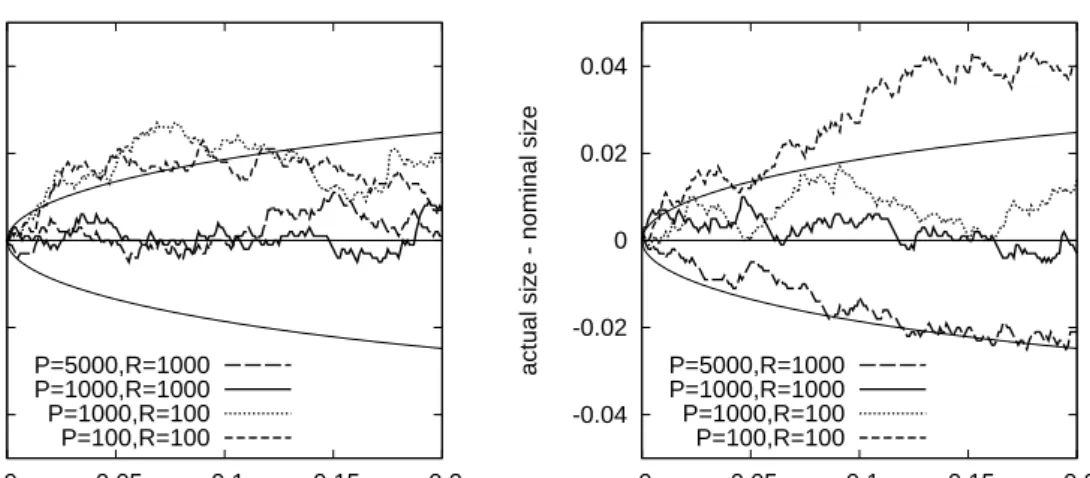
Figure 1: Size-discrepancy plots. The figure displays size-discrepancy curves, showing the dif-ference between the actual two-sided rejection rate and the nominal size (on the vertical axis) for varying nominal significance levels (on the horizontal axis). The thin lines indicate 95%
(point-wise) confidence bounds based on 1000 replications. The DGP is the SCOMDY model (3)with
standard normal marginal distributions and a bivariate product (independence) copula. The test of
equal predictive accuracy compares atcopula withρ = 0.3 against atcopula withρ = −0.3,
whereν is fixed at 5 for both copulas in the left panel andν is estimated for both copulas in the
right panel. R denotes the number of observations R in the moving in-sample window and P
denotes the number of out-of-sample evaluations.
4.1
Size
In order to assess the size properties of the test a case is required with two competing copulas that are both ‘equally (in)correct’. We achieve this in two different ways, which we call ‘non-nested null’ and ‘nested null’. Under the ‘non-nested null’ the copula in the DGP is specified as the product (or independence) copula. We then test the null hypothesis of equal predictive accuracy of two Student’s t copulas with the correlation parameter fixed at either ρ = 0.3 or ρ = −0.3. We consider two possibilities for the degrees of freedom parameter: (i) ν is also fixed for both copulas and set equal to 5, and (ii) ν is estimated at each point in time based on a moving window of lengthR. In either case the two copulas considered in the test are equally distant from the true copula. By considering these two cases we aim to investigate the effect of copula parameter estimation uncertainty on the performance of theQR,P test statistic.
size of the test is shown on Figure 1, where the null hypothesis is tested against the two-sided alternative that the averages scores of the two copulas are not equal. The left panel corresponds to case (i) where the degrees of freedom parameterν is fixed at 5, while the right panel corresponds to case (ii) with ν being estimated. In the absence of any esti-mation uncertainty in the copula parameters, we observe that the empirical rejection rate is close to the nominal significance level when both the length of the moving in-sample window and the number of out-of-sample evaluations are relatively large, that is, when R = 1000andP = 1000,5000. The test is somewhat liberal and rejects the correct null hypothesis too frequently whenR = 100andP = 100or 1000. This dependence of the size properties on the length of the moving in-sample windowRmay appear surprising at first sight, but recall that the empirical CDF transformation is used to obtain the empirical copula vectors, which still entails some estimation uncertainty. Adding parameter uncer-tainty due to the estimation of the copula parameterνresults in larger deviations from the nominal size, as shown by the right panel.
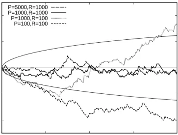
Next, we investigate the performance of the test under the ‘nested null’. The DGP in this case is taken to be a Gaussian copula with correlation coefficientρ = 0.7. We test for equal performance between the Gaussian copula and the Student’stcopula.5 For both copulas we estimate the correlation parameterρ, while the degrees of freedomν in thet copula is estimated as well. The actual/nominal size discrepancy is shown on Figure 2. Similar to the previous experiment, when the in-sample window is of reasonable length (R = 1000), the actual size of the test is within the 95%(pointwise) confidence bounds of the nominal significance level. For small estimation windows, R = 100, the test is conservative and under-rejects the null hypothesis.
4.2
Power
We evaluate the power of the test of equal predictive accuracy by performing two simula-tion experiments where one of the competing copula specificasimula-tions is correct, in the sense that it corresponds with the underlying copula DGP. Again we consider the Gaussian cop-ula and Student’stcopula, hence, we focus on the question whether theQR,P test statistic
-0.04 -0.02 0 0.02 0.04 0 0.05 0.1 0.15 0.2
actual size - nominal size
nominal size P=5000,R=1000
P=1000,R=1000 P=1000,R=100 P=100,R=100
Figure 2: Size-discrepancy plots. The figure displays size-discrepancy curves, showing the dif-ference between the actual two-sided rejection rate and the nominal size (on the vertical axis) for varying nominal significance levels (on the horizontal axis). The thin lines indicate 95%
(point-wise) confidence bounds based on 1000 replications. The DGP is the SCOMDY model (3)with
standard normal marginal distributions and a bivariate Gaussian copula withρ= 0.7. The test of
equal predictive accuracy compares atcopula with both parametersρestimated, against a
Gaus-sian copula with parameterρestimated. Rdenotes the number of observationsR in the moving
in-sample window andP denotes the number of out-of-sample evaluations. The graphs are based
on 1000 replications.
can distinguish between copulas with and without tail dependence.
We start with the DGP specified by a Student’s t copula with correlation coefficient ρ= 0.7and consider two different values of the degrees of freedom parameter,ν = 5and ν = 10. We test the tcopula specification (with both parameters estimated) against the Gaussian copula specification (with the correlation parameterρestimated). Intuitively, as thetcopula approaches the Gaussian copula asνincreases (such that the tail dependence disappears with the coefficientsλlandλuconverging to zero), the higher the value ofνin the DGP, the more difficult it is to distinguish between these two copulas.
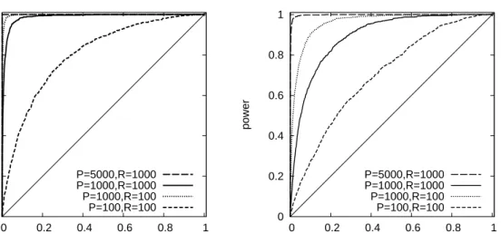
The results are shown in Figure 3 in the form of size-power curves, showing the ob-served rejection rate for different nominal significance levels. The left and right panels relate to thetcopulas withν = 5andν = 10, respectively. Here we consider a one-sided test, against the correct alternative hypothesis that the true copula has a higher average score. Note that these graphs also can be used to infer the rejection rates against the
0 0.2 0.4 0.6 0.8 1 0 0.2 0.4 0.6 0.8 1 power nominal size P=5000,R=1000 P=1000,R=1000 P=1000,R=100 P=100,R=100 0 0.2 0.4 0.6 0.8 1 0 0.2 0.4 0.6 0.8 1 power nominal size P=5000,R=1000 P=1000,R=1000 P=1000,R=100 P=100,R=100
Figure 3: Size-power curves. The figure displays size-power curves, showing the rejection rate of a one-sided test against the alternative hypothesis that the true copula has higher average score (on the vertical axis) for varying nominal significance levels (on the horizontal axis). The DGP
is the SCOMDY model (3)with standard normal marginal distributions and a bivariate Student’s
tcopula with ρ = 0.7and ν = 5 in the left panel andν = 10 in the right panel. The test of
equal predictive accuracy compares a t copula with both parameters ρ andν estimated against
a Gaussian copula with parameterρ estimated. R denotes the number of observationsR in the
moving in-sample window andP denotes the number of out-of-sample evaluations. Results are
based on 1000 replications.
rect alternative hypothesis that the other copula has a higher average score. This ‘spurious power’ at a certain nominal significance level α is equal to one minus the ‘true power’ (i.e. the rejection rate against the correct alternative) at nominal significance level1−α.
Figure 3 shows that, as expected, the test has higher power whenν = 5, that is, when the distance between the two copula specifications being compared is larger. The ‘true’ power of the test quickly goes to unity whenP = 5000. In caseR = 100andP = 100 the power is relatively low. The size-power curves are completely above the 45 degree line, showing that ‘spurious’ power of theQR,P test statistic is always below the nominal significance level.
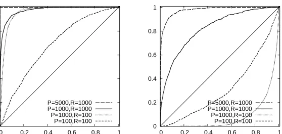
In our final experiment we consider a DGP without tail dependence by using a Gaus-sian copula with correlation coefficientρ= 0.7. We examine whether the test can distin-guish between the correct Gaussian copula and a Student’st copula with the degrees of freedom parameter fixed atν = 5orν = 10, which imposes positive tail dependence. The
0 0.2 0.4 0.6 0.8 1 0 0.2 0.4 0.6 0.8 1 P=5000,R=1000 P=1000,R=1000 P=1000,R=100 P=100,R=100 0 0.2 0.4 0.6 0.8 1 0 0.2 0.4 0.6 0.8 1 P=5000,R=1000 P=1000,R=1000 P=1000,R=100 P=100,R=100
Figure 4: Size-power curves. The figure displays size-power curves, showing the rejection rate of a one-sided test against the alternative hypothesis that the true copula has higher average score (on the vertical axis) for varying nominal significance levels (on the horizontal axis). The DGP
is the SCOMDY model (3)with standard normal marginal distributions and a bivariate Gaussian
copula withρ = 0.7. The test of equal predictive accuracy compares a tcopula with parameter
ρ estimated and ν fixed at 5 in the left panel and at 10 in the right panel, against a Gaussian
copula with parameterρ estimated. R denotes the number of observationsR in the moving
in-sample window andP denotes the number of out-of-sample evaluations. Results are based on
1000 replications.
parameterρis estimated for both the Gaussian andtcopulas. Figure 4 shows size-power curves for this experiment, withν = 5 and 10 in the left and right panels, respectively. We observe that the power of the test is higher whenν = 5, again due to the fact that the distance of thet copula from the true Gaussian copula is larger in this case. The power of the test is close to one whenP = 5000 even for very low significance levels. Also forν = 5we observe that power is still reasonable when the moving estimation window is small (R = 100) as long as the number of out-of-sample forecasts is reasonably large (P = 1000). ForP = 100power declines considerably, although we still do not observe rejection rates against the incorrect alternative exceeding the nominal significance level. This is rather different for the comparison of the Gaussian copula with at copula with ν = 10in the right panel of Figure 4. Here forR = 100we observe substantial ‘spurious’ power, in the sense that the rejection rates against the incorrect alternative are consider-able. Of course in this case the distance between the true and alternative copulas is not
large to begin with, and due to the estimation uncertainty theQR,P test statistic apparently is misguided to such an extent that it often incorrectly selects the Student’stcopula.
From the above simulation experiments we conclude that the test of equal predictive accuracy has good finite sample properties when the number of out-of-sample evaluations is sufficiently large (P = 1000, 5000).
5
Empirical application
We illustrate the use of the predictive accuracy test for comparing alternative copula spec-ifications with an empirical application. We consider daily returns on US dollar exchange rates of the Canadian dollar (CAD), Swiss franc (CHF), euro (EUR), British pound (GBP) and Japanese yen (JPY) over the period from January 1, 1980 until June 25, 2008 (7160 observations). Up to December 31, 1998, the euro series actually concerns the exchange rate of the German Deutschmark, while the euro is used as of January 1, 1999. The data are obtained from the Federal Reserve Bank of New York and concerns noon buying rates in New York. We work with two groups of three exchange rates each, that is, GBP-CHF-EUR, and CAD-JPY-EUR. The first, inter-European group presumably has a relatively high level of dependence compared to the second, inter-continental group. This is con-firmed by the unconditional correlations between the daily returns series (not shown here to save space).
We use SCOMDY models as discussed in Section 2 to model the exchange rate returns and their dependence. The conditional means and the conditional variances for the three series in each group are specified by an AR(5)-GARCH(1,1) model given by
Yj,t =cj + 5 X l=1 φj,lYj,t−l+ p hj,tεj,t hj,t =κj +γj Yj,t−1−cj − 5 X l=1 φj,lYj,t−1−l !2 +βjhj,t−1,
where κj > 0, βj ≥ 0, γj > 0 and βj +γj < 1, for j = 1, . . . ,3. The marginal distributionsFj(·)of the standardized innovationsεj,t are specified nonparametrically.
The dependence between the marginals is captured by four alternative copula specifi-cations, which we compare in terms of their relative performance in out-of-sample
den-sity forecasting. In particular, we consider the Gaussian copula, the Student’s t copula, the Clayton copula and the Gumbel copula. The Gaussian and Student’s t copula were introduced earlier in Section 4. The Clayton and Gumbel copulas are from the family of Archimedean copulas (see Nelsen (2006) for details) and are briefly described below.
Thed-dimensional Clayton copula is given by
C(u1, u2, . . . , ud;α) = d X i=1 u−i α−d+ 1 !−1/α , withα >0.
In contrast to the Gaussian and Student’stcopulas, the Clayton copula is able to capture asymmetric tail dependence. In fact, it can only exhibit lower tail dependence, while upper tail dependence is absent. In the bivariate case the lower tail dependence coefficient for the Clayton copula is λl = 2−1/α, which is increasing in the parameter α. The density function of the Clayton copula is
c(u, α) = d Y i=1 (1 + (i−1)α) ! d Y i=1 u−i (α+1) ! X u−iα−d+ 1 −1/α+d .
The Gumbel copula is specified as
C(u1, u2, . . . , ud;α) = exp − " d X i=1 (−lnui)a #1/α , withα >1.
The Gumbel copula also exhibits asymmetric tail dependence, but in contrast to the Clay-ton copula it only allows upper tail dependence, while lower tail dependence is absent. In the bivariate case the upper tail dependence coefficient for the Gumbel copula isλu = 2−21/α, which is again increasing in the parameterα. The expression for the multivari-ate Gumbel copula density is rather cumbersome and we do not show it here. Note that neither the Clayton copula nor the Gumbel copula can capture negative dependence and, thus, may not always be suitable for modeling.
We compare the one-step ahead density forecasting performance of the four copu-las using a rolling window scheme. We estimate the SCOMDY model parameters using the three-stage procedure described in Section 2. The length of the in-sample estima-tion window is set to R = 2000 observations, which leavesP = 5160 observations for out-of-sample evaluation, covering the period January 1988 - July 2008. Patton (2006)
documents a structural break in exchange rate relationships after the introduction of the euro on January 1, 1999. We therefore partition our evaluation period at this date into two sub-periods, called pre-euro and post-euro, to explore the implications of the structural break on the forecasting performance of the copula specifications. The number of obser-vations differs slightly for the pre- and post-euro periods, being equal toP = 2772and P = 2388, respectively.
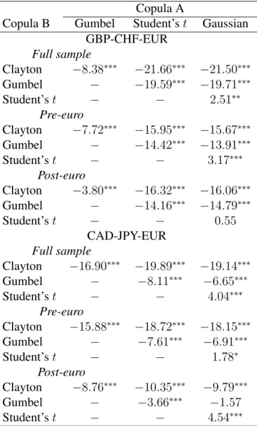
Table 1 reports the values of the pairwiseQR,P test statistic for the full sample, as well as the pre- and post-euro sub-periods, for the two groups of three exchange rates. In most cases the test makes a clear judgment about the two copulas being compared, in the sense that the null of equal predictive accuracy is generally rejected at the 1% significance level or better. The Clayton copula shows the worst performance in comparison to any other copula. The Gumbel copula is dominated by the Gaussian copula in all cases except for the CAD-JPY-EUR group during the post-euro subperiod, where the equal performance of these two copulas is not rejected at the 10% level. The Gaussian copula is, in turn, outperformed by the Student’stcopula in all cases except for the GBP-CHF-EUR group during the post-euro subperiod, where again there is not enough evidence to reject the null of equal performance of these two copulas. Thus, overall we conclude that the Student’s tcopula performs best in terms of out-of-sample multivariate density forecasts. A similar conclusion is reached by Chen and Fan (2006) based on the in-sample versions of our tests.
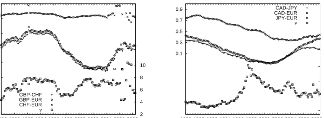
To provide more insight into these results, in Figure 5 we show the rolling window parameter estimates of the Student’s t copula for the GBP-CHF-EUR group in the left panel and for the CAD-JPY-EUR group in the right panel. The dates on the horizontal axis correspond with the end of the estimation window, that is, the moment these estimates are used for constructing the density forecast. For presentation purposes the parameter estimates are reported for every 100th day in the evaluation period. Three aspects are worth discussing in more detail. First, the estimates of the degrees of freedom parameter νexhibit substantial variation over time, ranging between6and18for the CAD-JPY-EUR group and between4and10for the GBP-CHF-EUR group. Recall that lower values ofν indicate stronger tail dependence; this is found to be the major reason for the rejection of
Table 1:Pair-wise tests for out-of-sample performance of copulas
Copula A
Copula B Gumbel Student’st Gaussian GBP-CHF-EUR Full sample Clayton −8.38∗∗∗ −21.66∗∗∗ −21.50∗∗∗ Gumbel − −19.59∗∗∗ −19.71∗∗∗ Student’st − − 2.51∗∗ Pre-euro Clayton −7.72∗∗∗ −15.95∗∗∗ −15.67∗∗∗ Gumbel − −14.42∗∗∗ −13.91∗∗∗ Student’st − − 3.17∗∗∗ Post-euro Clayton −3.80∗∗∗ −16.32∗∗∗ −16.06∗∗∗ Gumbel − −14.16∗∗∗ −14.79∗∗∗ Student’st − − 0.55 CAD-JPY-EUR Full sample Clayton −16.90∗∗∗ −19.89∗∗∗ −19.14∗∗∗ Gumbel − −8.11∗∗∗ −6.65∗∗∗ Student’st − − 4.04∗∗∗ Pre-euro Clayton −15.88∗∗∗ −18.72∗∗∗ −18.15∗∗∗ Gumbel − −7.61∗∗∗ −6.91∗∗∗ Student’st − − 1.78∗ Post-euro Clayton −8.76∗∗∗ −10.35∗∗∗ −9.79∗∗∗ Gumbel − −3.66∗∗∗ −1.57 Student’st − − 4.54∗∗∗
Note: The table present values of theQR,P test statistic of
the null hypothesis of equal predictive accuracy of two al-ternative copula specifications. Positive (Negative) values indicate better performance of copula A (B). The asterisks
∗,∗∗and∗∗∗indicate significance at (two-sided)10%,5%
and1%levels respectively. The length of the moving in-sample estimation window is equal to R = 2000 in all cases. The number of observations in the out-of-sample period is equal toP= 5160for the full sample,P = 2772
for the pre-euro period and P = 2388 for the post-euro period.
0.5 0.6 0.7 0.8 0.9 1 1988 1990 1992 1994 1996 1998 2000 2002 2004 2006 2008 2 4 6 8 10 GBP-CHF GBP-EUR CHF-EUR ν 0.1 0.3 0.5 0.7 0.9 1988 1990 1992 1994 1996 1998 2000 2002 2004 2006 2008 6 10 14 18 CAD-JPY CAD-EUR JPY-EUR ν
Figure 5:Parameter estimates of the Student’stcopula over time for the two groups of exchange rates: GBP-CHF-EUR in the left panel and CAD-JPY-EUR in the right panel. The parameter
esti-mates are reported for every100th day in the evaluation period. Year labels indicate the beginning
of the corresponding year.
the Gaussian copula against thetcopula.
Second, the correlation estimates clearly differ among the exchange rate pairs within each group. This suggests that the one-parameter Clayton and Gumbel copulas are not suitable as they are not able to reflect these differences. This explains the inferior fore-casting performance of these two copulas relative to the Gaussian andtspecifications.
Third, we observe slowly changing correlations over time. There is some evidence for a structural break due to the euro introduction on January 1, 1999. The post-euro period is characterized by slowly increasing increasing correlations for CAD-EUR, CAD-JPY and JPY-EUR, while they were slowly decreasing before. The same is true for the exchange rate pairs in the other group, that is the GBP-CHF and GBP-EUR correlations also start increasing after the introduction of the euro. The CHF-EUR correlations are close to unity over the whole sample period, with a slight tendency to increase during the post-euro period. This creates some challenges for the maximization procedure and results in somewhat unstable estimates around 2006-2008. It is also more difficult to distinguish the Gaussian copula from the Student’stcopula when the correlation is close to one. In the limiting case of unit correlation the Gaussian copula also has tail dependence.6 All these
factors contribute to the inability of the test to reject the equal performance between the 6The correlations estimates obtained for the Gaussian copula specifications are very similar to the values
Gaussian copula and the Student’stduring this subperiod.
6
Summary and discussion
In this paper we have introduced a new statistical test for comparing alternative parametric copula specifications in the context of multivariate density forecasts. The test is based on the Kullback-Leibler Information Criterion (KLIC), which is a measure of distance of the candidate copula specifications to the true copula. Although the true copula is unknown, score differences can be used to compare copula specifications pair-wise; the copula with the smallest average KLIC is considered to be superior. The main difference with other tests for competing copula families is that we use an out-of-sample measure for the suitability of the copulas.
Following Giacomini and White (2006), the potential problem that parameter estima-tion uncertainty might affect the distribuestima-tion of test statistics is avoided by considering this aspect as an integral part of the forecasting method. The resulting test is valid un-der general conditions, allowing for parameter estimation uncertainty and for comparing either nested or non-nested copula families.
In practice, the test would be used to compare two competing copula families by test-ing for equal average scores against the two-sided alternative that one of the families receives a higher average score. However, to distinguish between true power and spurious power (rejections of the null hypothesis in favor of the wrong copula family) we presented Monte Carlo simulation results in the form of one-sided size-power plots. The Monte Carlo results suggest that the proposed test has satisfactory size and power properties in finite samples. Spurious power is observed, but only in cases of very small estimation windows and alternative copula specifications that are not very different from each other in terms of their dependence properties.
In an application to daily exchange rate returns of several major currencies against the US dollar we found that the Student’stcopula is clearly favored over Gaussian, Gumbel and Clayton specifications. This suggests that these exchange rate returns are character-ized by symmetric tail dependence.
References
Amisano, G. and Giacomini, R. (2007). Comparing density forecasts via weighted likeli-hood ratio tests. Journal of Business and Economic Statistics,25,177–190.
Bao, Y., Lee, T.-H. and Salto˘glu, B. (2007). Comparing density forecast models. Journal of Forecasting,26,203–225.
Berg, D. (2007). Copula goodness-of-fit testing: An overview and power comparison. Working paper, Norwegian Computing Center.
Berg, D. and Bakken, H. (2007). A copula goodness-of-fit approach based on the condi-tional probability integral transform. Working paper, Norwegian Computing Center. Breymann, W., Dias, A. and Embrechts, P. (2003). Dependence structures for multivariate
high-frequency data in finance. Quantitative Finance,3,number 1, 1–14.
Chen, X. and Fan, Y. (2005). Pseudo-likelihood ratio tests for semiparametric multivariate copula model selection. Canadian Journal of Statistics,33,389–414.
Chen, X. and Fan, Y. (2006). Estimation and model selection of semiparametric copula-based multivariate dynamic models under copula misspecification. Journal of Econo-metrics,135,125–154.
Cherubini, U., Luciano, E. and Vecchiato, E. (2004). Copula Methods in Finance. Wiley Finance Series. Wiley, Chicester.
DeHeuvels, P. (1979). La fonction de d´ependance empirique et ses propri´et´es. Un test non param´etrique d’ind´ependance.Acad´emie Royale de Belgique. Bulletin de la Classe de Sciences,5`eme Serie 65,274–292.
Fermanian, J.-D. (2005). Goodness-of-fit tests for copulas. Journal of Multivariate Analysis,95,119–152.
Genest, C., Quessy, J.-F. and R´emillard, B. (2006). Goodness-of-fit procedures for cop-ula models based on the probability integral transformation. Scandinavian Journal of Statistics,33,337–366.
Genest, C. and R´emillard, B. (in press). Validity of the parametric bootstrap for goodness-of-fit testing in semiparametric models. Annales de l´Institut Henri Poincar´e - Proba-bilit´es et Statistiques.
Genest, C., R´emillard, B. and Beaudoin, D. (in press). Omnibus goodness-of-fit tests for copulas: A review and a power study. Insurance: Mathematics and Economics.
Giacomini, R. and White, H. (2006). Tests of conditional predictive ability.Econometrica,
74,1545–1578.
Joe, H. (1997). Multivariate Models and Dependence Concepts. London: Chapman & Hall.
Kole, E., Koedijk, K. and Verbeek, M. (2007). Selecting copulas for risk management.
Journal of Banking and Finance,31,2405–2423.
Malevergne, Y. and Sornette, D. (2003). Testing the Gaussian copula hypothesis for financial assets dependence. Quantitative Finance,3,231–250.
Mitchell, J. and Hall, S.G. (2005). Evaluating, comparing and combining density forecasts using the KLIC with an application to the Bank of England and NIESR ‘fan’ charts of inflation. Oxford Bulletin of Economics and Statistics,67,995–1033.
Nelsen, R.B. (2006). An Introduction to Copulas, Second edn. New York: Springer Verlag.
Panchenko, V. (2005). Goodness-of-fit tests for copulas. PhysicaA,355,176–182. Patton, A.J. (2006). Modelling asymmetric exchange rate dependence. International
Economic Review,47,527–556.
Patton, A.J. (2008). Copula-based models for financial time series. In Handbook of Financial Time Series (eds T.G. Andersen, R.A. Davis, J.-P. Kreiss and T. Mikosch). Berlin: Springer-Verlag.
Rivers, D. and Vuong, Q. (2002). Model selection tests for non-linear dynamic models.
Rosenblatt, M. (1952). Remarks on a multivariate transformation.Annals of Mathematical Statistics,23,470–472.
Sklar, A. (1959). Fonction de r´epartitions `andimensions et leurs marges. Publications de l’Institut Statistique de l’Universit´e de Paris,8,229–231.
Vuong, Q. (1989). Likelihood ratio tests for model selection and non-nested hypotheses.