HAL Id: hal-02090886
https://hal.archives-ouvertes.fr/hal-02090886v2
Preprint submitted on 17 Apr 2019
HAL
is a multi-disciplinary open access
archive for the deposit and dissemination of
sci-entific research documents, whether they are
pub-lished or not. The documents may come from
teaching and research institutions in France or
abroad, or from public or private research centers.
L’archive ouverte pluridisciplinaire
HAL
, est
destinée au dépôt et à la diffusion de documents
scientifiques de niveau recherche, publiés ou non,
émanant des établissements d’enseignement et de
recherche français ou étrangers, des laboratoires
publics ou privés.
Longitudinal autoencoder for multi-modal disease
progression modelling
Raphäel Couronné, Maxime Louis, Stanley Durrleman
To cite this version:
Raphäel Couronné, Maxime Louis, Stanley Durrleman. Longitudinal autoencoder for multi-modal
disease progression modelling. 2019. �hal-02090886v2�
disease progression modelling
Raphael Couronne1,2, Maxime Louis1,2, and Stanley Durrleman1,2
1
Sorbonne Universites, UPMC Univ Paris 06, Inserm, CNRS, Institut du cerveau et de la moelle (ICM)
2 Inria Paris, Aramis project-team, 75013, Paris, France
Abstract. Imaging modalities and clinical measurement, as well as their time progression can be seen as heterogeneous observations of the same underlying disease process. The analysis of sequences of multi-modal observations, where not all modalities are present at each visit, is a chal-lenging task. In this paper, we propose a multi-modal autoencoder for longitudinal data. The sequences of observations for each modality are encoded using a recurrent network into a latent variable. The variables for the different modalities are then fused into a common variable which describes a linear trajectory in a low-dimensional latent space. This la-tent space is mapped into the multi-modal observation space using sep-arate decoders for each modality. We first illustrate the stability of the proposed model through simple scalar experiments. Then, we illustrate how information can be conveyed from one modality to refine predictions about the future using the learned autoencoder. Finally, we apply this approach to the prediction of future MRI for Alzheimer’s patients.
Keywords: Longitudinal·Multi-modal·Autoencoder
1
Introduction
The longitudinal pattern of progression of a disease contains more information than a static observation. Leveraging this information is a key problem in ma-chine learning for healthcare, complicated by to the nature of clinical datasets. These datasets may contain very heterogeneous observations from various modal-ities of subjects at multiple time points, such as clinical scores, imaging and biological samples. They include missing values, often by design: not all modal-ities are observed at each visit. Besides, the number of observations and their time spacing vary between subjects. For these reasons, the analysis of multiple modalities and their time dynamic at once is a challenging task.
Linear mixed effect model estimated via EM and their extension to the non-linear case [4, 5] were developed for the analysis of unimodal longitudinal data. More recently, recurrent auto-encoder [9, 11] offer a way to encode trajectories into a low-dimensional embedding, allowing to perform unsupervised clustering of the trajectories [2]. Riemannian geometry based approaches such as [6,10] offer ways to learn sub-manifolds of the observation space with a system of coordinate adapted to the progression of the modality observed in the data.
2 Raphael Couronne , Maxime Louis, and Stanley Durrleman
On the other hand, various unsupervised methods exist to fuse information from multiple modalities but from a single time snapshot. In [1, 8], the authors propose to learn a common embedding for multiple modalities auto-encoding, merging the information from all modalities and allowing the generation of miss-ing modalities. In [7], unsupervised features are learned from heterogeneous health data as a dimensionality reduction method before machine learning tasks. In [12], combining time and multi-modal approaches, the authors propose a setting for multi-modal time-series embedding. But their design does not handle missing modalities, common in clinical data sets. Besides, the fusion of the in-formation from the different modalities is done at each time step and not on the progression pattern globally, thus decreasing the importance of the dynamics of each modality in the encoding.
To address these limitations, we propose a new setting for longitudinal multi-modal encoding. We extend to the multi-multi-modal case the approach of [6]. Each modality is first separately encoded using a recurrent neural network. A fu-sion network is then used to merge the obtained representations into a unique representation, which describes the multi-modal trajectory of the subject as a
time-parametrized linear trajectory in a latent space Z. Then, this trajectory
is decoded using a different neural network for each modality, which generates continuously varying trajectories of data changes. This setting allows to handle multiple modalities even when not all of them are observed at each visit and it can handle any number of visits and any time spacing between the visits. Finally, extrapolation in the latent space allows for prediction of the future of each modality and we show on a synthetic dataset and on the ADNI database using cognitive scores and MRI jointly that the predictive power is enhanced by the fusion of each modality embeddings.
In section 2 we explain the proposed model, in section 3 we present exper-imental results highlighting the stability of the method on synthetic and real data sets and we show how the information from one modality that contributes to the encoding allows to refine prediction of the future of another modality.
2
Methods
We set a longitudinal dataset which contains repeated observations of subjects, where the observations at each time point contain a various combination of
modalities amongM ∈Nmodalities. For any subjecti∈ {1, . . . , N}whereN ∈
N and for any modalitym∈ {1, . . . , M}, we have a sequence (ym
ij, tmij)j=1,...,nm i
of observationsym
ij of observed at timestmij.
2.1 Decoding : Non linear mixed effect model
We setd∈Nand consider ad-dimensional latent spaceZ =Rdand its canonical
basis (ei)i=1,...,d. Then, in the spirit of random slopes and intercepts models, we
consider trajectories in Z of the form l(t) = eη(t−τ)e1+Pd
i=2λ
ie
i where
Z z RNN 2 Z RNN 1 RNN 2 Z Modality 1 LONGITUDINAL OBSERVATIONS Reconstructed trajectory LATENT SPACE
TRAJECTORY MODEL PARAMETRIZED TRAJECTORIESRECONSTRUCTED
TIME-Average trajectory Subject’s trajectory Reconstructed trajectory Modality 2 Z1 Fusion
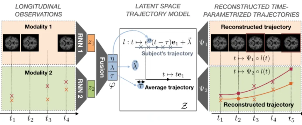
Fig. 1: Description of the proposed longitudinal autoencoder.
direction and are translated in any direction orthogonal to e1, so that the λs
play the role of random intercepts. η controls the pace of progression while τ
allows for a time shift between the trajectories. We consider that thei-th subject
follows a trajectory of this form with parametersϕi= ηi, τi, λ2i, . . . , λdi
.
For each considered modalitym, we consider a nonlinear mappingΨwmwhich
maps Z on a subspace of the m-th modality observation space. This
trans-ports the mixed-effect model formulated inZinto the corresponding observation
spaces. Note that the apparent rigidity of the family of trajectories considered in
Z is not restrictive provided the mappingsΨwm are flexible enough. In practice,
theΨwmare neural networks, de-convolutional for images and fully connected for
scalars. The right half of Figure 1 illustrates the procedure. Overall, this setting can be viewed as a non-linear mixed-effect model where the random effects are
theϕi’s and the fixed effects are the parameters of the mappingsΨwm.
2.2 Encoding
Individual parametersϕiare estimated via the use of an encoder network. More
precisely, each modality is first processed by a dedicated Recurrent Neural Net-work (RNN), to get modality-wise representations. To correct for the varying spacings between the observations, we provide to the RNN the visit times, pre-viously normalized to zero-mean and unit variance.
We then concatenate the obtained representations, and use a fully-connected network to merge the representations. The given architecture alllows fast infer-ence for new subjects, and is trainable end to end. Besides, the fusion operation is learned so as to produce a single vector which contains the most information about the reconstruction of the whole sequences of all the modalities. The left part of Figure 1 illustrates the procedure.
4 Raphael Couronne , Maxime Louis, and Stanley Durrleman
2.3 Regularization, cost function and optimization
To enforce some structure in the latent space and in the family of
trajecto-ries obtained, we set the following regularization on the individual variable Φi:
r(η, τ,(λi)i=2,...,d) =η2+τ2+Pdj=2(λj)2. This regularization models theη
vari-able to be distributed along a zero-centered normal distribution, which allows the pace of progression to vary typically between 0.2 and 5. times the mean
velocity. The τ variable is regularized the same way. This regularization is not
arbitrary: during each run, the observation times tm
ij are rescaled to zero-mean
unit variance, and thusτ can handle delays between subjects of order the
stan-dard deviation of the observation ages.
Overall, the optimized cost function for one subject is the regularization cost
added to the`2 reconstruction cost summed over all modalities:
C((wm)m, η, τ,(λi)i) =r(η, τ,(λi)i) + X m 1 σ2 m nm i X j=1 kymij −Ψwm(li(t m ij))k 2 2 (1)
where the (σm)mare trade-off parameters between each modality and the
reg-ularization. We set an automatic update rule for these parameters after each batch by setting them to the empirical quadratic errors in reconstruction for the modality over the batch. The estimation is achieved by stochastic gradient descent with the Adam optimizer [3] and a batch size of 32 subjects. The De-coders are either fully connected or de-convolution networks depending on the kind of modality considered, with standard architectures. The encoders are ei-ther Elman networks or Elman networks working on features extracted using a convolution network in the case of images. All networks are trained end to end using back-propagation and the PyTorch library. A complete code to reproduce these experiments will be released upon publication of the paper.
3
Experimental results
3.1 Cognitive scores: proof of concept
As in [10], we apply our model on repeated measurement of 4 normalized cogni-tive score extracted from the ADNI cohort, respeccogni-tively associated with memory, language, praxis and concentration. We include the 248 MCI-converter subjects, followed for an average of 3 years, over 6 visits. We conduct 2 experiments in order to assess the robustness of the method, and report estimated average trajectories in Figure 2, as well as individual reconstruction errors in Table.1, computed from a patient-wise 10-fold cross validation.
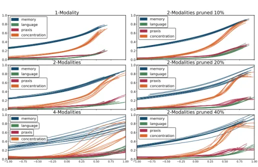
First, we apply our model on an increasing partitioning of input feature. We consider 3 cases: selecting all scores at once as one modality, selecting separately memory+language and praxis+concentration as two modalities, and selecting each one separately. We note the overall good stability of the average model over multiple multi-modal architectures, with stability decreasing in the 4-modalities scenario, arguing for a concatenation of the consistent features.
0.0 0.2 0.4 0.6 0.8 1.0 1-Modality memory language praxis concentration 0.0 0.2 0.4 0.6 0.8 1.0 memory 2-Modalities language praxis concentration 1.00 0.75 0.50 0.25 0.00 0.25 0.50 0.75 1.00 0.0 0.2 0.4 0.6 0.8 1.0 4-Modalities memory language praxis concentration 0.0 0.2 0.4 0.6 0.8 1.0 2-Modalities pruned 10% memory language praxis concentration 0.0 0.2 0.4 0.6 0.8
1.0 memory2-Modalities pruned 20%
language praxis concentration 1.00 0.75 0.50 0.25 0.00 0.25 0.50 0.75 1.00 0.0 0.2 0.4 0.6 0.8 1.0 2-Modalities pruned 40% memory language praxis concentration
Fig. 2: Left: average trajectories for the 10 folds, with increasing partitioning of the input features. Right: average trajectories for the 10 folds, with increasing pruning of the praxis+concentration modality.
In our second experiment, we assess the robustness of the model with the number of visits per subjects. To this end we consider the 2-modalities scenario, and perform a pruning of the dataset, removing an increasing number of vis-its of the second modality, i.e. praxis+concentration per subjects. Datasets are obtained from pruning frequencies of respectively 10%, 20% and 40%. Here we also observe an overall good stability of the average trajectory over pruning frequency.
3.2 A synthetic dataset
To test the proposed setup in realistic conditions, we generate a synthetic multi-modal data set comprising 300 subjects observed 7 times on average. The first modality is a 2D image of a cross, with varying arm lengths and angles while the second modality consists of two scores with a sigmoid-like growth. We set a
time reparametrization functions with parameters a1, a2 defined by: sa,b(t) =
Partitioning Pruning
1-mod 2-mod 4-mod 2-mod 10% 2-mod 20% 2-mod 40% Train (x10−3) 6.7 3.8 / 9.7 21.1 / 2.2 / 5.6 / 5.3 4.9 / 11.3 4.1 / 11.5 4.5 / 14.6
Test (x10−3) 7.8 5.1 / 10.6 24.7 / 3.3 / 7.1 / 5.2 4.9 / 11.7 5.0 / 11.9 5.4 / 15.5 Table 1: Mean 10-fold reconstruction error for the 2 cognitive scores experiments for each modality respectively
6 Raphael Couronne , Maxime Louis, and Stanley Durrleman
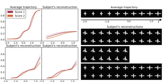
Fig. 3: Left: average trajectory and reconstruction examples for the scalar data. Right: average trajectory and some reconstructions for the image data.
t+asign(t)t2+bt3. To generate an individual, we sample two sets of parameters
(ak, bk)k=1,2. These serve to reparametrize a scenario of score increase: the k
-th score for -the subject at timet is given by σ◦sak,bk where σ is the sigmoid
function. Then, the arms lengthsL1, L2 for the images of the subject at timet
are given by L1 =σ◦s(a2−a1)+εa1,(b2−b1)+εb1, L2 =σ◦s(a2+a1)+εa2,(b2+b1)+εb2
where the ε are samples from a zero-mean normal distribution and constant
with time. Finally, the arm angles are sampled along a normal distribution but are not informative of the synthetic disease process. This design is so that the images contain, in an intricate way, information about the progression of the
scores materialized through the a1, a2, b1, b2 variables. The two modalities are
different noisy facets of a common underlying process.
We perform a patient-wise 10-fold estimation of the model this data set. Figure 3 shows the obtained average trajectory for the first fold, as well as the reconstructions of some subjects images and scores observations. We evaluate and average for all folds the test and train reconstruction errors. For the cross, the test error is 2.0 10−8±8.10−9while the train error is 1.7 10−8±3.9 10−9. For the
scores, the test error is 7.10−3±3.10−3while the train error is 7.10−3±3.10−3.
This shows that the model generalizes well to unseen data.
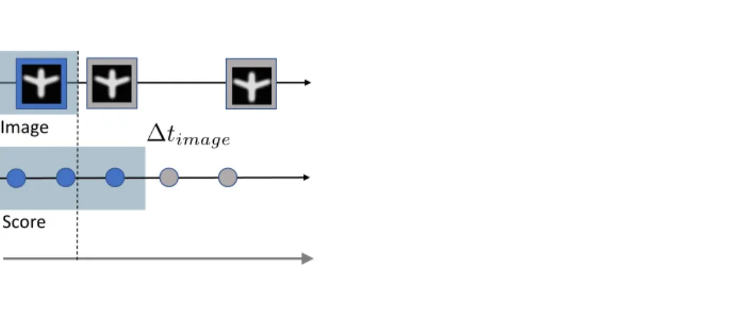
We use the trained model to predict the future scores on the test data. We do so by decoding the extrapolation of the latent trajectory encoded by the model. We repeat this experiment by gradually removing the last observations of the image modality, to look at the impact of this modality on the predictive power of the model. Figure 4 shows the experimental setup and the results. As the time span of the observed images shrinks, the prediction deteriorates: when more image data is available, the score prediction is more accurate. This shows the ability of the model to find a relevant common representation for the progressions of the different modalities.
3.3 Application to Alzheimer’s disease future image prediction
On the 248 patients of section 3.1, we apply the same model on the 217 that have at least 1 MRI observation, leading to a total of 1199 cognitive scores mea-surements and 1441 MRIs. We work on both the MRI images and the cognitive
scores. The MRI images are rigidly aligned and sub-sampled to 643 resolution.
Note that the subjects do not have both the MRI and the cognitive scores mea-surements at each visit.
Figure 5 shows one of the estimated average trajectory for the MRI modality. We evaluate and average for all folds the test and train reconstruction errors on
both modalities. For the MRI, the test error is 2.5 10−3±6.10−5while the train
error is 2.4 10−3±2. 10−5. For the scores, the test error is 2.2 10−2±3. 10−3
while the train error is 1.7 10−3±6.10−4. This shows that the model generalizes
well to unseen data.
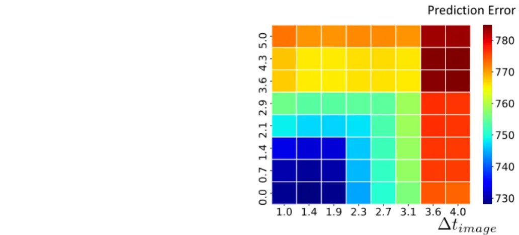
We then perform the same prediction task as in the previous section: we attempt to predict the future MRI from past data, using a variable amount of score data in the past. Figure 5 shows the prediction errors for different time horizon. Once again, the errors increase as we feed the model with less cognitive scores measurements. This shows that the model captures information contained in the cognitive scores progression to refine the MRI prediction.
4
Conclusion and perspectives
We extended on a deep autoencoder architecture with a mixed effect latent space to propose a practical framework for modeling multi-modal longitudinal data, trainable end-to-end. This allows for analysis of heterogeneous longitudi-nal datasets, deriving a model-wise average trajectory, as well as condensed pa-tient representations. We study its robustness toward modalities partitioning and
Image Score 0 1 2 3 Unseen Seen Test
Duration to last score observation
Prediction Error
8 Raphael Couronne , Maxime Louis, and Stanley Durrleman
Prediction Error Average Trajectory
Fig. 5: Left: average trajectory. Right: prediction error, in the same setup as in Section 3.2
dataset pruning and illustrate its utility in both synthetic and real scenarios. In the future we plan to model the progression of more modalities at once. This work has been partially funded by the European Re-457search Council (ERC) un-der grant agreement No 678304, European Unions Horizon4582020 research and innovation programme under grant agreement No 666992, and the459program Investissements davenir ANR-10-IAIHU-06.
References
1. Chartsias, A., Joyce, T., et al.: Multimodal mr synthesis via modality-invariant latent representation. IEEE transactions on medical imaging (2018)
2. Falissard, L., Fagherazzi, G., Howard, N., Falissard, B.: Deep clustering of longi-tudinal data. arXiv preprint arXiv:1802.03212 (2018)
3. Kingma, D.P., Ba, J.: Adam: A method for stochastic optimization. arXiv preprint arXiv:1412.6980 (2014)
4. Laird, N.M., Ware, J.H.: Random-Effects Models for Longitudinal Data. Biometrics (dec 1982)
5. Lindstrom, M.J., Bates, D.M.: Nonlinear Mixed Effects Models for Repeated Mea-sures Data. Biometrics46(3), 673 (sep 1990)
6. Louis, M., et al.: Riemannian geometry learning for disease progression modelling. In: International Conference on Information Processing in Medical Imaging (2019) 7. Miotto, R., Li, L., Kidd, B.A., Dudley, J.T.: Deep patient: An unsupervised rep-resentation to predict the future of patients from the electronic health records. Scientific Reports6, 26094 EP – (05 2016),https://doi.org/10.1038/srep26094
8. Ngiam, J., Khosla, A., Kim, M., et al.: Multimodal deep learning. In: Proceedings of the 28th international conference on machine learning (ICML-11) (2011) 9. Rumelhart, D.E., Hinton, G.E., Williams, R.J., et al.: Learning representations by
back-propagating errors. Cognitive modeling5(3), 1 (1988)
10. Schiratti, J.B., et al.: Learning spatiotemporal trajectories from manifold-valued longitudinal data. In: Advances in Neural Information Processing Systems (2015)
11. Srivastava, N., Mansimov, E., et al.: Unsupervised learning of video representations using lstms. In: International conference on machine learning (2015)
12. Yang, X., et al.: Deep multimodal representation learning from temporal data. In: IEEE Conference on Computer Vision and Pattern Recognition (2017)