Dictionary Learning Based Feature Level
Domain Adaptation for Cross-scene
Hyperspectral Image Classification
Minchao Ye, Yuntao Qian,
Member, IEEE
, Jun Zhou,
Senior Member, IEEE
and
Yuan Yan Tang,
Fellow, IEEE
Abstract
A big challenge in hyperspectral image (HSI) classification is small size of labeled data for classifier learning. In real remote sensing applications, we always face the situation that an HSI scene is not labeled at all or is with very limited number of labeled pixels, but we have sufficient labeled pixels in another HSI scene with similar land cover classes. In this paper, we undertake classification on a target HSI scene containing no labeled sample or only few labeled samples with the help of a similar source HSI scene having relatively large size of labeled samples. We name this classification problem as cross-scene classification. The main challenge of cross-scene classification is spectral shift, i.e., even for the same class in different scenes, their spectral distributions may have significant deviation. As all or most training samples are drawn form the source scene and the prediction is performed on the target scene, the difference in spectral distribution would greatly deteriorate the classification performance. To solve this problem, we propose a dictionary learning based feature level domain adaptation technique, which aligns the spectral distributions between source and target scenes by projecting their spectral features into a shared low-dimensional embedding space by multitask dictionary learning. The basis atoms in the learned dictionary represent the common spectral components, which span a cross-scene feature space to minimize the effect of spectral shift. After the HSIs of two scenes are transformed into the shared space, any traditional HSI classification approaches can be used. In this paper, sparse logistic regression is selected as the classifier. To be more specific, if there are a few labeled pixels in the target domain, multitask sparse logistic regression is used to further promote the classification performance. The experimental results on both synthetic and real HSIs show the advantages of the proposed method for cross-scene classification.
Index Terms
Hyperspectral image, cross-scene classification, domain adaptation, dictionary learning, multitask learning.
M. Ye and Y. Qian are with the Institute of Artificial Intelligence, College of Computer Science, Zhejiang University, Hangzhou 310027, China (e-mail:[email protected]).
J. Zhou is with School of Information and Communication Technology, Griffith University, Nathan, Queensland 4111, Australia. Y. Y. Tang is with the Faculty of Science and Technology, University of Macau, Macau 999078, China.
I. INTRODUCTION
Pixel classification is an important application on hyperspectral images (HSI). A challenge in HSI classification is small size of training data, which makes the training models ill-posed. In order to solve this problem, semi-supervised learning and active learning are widely used in HSI classification. Semi-supervised learning makes use of both labeled and unlabeled data to train a classifier, including semisupervised SVM [1], [2], graph-based semisupervised learning [3], manifold-based semisupervised learning [4]. Active learning is an interactive information extraction approach [5]–[7]. During training procedure, it selects informative unlabeled samples and label them, which minimizes the cost of labeling to reach a good classification performance. Both semisupervised learning and active learning approaches assume that the pixels belonging to the same land cover class follow an identical distribution in the feature space.
In real remote sensing applications, we always encounter the situation that an HSI scene (called target scene) to be classified has only very few labeled samples or even not any labeled sample due to high labor costs of labeling or other limitations. On the contrary, other similar scenes (source scenes) may have sufficient labeled samples. In this case, a natural idea is to make use of the class-specific information in source scenes to help target scene classification. we call this problem as cross-scene classification. For example, if a city in somewhere suffered from a natural disaster such as earthquake, flooding, or hurricane, we want to understand the field condition and assess the disaster losses through hyperspectral remote sensing and HSI processing techniques including classification. It is not realistic to obtain many labeled samples in the captured HSIs on this site, but we can easily found some HSIs with more labeled samples captured from similar cities. These cities share a common set of land cover objects. For example, in urban areas there always are roads, buildings, rivers, trees, grasses, et al, while in rural areas there commonly have fields with various crops. The common land cover classes make it possible to transfer knowledge between similar HSI scenes.
The most straightforward method for cross-scene classification is to use the source domain samples directly. When no labeled samples are available in the target scene, the source domain samples can be directly employed to train a classifier. When a few labeled samples are available in the target scene, we can merge the labeled samples in both scenes for training. However this simple way suffers from spectral shift, i.e., pixels belonging to same land cover class may vary in spectral distribution from two different HSI scenes. This phenomenon is also called covariate shift, population drift or dataset shift [4], [8]–[12], which occurs when the training and testing scenes are spatially or temporally different. The spectral shift is caused by many factors, including different atmospheric and light conditions at the image acquisition stage, different sensor nonlinearities, different substance compositions of the same land cover class in different sizes and times, etc. [13]. Therefore, even though a large number of training data are available in the source scenes, the classifiers trained from those data or the combined data from both source and target scenes may perform poorly on the testing samples from the target scene [14], [15]. Therefore, a more complex strategy is necessary to better solve the cross-scene classification problem.
The key issue of cross-scene classification is to reduce the spectral shift in feature level or classifier level by domain adaptation. Classifier level domain adaptation tunes the parameters and structures of a classifier model
during training procedure to make the classifier generalize to target domain. Bruzzone and Prieto [13] proposed a maximum-likelihood (ML) based retraining method to tackle spectral shift in multi-temporal remote sensing images. Firstly, an ML classifier is trained on source scene in a supervised manner, producing the a priori probability and conditional density for each class. Then the statistical distribution of pixels in target scene is represented by a mixed density distribution with as many components as the classes to be recognized. Finally, retraining this ML classifier in target domain becomes a mixture density estimation problem that can be solved by expectation maximization (EM) algorithm. Alternatively, Rajan et al [8] used binary hierarchical classifier (BHC) to solve this problem. The BHC involves recursively decomposing a multiclass (C-classes) problem into (C−1) binary metaclass problems by building a binary tree. BHC takes similarity among classes into consideration, where similar classes are in the same metaclass (parent node). The structure of BHC tree conveys the relationship between classes, which can be shared between source and target scenes. The BHC transfers the hierarchy of the classes from source scene to target scene and retrains each binary classifier via EM algorithm. Sun et al [11], [12] applied support vector machine (SVM) with cross-domain kernels for domain adaptation, whose cost function combines two factors simultaneously, one is minimizing the distribution distance between two domains in reproducing kernel Hilbert space, and the other is minimizing the structural risk function of SVM. The classifier level domain adaptation is focused on modifying the classifier while the transformation between source and target domains is not explicitly displayed, therefore, dependence on specific classifier is its main disadvantage.
Feature level domain adaptation attempts to directly adjust the feature space domains of source and target data sets to decrease their discrepancy of distribution, after that any classifier can be used. Tuia et al [16] proposed manifold alignment with graph matching, which assumes that source and target data lie on two different manifolds. Graph matching is used for finding a mapping to align these two manifolds, by which target data can be transformed into the source domain, or vice versa. Thus the classifier trained from source scene can be applied on the target scene. However, finding a precise graph matching is a difficult task, especially with a large difference between source and target scenes in terms of class distribution and spectral distribution.
In this paper, we propose a dictionary learning based feature-level domain adaptation method which projects the spectral feature spaces of source and target scenes into a shared subspace spanned by atoms in the dictionary. In this shared subspace, the spectral shift between two domains is reduced. A multitask joint dictionary learning (MTJDL) scheme is used to extract the common components between target and source scenes. Dictionary learning is to find the intrinsic subspace that can sparsely represent the data in the form of a linear combination of basis atoms. Multitask learning is a powerful learning technique which binds several related learning tasks to improve their performance by a shared model [17]. MTJDL combines the advantages of both dictionary learning and multitask learning, which provides cross-scene feature extraction, domain adaptation, and dimensional reduction at the same time, all of which are critical factors to improve the performance of cross-scene HSI classification. The coding coefficient over the learned dictionary is utilized as cross-scene feature, by which any classifier can be adopted.
The rest of this paper is organized as follows. Section II introduces the basic theory of domain adaptation, especially feature level domain adaptation, and its relation with cross-scene HSI classification. Section III presents MTJDL based domain adaptation for cross-scene feature extraction and the subsequent classification algorithms for
Fig. 1. Band 120 of Indiana image in which two scenes are marked.
Band
50 100 150 200Reflectance
0 1000 2000 3000 4000 5000 6000 7000 Source: Soybeans-CleanTill-EW Source: Corn-CleanTill-EW Target: Soybeans-CleanTill-EW Target: Corn-CleanTill-EW (a)Band
50 100 150 200Reflectance
1000 2000 3000 4000 5000 6000 Source: Soybeans-CleanTill-EW Source: Corn-CleanTill-EW Target: Soybeans-CleanTill-EW Target: Corn-CleanTill-EW (b)Fig. 2. Spectral signatures of two land cover classes Soybeans-CleanTill-EW and Corn-CleanTill-EW in two scenes of Indiana image. (a) Spectral signatures of randomly selected pixels. (b) Mean spectral signatures.
cross-scene HSI classification. Experiments on both synthetic and read-world data sets are reported in Section IV to show the benefit brought by domain adaptation. At the end, conclusions are drawn in Section V.
II. CROSS-SCENEHSICLASSIFICATION AND DOMAIN ADAPTATION
Due to spectral shift, classical statistical learning algorithms are no longer valid for cross-scene HSI classification as they are always based on the assumption that both training and testing samples are drawn from an identical distribution. To show the shift of spectral distribution between two scenes, we select two spatially distant regions of interest from AVIRIS Indiana HSI image which covers a large area (see Fig. 1), and each region is treated as a scene. The spectral distributions of two classes Soybeans-CleanTill-EW and Corn-CleanTill-EW in two scenes are shown in Fig. 2, from which we can see that the spectral distributions belonging to the same land cover class are different in two scenes. This phenomenon indicates there exists spectral shift between these two scenes.
To mathematically discuss spectral shift, we firstly give some key notations and definitions. In this paper,XS and
XT represent the spectral feature spaces in source and target domains respectively. XS andXT are the samples drawn from source and target domains following the marginal distributionsP(XS)andP(XT),yS andyT are the
TABLE I
DIFFERENT TYPES OF DISTRIBUTION SHIFTS
Name Conditions
Class imbalance P(yS)6=P(yT), P(XS|yS) =P(XT|yT)
Covariate shift P(XS)6=P(XT), P(yS|XS) =P(yT|XT)
Conditional shift P(XS) =P(XT), P(yS|XS)6=P(yT|XT)
Target shift P(XS)6=P(XT), P(yS|XS)6=P(yT|XT)
corresponding class labels (if available), and the conditional distributions in two domains are denoted byP(yS|XS),
P(XS|yS)andP(yT|XT),P(XT|yT), respectively. According to possible scenarios, several kinds of distribution shifts are usually considered, including class imbalance, covariate shift, conditional shift and target shift [18], [19], whose conditions are listed in Table I. For cross-scene HSI classification, target shift of spectral distribution is an ordinary case, i.e., P(XS) 6=P(XT) and P(yS|XS) 6=P(yT|XT). Obviously, a classifier learned with the training samples from source domain (XS,yS)can not be directly used to classifyXT.
To evaluate the degree of spectral shift, we define two criteria, namely class specified mean signature angle distance (CSMSAD) matrix and spectral shift index (SSI). Signature angle distance (SAD) is a commonly used criterion to calculate the distance between two spectral vectorsx1 andx2 in HSI, which is defined as
SAD(x1,x2) = arccos
hx1,x2i kx1kkx2k
. (1)
The CSMSAD matrix M defines the class specified spectral distance between source and target scenes, whose elements are calculated as
mpq= 1 #(CS{p})#(C{Tq}) X i∈CS{p}, j∈C{Tq} SAD((xS)i,(xT)j) (2)
whereCS{p}={i|(yS)i=p}is a set including pixels belonging to thepth class in source scene,C {q}
T ={j|(yT)j=
q} is a set including pixels belonging to the qth class in target scene, and #(·) stands for the size of a set.mpq indicates averaged spectral distance between the pth class in source scene and the qth class in target scene. The diagonal elements inMhave positive correlation with the degree of spectral shift, while the non-diagonal elements inM have negative correlation with the degree of spectral shift. A large value of mqq indicates that the spectral distributions of the qth class in source domain and target domain have large difference, i.e., spectral shift of the
qth class is significant. A small value ofmpq(p6=q)means that the spectral distribution of thepth class in source domain is similar to that of the qth class in target domain, which causes the cross-scene HSI classification to be more difficult. Therefore, we define SSI to measure the degree of spectral shift, which is based on the matrixM.
SSI= 1 C2 C X p=1 C X q=1 mqq/mpq (3)
The larger the value of SSI, the larger the degree of spectral shift. When there exists a large spectral shift, domain adaptation is necessary.
Feature learning
S
p pT
Source domain Target domain
Common feature space
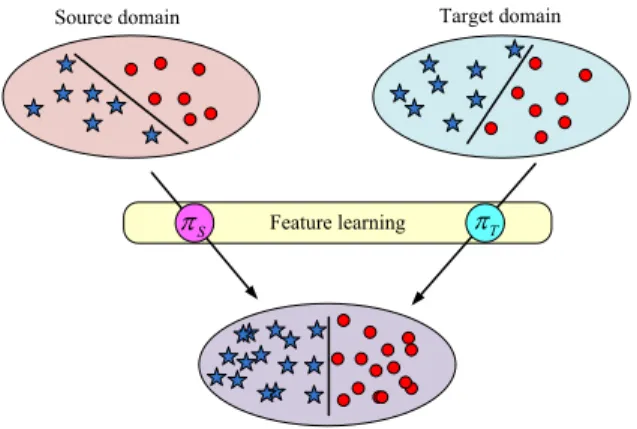
Fig. 3. Feature-level domain adaptation
To solve the problem of spectral shift, domain adaptation is one of the main techniques. The aim of domain adaptation is to reduce the distribution shift between two domains by exploiting their underlying correlations or shared representation components and structures. Domain adaptation has been widely applied in cross-domain learning problems, including image classification, handwritten character recognition, text classification [15], [20], [21]. Classifier level and feature level domain adaptations are two principal approaches. Classifier level methods learn a classifier for target domain from pre-learned classifiers for source domains through the correlation between source and target domains. A cross domain SVM can be learned by a convex combination of loss functions of SVMs in source and target domains [22]. Yang et al [23] proposed to learn a “delta function” from the source and target data, and then added it to the SVM model for domain adaptation. Duan et al [24] imposed a data-dependent regularizer of smoothness into least-squares SVM to enforce the target classifier to share similar decision values with the source domain classifiers. Xu and Sun [25] proposed an Adaboost cross domain classifier in which a new parameter was designed to indicate domain relationship, and the combination of multiple learners was adopted to output the target hypothesis. Instance weighted classifiers try to compensate the differences in marginal/conditional distributions between domains by adaptively weighting instances [26]–[29]. Instance weighting can eliminate the negative effect of the misleading instances that are not compatible with target domain [15]. The weights of instances are usually decided by their prediction confidences during co-training procedure.
Feature level method (also called subspace method in some literature) is more direct and general for domain adaptation. It maps the source and target domain spaces into a common feature subspace where the distribution shift is reduced [30]–[33]. Shown by Fig. 3, feature level domain adaptation is to find feature projections πS(·) andπT(·)so that the distributions of projected featuresP(πS(XS))andP(πT(XT))are similar, and the projected featureπT(XT)is more discriminative [34]. One idea is to represent source and target data on Grassmann manifold, and then use the geodesic path is to obtain intermediate subspaces [30]. Other work adopted kernel method to look for the shared feature representation in a reproducing kernel Hilbert space (RKHS). To this end, Pan et al [35] designed an objective function with two goals, one is minimizing the distance of source and target distributions in the RKHS, and the other is preserving the data variance in each domain.
Another type of feature level domain adaptation is dictionary learning. Dictionary learning on signals and images has attracted tremendous interest in recent years, as signals or images can be more effectively represented in a specific subspace spanned by atoms in a dictionary. In particular, a data-driven dictionary can adapt to input data so its generated new feature space can provide more robust and discriminative data representations for many applications [36]–[38]. In domain adaptation point of view, dictionary learning generates a domain-invariant space which are jointly learned from both source and target data [34]. Dictionary learning based domain adaptation was first used for self-taught learning where the number of labeled training samples is limited but there exist a large amount of unlabeled but related samples. For example, a large amount of unlabeled data can be used to learn a dictionary with K-SVD algorithm, and then the coding coefficients on the dictionary are treated as domain-invariant features [20], [39]. Through this dictionary-based feature representation, classification performance on the target domain can be greatly improved. Ni et al [40] learned an initial dictionary from source data, then the dictionary was gradually updated using target domain information, and finally a dictionary was learned for the target domain. Shekhar et al [41] proposed a robust method for learning a single dictionary to optimally represent both source and target data. In particular, they proved that learning a dictionary on a low-dimensional space reduces the irrelevant information in original features in different domains. Furthermore, the problem of small-training-size in HSI classification goes along with high-dimensionality problem, as HSIs always have hundreds of bands and their transformed feature spaces such as wavelet transformed feature space [42] will have higher dimensions. Therefore, dictionary learning based domain adaptation is a suitable choice for its combination of dimensionality reduction and cross-scene feature extraction. Other properties of this method will be further discussed in the next section.
III. FEATURE LEVEL DOMAIN ADAPTATION FOR CROSS-SCENEHSICLASSIFICATION
Feature level domain adaptation for scene HSI classification can be divided into two steps, i.e., cross-domain feature extraction and classifier training. The first step is to transform the spectral cross-domains of source and target scenes into a shared feature space in which spectral shift can be reduced by extracting their inherent identical structure. Nonnegative matrix factorization (NMF) based dictionary learning is used in this paper to generate the shared feature space. This method has an intrinsic relation with the mixture spectral model of hyperspectral imaging, so it can give a physical interpretation for this shared feature space. The second step is to learn a classifier in the shared feature space with training samples from source scene or from both source and target scenes. In this paper, sparse logistic regression (SRL) is selected as the classifier. SRL combines classifier learning and feature selection into one frame, which selects discriminative features from the shared feature spaces so that spectral shift can be further reduced.
A. Cross-scene feature extraction via multitask NMF based dictionary learning
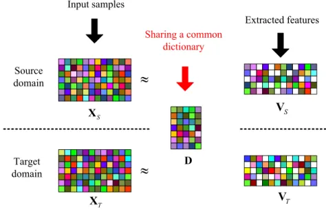
A general assumption for unsupervised domain adaptation is that there exist certain discriminative features shared by both domains [30], [43]. From the dictionary learning based domain adaptation point of view, this assumption implies that samples in source and target domains share a common dictionary on which they can be consistently represented. The representation coefficients on the learned dictionary are utilized as the cross-domain features for
»
D SV
»
TV
Sharing a common dictionary Source domain Target domain SX
TX
Input samples Extracted featuresFig. 4. Feature level domain adaptation via a shared dictionary.
the training and testing samples in different scenes. These new features in the common space not only have less distribution shift between source and target scenes, but also have more discriminative ability between different classes. Here, multitask joint dictionary learning (MTJDL) is proposed for learning a shared dictionary from both source and target domains. The model framework is illustrated in Fig. 4, in which the samples from source and target domains are used to train a shared dictionary, and then the coefficient vectors are taken as the new extracted features. During dictionary learning, the class labels of samples are not considered, i.e. both samples with or without labels can be used for dictionary learning, so this method belongs to unsupervised dictionary learning.
There are several unsupervised dictionary learning algorithms such as method of optimized directions (MOD) [44], K-SVD [45], NMF [46], etc. Among them, NMF has some distinct advantages. NMF can learn a parts-based representation of the data by factorizing a nonnegative matrix into two nonnegative factor matrices. One factor matrix can be seen as a dictionary, and the other is the linear representation on this dictionary. From the view of linear spectral mixture model, two factor matrices decomposed by NMF correspond to the endmembers and the abundances, so NMF and its extensions have been successfully used for hyperspectral unmixing [47]–[50]. In this sense, the learned dictionary by NMF also can be seen as a spectral library consisting of the endmembers in the HSIs being processed. In spite of the potential spectral shift between scenes, the spectra of pixels in different scenes can be approximated by linear combination of endmembers, so dictionary learning based domain adaptation for cross-scene HSI classification can be considered as a problem of learning their common spectral library and then using the corresponding abundances as the new features of pixels. Although the conditions of NMF for dictionary learning is weaker than those for unmixing, for example, the number of endmembers (the size of spectral library) is not required to be estimated accurately, the interpretation of domain adaptation from the mixture model point of view is intuitive and beneficial to interpreting dictionary learning based domain adaptation.
called simultaneous NMF, was first proposed by Badea [51] to extract common gene expression profiles that are shared by colon and pancreatic adenocarcinoma. In the multitask NMF, two or more NMF tasks are bound together by sharing a common factor matrix (i.e., dictionary). When applied to cross-scene HSI data sets, multitask NMF can be considered as a tool to extract a common set of endmembers shared by different but related HSI data sets.
The model of multitask NMF is defined as min D, (vS)i,i=1,2,...,mS, (vT)j,j=1,2,...,mT (mS X i=1 k(xS)i−D(vS)ik 2 2+ mT X j=1 k(xT)j−D(vT)jk 2 2 ) s.t. (vS)i≥0, i= 1,2, . . . , mS, (vT)j≥0, j= 1,2, . . . , mT, (4) where(xS)i∈R n +and(xT)j∈R n
+are the spectral profiles of the pixels in source and target domains, respectively.
D∈Rn+×p is the common dictionary matrix shared between two domains, whose columns are basis atoms. (vS)i and(vT)j are the coefficient vector of (xS)i and(xT)j, respectively. The dictionary size is set smaller than the number of spectral bands, i.e., p < n, thus a dimensional reduction is embedded in feature extraction, which is beneficial to small-training-size classification.
Following solution for the traditional NMF, multiplicative update (MU) algorithm can be used to solve Eq. (4) by an alternating optimization procedure. Eq. (4) can be briefly written as
F(D,VS,VT) =kXS−DVSk2F+kXT−DVTk2F (5)
whereXS = [(xS)1,(xS)2, . . . ,(xS)mS], VS = [(vS)1,(vS)2, . . . ,(vS)mS],XT = [(xT)1,(xT)2, . . . ,(xT)mT],
andVT = [(vT)1,(vT)2, . . . ,(vT)mT]. The partial derivatives ofF with respect toVS,VT andDare calculated
as ∂F ∂VS = 2DTDVS−2DTXS (6) ∂F ∂VT = 2DTDVT −2DTXT (7) ∂F ∂D = 2DVSV T S −XSVST+ 2DVTVTT −XTVTT (8)
Using the Karush-Kuhn-Tucker (KKT) conditions, we set ∂∂FV
S = 0,
∂F ∂VT = 0,
∂F
∂D = 0, and get the MU rules, i.e., VS ←VS~(DTXS)(DTDVS) (9) VT ←VT~(DTXT)(DTDVT) (10) D←D~(XSVTS+XTVTT)(DVSVTS+DVTVTT) (11) After alternatively updatingVS,VT andD, the minimization of objective function Eq. (5) can be achieved. Finally, the extracted high level features (VS andVT) are fed into a suitable classifier for training and prediction.
B. Classification algorithm
After cross-scene feature extraction, many classical classifiers can be applied, such as support vector machine (SVM) [52], neural networks [53], sparse representation [54], et al. Here sparse logistic regression (SLR) is used, which selects a small number of important/discriminative input variables such that the output of a system can be approximately predicted. It can reduce the disturbance of noisy and irrelevant variables, increase the modeling accuracy and robustness, and improve the interpretation of the system. Some simple and fast computational algorithms have been proposed to deal with large-scale problem. Various applications in computer vision, data mining, and signal processing have proven its effectiveness [42]. In the case of cross-scene HSI classification, since multitask NMF based dictionary learning is unsupervised, it does not consider the discrimination for different land cover classes. SRL enables us to select discriminative features from the shared feature space for further reducing distribution shift and increasing classification accuracy.
In the training procedure, the following objective function of SLR is minimized, min
w,c m X i=1
log(1 + exp(−yi(wTvi+c))) +λkwk1 (12) where vi is the feature vector and yi ∈ {1,−1} is the class label of the ith training sample. The optimization algorithm for (12) can be found in [55], [56]. After the coefficients (w, c) are estimated, the classifier works in a probabilistic way to label the input test samplexusing its feature vectorv.
P(y= 1|v) = 1
1 + exp(−(wTv+c)) (13)
For multi-class problem, one-versus-one voting scheme can be utilized.
Multitask NMF based unsupervised learning dictionary can reduce spectral shift, but cannot completely clear it. Therefore, even in a shared feature space, the classifiers for source scene and target scene need to have subtle nuances if we want to reach further improved cross-scene classification. When a few labeled samples are available in target scene, we can train two classifiers for source and target scenes respectively, making them not only have consistency but also preserve their distinct identities. As a multitask version of SLR, multitask SLR (MTSLR) is used to simultaneously train two SLR models with the label samples in source and target scenes respectively, but these two SRL models share a common discriminative feature subset while the non-discriminative features and the features incompatible between two domains are discarded [17]. Different from SRL based cross-scene classifier that trains a single SRL model for both source and target scenes, MTSLR provides two strongly related but little differentiated classifiers for two different scenes, which can further reduce impact of the residuary distribution shift after dictionary learning based feature level domain adaptation.
The objective function of MTSRL is defined as min wS,cS, wT,cT (mS X i=1 log(1 + exp(−(yS)i(w T S(vS)i+cS))) + mT X j=1 log(1 + exp(−(yT)j(wTT(vT)j+cT))) +λk[wS,wT]k2,1 ) (14)
Joint feature selection Source domain Target domain T S
w
SV
=
Sz
( | ) S S P y =1 S Sigmoid function T T w TV
=
Tz
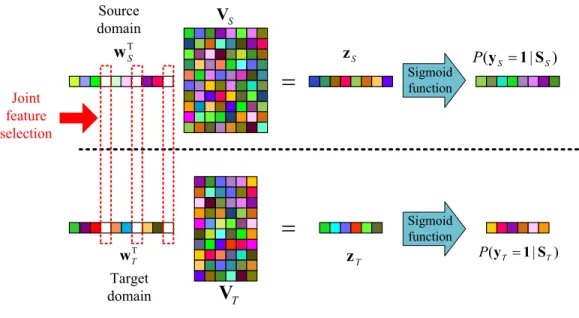
P(yT =1 S| T) Sigmoid functionFig. 5. MTSLR based joint feature selection. TheVSandVT are the MTJDL based features from source and target domains, respectively.
The white elements inwSandwT stand for zero elements.
where(vS)i and(vT)j are the features of training samples in source and target domains obtained by NMF based MTJDL.(yS)iand(yT)j∈ {1,−1}are their corresponding class labels.wS andwT are sparse coefficient vectors, and cS andcT are the corresponding intercept terms. The model framework is shown in Fig. 5 where two SLR models are trained for source and target domains, respectively (see the first and second terms in Eq. (14)). Rather than separately training two SLR models, we bind them by sharing a same sparse structure (or called sparse pattern) in coefficient vectors via`2,1 regularization (the last term in Eq. (14)), which is defined as
k[wS,wT]k2,1= n X i=1 q (wS)2i + (wT)2i. (15)
The regularization parameter λ controls the sparsity level in wS and wT. The MTSLR model completes joint feature selection and training of two classifiers at the same time.
Since the`2,1 norm regularization term in objective function (14) is non-differentiable at certain points, we can
not directly minimize the whole objective function by the basic optimization methods such as gradient descent, etc. One of valid algorithms to solve the non-smooth problem is proximal gradient descent [57]–[59].
We denote the logistic loss functions in source and target domains as
LS(wS, cS) = mS X i=1 log(1 + exp(−(yS)i(w T S(vS)i+cS))) (16) LT(wT, cT) = mT X j=1 log(1 + exp(−(yT)j(wTT(vT)j+cT))) (17) thus the objective function in Eq. (14) is written as
LS(wS, cS) +LT(wT, cT) +λk[wS,wT]k2,1. (18)
1) apply gradient descent on the differentiable part (i.e.,LS+LT) without considering`2,1 regularization;
2) apply proximal operator (or called shrinkage in some literatures) for`2,1 regularization.
The detailed algorithm steps are listed in Algorithm 1. OncewT, cT are obtained, an input test samplex in target scene can be classified in the same way as Eq. (13).
Algorithm 1 Proximal gradient descent for MTSLR
Input:
Input features of training samples from source and target domains VS∈Rn×mS,V
T ∈Rn×mT,
Corresponding class labels yS ∈RmS,y
T ∈RmT,
Regularization parameterλ.
Output:
The coefficient vectors for source and target domains wS ∈ Rn,wT ∈ Rn and the corresponding intercepts
cS ∈R, cT ∈R.
1: Initialize wS =0,wT =0, cS = 0, cT = 0. 2: repeat
3: OptimizeLS andLT with gradient descent:
wS ←wS−α∇wSLS cS ←cS−α∇cSLS
wT ←wT −α∇wTLT cT ←cT −α∇cTLT
whereαis step size obtained by line search.
4: Apply proximal operator to handle`2,1 regularization:
[wS,wT]←arg min W
kW−[wS,wT]k2F+λkWk2,1
which can be solved by shrinkage
W[i] = 1− αλ kU[i]k 2 U[i], U[i] 2> αλ 0, otherwise i= 1,2, . . . , n ,
whereU= [wS,wT]andU[i] is ith row ofU. 5: until convergence is reached.
IV. EXPERIMENTAL RESULTS
In this section, we will validate the proposed cross-scene HSI classification methods on several synthetic and real-world data sets. According to whether the labeled training samples are available in target scene or not, we divide the comparative experiments into two groups. The first group deals with the case that only labeled samples in source scene are available. Following three algorithms are used:
• Source domain SLR (SD-SLR): It trains an SLR model by only using the training samples in the source scene, and then the learned SLR model is directly applied to the testing samples in target scene for prediction. Note that this straightforward scheme does not consider any domain adaptation at all, and therefore is regarded as the baseline when no labeled training sample is available in target scene.
• Transductive support vector machine (TSVM): It is a very popular classifier level domain adaptation method, which handles the transductive learning by retraining [26]. At first, a classifier is trained using only the labeled samples in source scene, and then this classifier is applied to the unlabeled samples to determine their labels in target scene. Second, the unlabeled samples are added to the training set with the assigned labels to update the classifier. Afterwards, several retraining steps are performed in iterations, and each iteration includes reassigning the class labels of unlabeled samples in target scene and retraining the SVM.
• SD-MTJDL-SLR: It is the proposed algorithm in the paper, which learns a shared dictionary by the samples (labeled and unlabeled) in both source and target scenes using multitask NMF based MTJDL model, and then trains an SLR classifier and classifies all testing samples in the new and shared space. As no labeled samples are validate in target scene, the training of SRL only uses the labeled samples in source scene, which is the same as SD-SLR, but the spectral shift in the shared space is less than that in the original spectral space. The other group cope with the setting that there are a relative large amount of labeled samples in source scene and a small number of labeled samples in target scene. Following five algorithms are taken into experimental comparison:
• Target domain SLR (TD-SLR): It only uses the labeled training samples in target scene to train an SLR model in the original spectral feature space, and then it is applied to the testing samples in target scene. This method does not use any information of the source scene, so it is seen as the baseline in the case that the labeled training samples exist in target scene.
• Merge-SLR: It merges all labeled training samples within both source and target scenes into a united training set, then an SLR model is trained with this training set in the original spectral feature space for classification. It does not consider spectral shift between source and target scenes, i.e., domain adaptation is not used. • TD-MTJDL-SLR: Like TD-SLR, it also only use the labeled training samples in target scene, but the feature
extraction is based on MTJDL. It firstly uses multitask NMF to learn a shared dictionary with labeled and unlabeled samples in both source and target scene, and then trains an SLR classifier on this space with just the labeled samples in target scene.
• Merge-MTJDL-SLR: It is our proposed method in the paper. The only difference with TD-MTJDL-SLR is that Merge-MTJDL-SL uses both training samples in source and target scenes.
TABLE II
THE SPECTRAL SIGNATURES FOR GENERATING THE SYNTHETIC DATA
Source Target
Class
1
(x1
S)1=Douglas-Fir YNP-DF-1 (α1S)1∼ N(0.2,0.052) (x1T)1=Douglas-Fir YNP-DF-2 (α1T)1∼ N(0.3,0.052)
(x1
S)2=Espruce-Sfir YNP-SF-2 (α1S)2∼ N(0.15,0.052) (x1T)2=Espruce-Sfir YNP-SF-3 (α1T)2∼ N(0.2,0.052)
(x1
S)3=Grass-Fescue-Wheatg YNP-FW-1 (α1S)3∼ N(0.2,0.052) (x1T)3=Grass-Fescue-Wheatg YNP-FW-2 (α1T)3∼ N(0.1,0.052)
(x1
S)4=Lodgepole-Pine YNP-LP0-MOD (α1S)4∼ N(0.25,0.052) (x1T)4=Lodgepole-Pine YNP-LP0-VIG (α1T)4∼ N(0.3,0.052)
(x1
S)5=Lodgepole-Pine YNP-LP1-A (α1S)5∼ N(0.2,0.052) (x1T)5=Lodgepole-Pine YNP-LP1-B (α1T)5∼ N(0.1,0.052)
Class
2
(x2
S)1=Lodgepole-Pine YNP-LP2-A (α2S)1∼ N(0.3,0.052) (x2T)1=Lodgepole-Pine YNP-LP2-B (α2T)1∼ N(0.2,0.052)
(x2
S)2=Sagebrush YNP-SS-1 (α2S)2∼ N(0.25,0.052) (x2T)2=Sagebrush YNP-SS-2 (α2T)2∼ N(0.2,0.052)
(x2
S)3=Wetland YNP-WT-1 (α2S)3∼ N(0.1,0.052) (x2T)3=Wetland YNP-WT-2 (α2T)3∼ N(0.2,0.052)
(x2
S)4=Whitebark-Pine YNP-WB-1 (α2S)4∼ N(0.15,0.052) (x2T)4=Whitebark-Pine YNP-WB-2 (α2T)4∼ N(0.3,0.052)
(x2
S)5=Lodgepole-Pine YNP-LP3-A (α2S)5∼ N(0.2,0.052) (x2T)5=Lodgepole-Pine YNP-LP3-B (α2T)5∼ N(0.1,0.052)
• MTJDL-MTSLR: It is proposed in the paper to further improve feature level domain adaptation by training two SRL models for source and target scenes respectively in a structured constraint. Compared with Merge-MTJDL-SLR, MTJDL-MTSLR not only reduces spectral shift with unsupervised dictionary learning, bur also considers the residual spectral shift in a supervised classifier learning procedure.
The main reason of selecting the above methods for experiments is to find: 1) the impact of spectral shift on cross-scene HSI classification; 2) the usefulness of source information to target scene classification; 3) the effect of the proposed domain adaptation methods.
Model parameter setting is a critical factor to ensure fair comparisons. For SD-SLR, TD-SLR and Merge-SLR, we test their SLR model with parameterλ∈ {10−1,10−2,10−3, . . . ,10−7}, and select the value of parameter with the highest classification accuracy for comparison. For TSVM, similar to the default settings of SVMlight, the parameter C is adaptively estimated [60]. Two parameters of SD-MTJDL-SLR, TD-MTJDL-SLR and MTJDL-MTSLR are set asp∈ {5,6, . . . ,30}, andλ∈ {10−1,10−2, . . . ,10−7}. In the comparison, we select the best parameter values
by cross-validation.
A. Experiments on synthetic data
To give a quantitative analysis on synthetic data, we generate the synthetic data from the USGS digital spectral library [61]. Several factors are taken into consideration for preferably simulating the real situation of cross-scene HSI classification: 1) There is spectral shift between source and target scenes, i.e.,P(XS)6=P(XT)andP(yS|XS)6=
P(yT|XT). 2) There is similarity of spectral distribution for the same class between source and target scenes, i.e., the same land cover class consists of the same or similar materials and the corresponding distributions in different scenes. 3) There exists discrimination of spectral distributions between different classes in both of source and target scenes. To ensure the difficulty of cross-scene classification, the separability between different classes is not set high.
Band
10
20
30
40
Reflectance
0.1
0.15
0.2
0.25
0.3
0.35
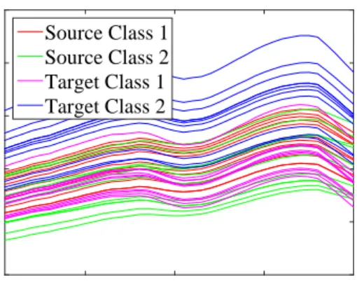
Source Class 1 Source Class 2 Target Class 1 Target Class 2Fig. 6. Spectral profiles of some randomly selected samples in synthetic data.
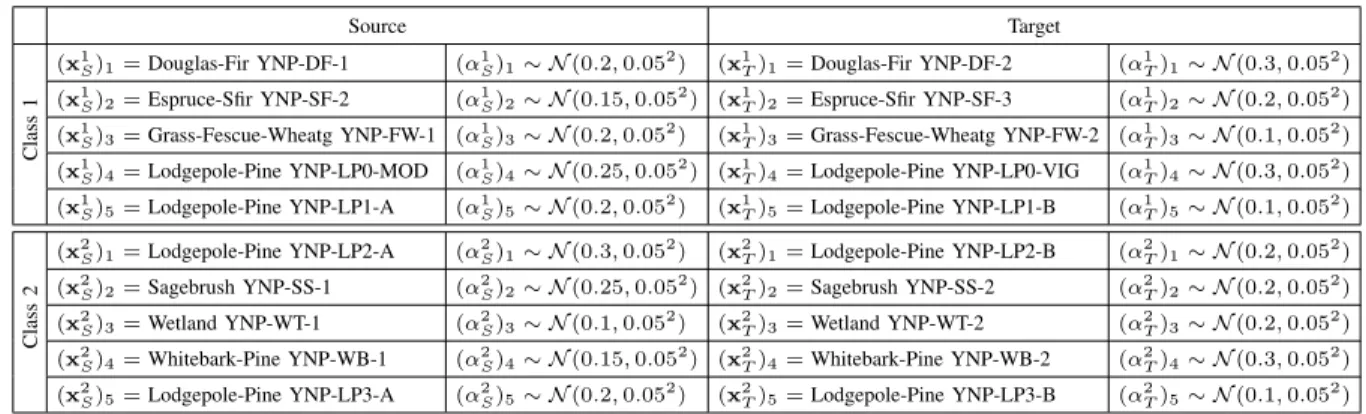
• We select twenty spectral profiles from the USGS library, which are categorized into four groups, and each contains five spectral profiles of five materials (or called endmembers in linear spectral mixture model). These four groups are used to separatively generate two classes within two scenes, i.e., “Source Class 1”, “Source Class 2”, “Target Class 1”, “Target Class 2”.
• For each class, we use similar endmembers for source and target scenes to ensure that a land cover class consists of similar materials, e.g.,(x1
S)1=Douglas-Fir YNP-DF-1 is very similar to(x1T)1=Douglas-Fir YNP-DF-2,
which are both sub-categories of Douglas-Fir.
• Each class is generated by linear combination of five endmembers in the corresponding group, e.g., a sample of class 1 in source domain can be generated by x1
S =
5
P i=1
(α1
S)i(x1S)i (see Table II)
• The abundances of each sample in a class is generated randomly by Gaussian distribution. To make reasonable spectral shift between source and target domains, the distribution of abundances vary between source and target scenes (see Table II), e.g.(α1S)1∼ N(0.1,0.052)and(α1T)1∼ N(0.3,0.052)have different mean values.
• To make the classification more challenging, we use a band subset containing 40 bands (bands 41–80 from the original data), which decreases the discrimination between classes.
In summary, the spectral shift in the synthetic data is rooted in the different but similar endmembers and the different abundances when generating different samples of a class in source and target domains. Spectral profiles of some randomly selected samples are plotted in Fig. 6.
In experiments on synthetic data, the number of source domain training samples is set to 500 per class (thus 1000 in total). In the experiments where labeled training samples are available in target domain, we select 5 samples per class (thus 10 in total). Whether training samples are available in target domain or not, 1000 testing samples per class are drawn from target domain to evaluate the classification performance. In the following experiments, overall accuracy (OA), average accuracy (AA) and kappa coefficient (κ) are utilized as performance criteria. Note that since two classes have the same number of test samples, OA=AA always holds for synthetic data.
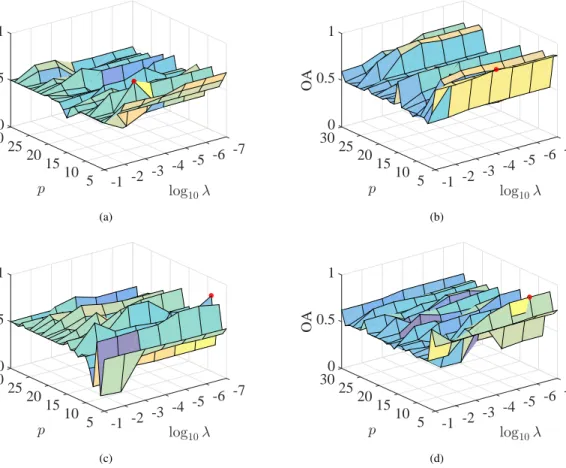
0 30 25 0.5 -7 OA -6 20 p -5 log10λ 15 1 -4 -3 10 -2 5 -1 (a) 0 30 25 0.5 -7 OA -6 20 p -5 log10λ 15 1 -4 -3 10 -2 5 -1 (b) 0 30 25 0.5 -7 OA -6 20 p -5 log10λ 15 1 -4 -3 10 -2 5 -1 (c) 0 30 25 0.5 -7 OA -6 20 p -5 log10λ 15 1 -4 -3 10 -2 5 -1 (d)
Fig. 7. OA versepandλ. (a) SD-MTJDL-SLR, and its best OA= 0.7970is achieved withp= 6andλ= 10−3. (b) TD-MTJDL-SLR, its best OA= 0.8990is achieved withp= 5andλ= 10−4. (c) MTJDL-Merge-SLR, its best OA= 0.8115is achieved withp= 9and λ= 10−7. d) MTJDL-MTSLR, its best OA= 0.9695is achieved withp= 6andλ= 10−3.
based dictionary learning, the dictionary size p is an important parameter. For SLR and MTSLR, there is only one parameterλwhich controls the sparsity level. Therefore, Fig. 7 shows that the classification accuracy changes with different values ofpandλfor SD-MTJDL-SLR, TD-MTJDL-SLR, Merge-MTJDL-SLR and MTJDL-MTSLR methods, where the range ofpis from 5 to 30, andλfrom10−7 to10−1. The red point represents the parameter
setting that archives the best OA.
It is found that a dictionary with small size (p) can better reduce spectral shift, which is consistent with the conclusion made in [41]. Although the best values of λare very different for these four methods, it can also be seen thatλ should be set to a small value to reach a high accuracy. Methods on how to determine the degree of sparsity have been proposed in the literature, which are beyond the scope of our paper.
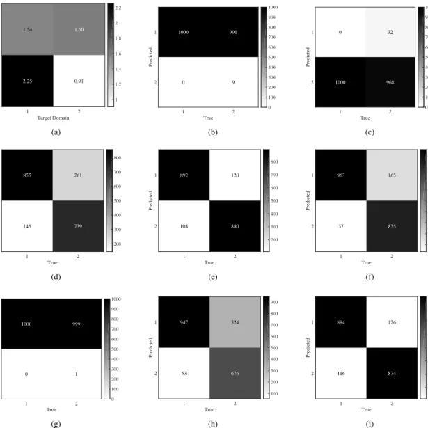
Then we give the comparative classification results in Table III, where the first three rows correspond to the case that the training samples in target domain is not available, while the last five rows are under the condition that both a limited number of training samples and a relative large amount of training ones are available in target and source domains, respectively. Their CSMSAD matrix along with the confusion matrices of classification are illustrated in Fig. 8. In the case when no training sample exists in target domain, SD-SLR classifies all the testing samples in
TABLE III
CLASSIFICATION ACCURACY ON SYNTHETIC DATA
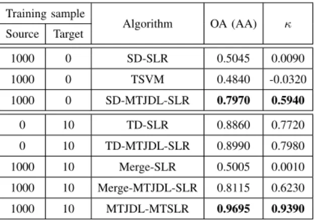
Training sample Algorithm OA (AA) κ Source Target 1000 0 SD-SLR 0.5045 0.0090 1000 0 TSVM 0.4840 -0.0320 1000 0 SD-MTJDL-SLR 0.7970 0.5940 0 10 TD-SLR 0.8860 0.7720 0 10 TD-MTJDL-SLR 0.8990 0.7980 1000 10 Merge-SLR 0.5005 0.0010 1000 10 Merge-MTJDL-SLR 0.8115 0.6230 1000 10 MTJDL-MTSLR 0.9695 0.9390
the target domain Class 1 (see Fig. 8(b)), resulting in a very poor OA/AA of0.5045. This indicates that directly training a classifier in source domain and applying it to target domain is not a good choice due to spectral shift. For TSVM, though knowledge transfer is considered, more testing samples are misclassified (see Fig. 8(c)), i.e., its classification accuracy is even worse than SD-SLR. This is caused by the overlapped sample distribution between “Source Class 2” and “Target Class 1” (see Fig. 6). Compared with SD-SLR and TSVM, SD-MTJDL-SLR has a much higher classification accuracy, which is also illustrated in Fig. 8(d). This indicates the proposed MTJDL based domain adaptation can greatly reduce spectral shift and improve the cross-scene classification performance. When some training samples in target domain are also available, the situation becomes to be more complicated. Both TD-SLR and Merge-SLR are based on the original spectral features, the former only uses the target domain training samples, and the latter uses all training samples in two domains. It can be obviously seen that TD-SLR is much better than Merge-SLR, i.e., the training samples in source domain play a negative effort. It again indicates that spectral shift make a classifier directly learned from just source domain or both source and target domains is not valid to target domain classification. Their corresponding versions in the shared feature space, TD-MTJDL-SLR and TD-MTJDL-SLR, also reflect the same fact in the experiments, but the classification accuracies of TD-MTJDL-SLR and TD-MTJDL-SLR are higher than those of TD-SLR and Merge-SLR respectively, especially the improvement of TD-MTJDL-SLR is very significant when compared with TD-SLR. This is a further evidence that the proposed feature level domain adaptation is useful to reduce spectral shift, but it also indicates that spectral shift is not totally cleared. Our MTJDL-MTSLR method not only considers their consistency in the shared spare, but their difference (remained distribution shift) as well, so it achieve the best classification performance.
B. Experiments on real-world data
Now we turn to the real-world cross-scene HSI classification. Three cross-scene HSI datasets are used, including Indiana scenes, Pavia scenes and Shanghai-Hanghzou scenes.
The whole Indiana scene was captured by AVIRIS sensor on June 12, 1992 during a flight over 25×6 mile portion of Northwest Tippecanoe County, Indiana [62]. The size of the original whole HSI data is614×2166×220,
1.54 2.25 1.60 0.91 1 2 Target Domain 1 2 Source Domain 1 1.2 1.4 1.6 1.8 2 2.2 (a) 1000 0 991 9 1 2 True 1 2 Predicted 0 100 200 300 400 500 600 700 800 900 1000 (b) 0 1000 32 968 1 2 True 1 2 Predicted 0 100 200 300 400 500 600 700 800 900 1000 (c) 855 145 261 739 1 2 True 1 2 Predicted 200 300 400 500 600 700 800 (d) 892 108 120 880 1 2 True 1 2 Predicted 200 300 400 500 600 700 800 (e) 963 37 165 835 1 2 True 1 2 Predicted 100 200 300 400 500 600 700 800 900 (f) 1000 0 999 1 1 2 True 1 2 Predicted 0 100 200 300 400 500 600 700 800 900 1000 (g) 947 53 324 676 1 2 True 1 2 Predicted 100 200 300 400 500 600 700 800 900 (h) 884 116 126 874 1 2 True 1 2 Predicted 200 300 400 500 600 700 800 (i)
Fig. 8. CSMSAD matrix and confusion matrices of synthetic data. (a) CSMSAD matrix. (b) confusion matrix of SD-SLR. (c) confusion matrix of TSVM. (d) confusion matrix of SD-MTJDL-SLR. (e) confusion matrix of TD-SLR. (f) confusion matrix of TD-MTJDL-SLR (g) confusion matrix of Merge-SLR. (h) confusion matrix of Merge-MTJDL-SLR. (i) confusion matrix of MTJDL-MTSLR.
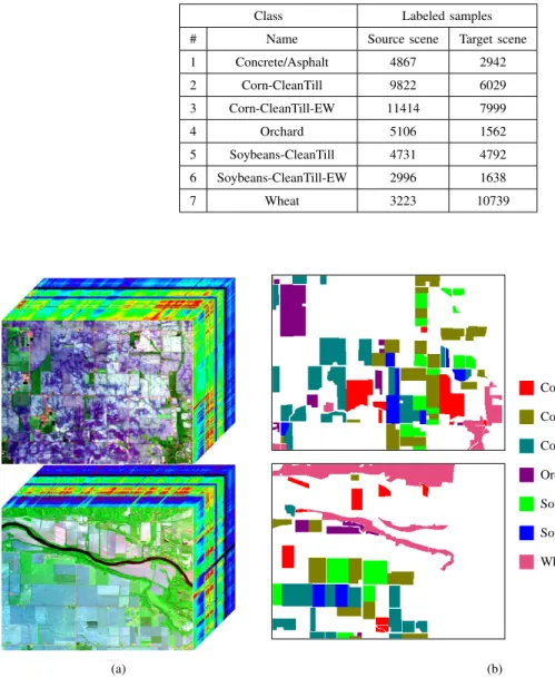
where the last dimension is the number of bands. Band 120 of the original whole scene is displayed in Fig. 1. We select two spatial disjointed subsets (the regions in the red boxes) as source and target scenes, respectively. Both source and target scenes are sized 400×300×220. We select seven land cover classes shared by both scenes for classification, which are listed in Table IV. The data cubes and corresponding ground truth maps of two sub-scenes are illustrated in Fig. 9.
In the experiments on Indiana data, the number of source domain training samples is set to 180 per class (thus 1260 in total). The number of target domain training samples is set to 20 per class (thus 140 in total) in the case when the training samples are available in target scene. The remaining labeled samples in target scene are used as testing samples to evaluate the classification performance. All experiments are conducted in the same way as
TABLE IV
NUMBER OF LABELED SAMPLES IN EACH LAND COVER CLASS WITHININDIANA SCENES
Class Labeled samples # Name Source scene Target scene 1 Concrete/Asphalt 4867 2942 2 Corn-CleanTill 9822 6029 3 Corn-CleanTill-EW 11414 7999 4 Orchard 5106 1562 5 Soybeans-CleanTill 4731 4792 6 Soybeans-CleanTill-EW 2996 1638 7 Wheat 3223 10739 (a) Concrete/Asphalt Corn−CleanTill Corn−CleanTill−EW Orchard Soybeans−CleanTill Soybeans−CleanTill−EW Wheat (b)
Fig. 9. Source and target scenes in Indiana datasets. The upper row is the source scene, while the lower row is the target scene. (a) Data cubes. (b) Ground truth maps.
in synthetic data. The accuracies obtained from different algorithms are listed in Table V. The CSMSAD matrix and their confusion matrices are shown in Fig. 10. Like the results on the synthetic data, the results on Indiana data also demonstrate that the proposed multitask NMF based dictionary learning is a good choice for feature level domain adaptation, and MTSLR can further reduce the impact of distribution shift after domain adaptation. SD-MTJDL-SLR and MTJDL-MTSLR achieve the highest accuracies respectively when the training samples in target are available or not. It should be noted that the effect of domain adaptation is different for different classes, which is due to the complicated relation between classes in spectral distribution. For example, comparing Fig. 10(d) with Fig. 10(b), we find that SD-MTJDL-SLR greatly improves the classification accuracy of class 3, but it fails
TABLE V
CLASSIFICATION ACCURACY ONINDIANA DATA
Training sample Algorithm OA AA κ Source Target 1260 0 SD-SLR 0.4794 0.4155 0.3617 1260 0 TSVM 0.3919 0.3382 0.2742 1260 0 SD-MTJDL-SLR 0.5134 0.4351 0.3845 0 140 TD-SLR 0.5109 0.4931 0.4031 0 140 TD-MTJDL-SLR 0.5852 0.5762 0.4918 1260 140 Merge-SLR 0.5056 0.4541 0.3973 1260 140 MTJDL-Merge-SLR 0.5196 0.4591 0.3950 1260 140 MTJDL-MTSLR 0.5975 0.5861 0.5059
to work well on class 1.
The second real HSI data are acquired from the hyperspectral airborne sensor DAIS over the urban areas of Pavia City, Italy1, in which the Pavia University image is selected as the source scene whose size is 243×243×72,
and the Pavia Center image is selected as the target scene whose size is400×400×72. Six common land cover classes are considered for the cross-scene classification, which are listed in Table VI. The data cubes and ground truth maps of both scenes are displayed in Fig. 11. In the experiments on Pavia data, the number of source domain training samples is set to 180 per class, while the number of target domain training samples is set to 20 per class in the case of the training samples in target domain are also available. The classification results of various algorithms are presented in Table VII. The CSMSAD matrix of Pavia data and the confusion matrices produced by different algorithms are shown in Fig. 12. The classification results indicate if the training samples in target scene cannot be obtained, the proposed multitask NMF is an excellent domain adaptation method for cross-scene HSI classification, and if a limited number of the training samples in target scene are available, the combination of MTJDL and MTSLR is an effective technique, i.e., level feature and classifier level domain adaptation should be used together. Another conclusion is that even only very limited number of training samples exist in target scene, they play an important role in the cross-scene classification. Comparing the accuracies of SD-MTJDL-SLR and MTJDL-MTSLR, we can see only a little amount of training samples in target scene (120 per class) bring more than 10%gain in OA, AA, andκ.
Thirdly, we test the proposed methods on Shanghai-Hangzhou scenes. Shanghai and Hangzhou HSI datasets were both captured by EO-1 Hyperion hyperspectral sensor. The Hyperion sensor provides 220 spectral bands, but after removing bad bands, 198 bands remain. Shanghai data set was acquired in Apr. 1st 2002 over Shanghai that is the largest city of China and locates in the east of China. We select an image with the size of1600×230×198, which covers some urban and rural areas of Shanghai, including roads, buildings, plants and the water bodies of the Yangtze River and the Huangpu River. Hangzhou data set was captured in Nov. 2nd 2002 over Hangzhou that
1.48 1.56 1.51 1.98 1.51 1.52 2.01 1.39 1.35 1.29 2.02 1.28 1.28 2.09 1.44 1.41 1.34 2.09 1.33 1.32 2.16 1.80 1.85 1.92 0.95 1.93 1.94 0.89 1.38 1.33 1.26 2.10 1.24 1.23 2.20 1.46 1.40 1.32 2.15 1.31 1.28 2.25 1.67 1.67 1.77 0.76 1.78 1.81 0.59 1 2 3 4 5 6 7 Target Domain 1 2 3 4 5 6 7 Source Domain 0.6 0.8 1 1.2 1.4 1.6 1.8 2 2.2 (a) 1894 37 790 124 25 24 28 3341 57 2170 403 0 24 14 3657 140 3670 343 136 30 3 50 2 0 1301 0 0 189 2304 15 2261 176 0 16 0 343 2 1214 54 0 5 0 193 63 0 288 53 0 10122 1 2 3 4 5 6 7 True 1 2 3 4 5 6 7 Predicted 0 1000 2000 3000 4000 5000 6000 7000 8000 9000 10000 (b) 161 120 2 25 542 1033 1039 536 953 68 29 1089 3106 228 741 1335 51 23 1695 4080 54 23 1 5 184 0 0 1329 27 295 4 0 544 3898 4 10 80 13 1 7 1506 1 8 1 1 147 26 0 10536 1 2 3 4 5 6 7 True 1 2 3 4 5 6 7 Predicted 0 1000 2000 3000 4000 5000 6000 7000 8000 9000 10000 (c) 105 1113 1545 88 17 19 35 669 110 4814 401 1 0 14 787 149 6448 185 111 292 7 7 2 3 1404 0 0 126 120 0 4499 153 0 0 0 6 0 1551 61 0 0 0 39 208 21 251 9 0 10191 1 2 3 4 5 6 7 True 1 2 3 4 5 6 7 Predicted 0 1000 2000 3000 4000 5000 6000 7000 8000 9000 10000 (d) 1366 395 493 28 442 173 25 843 1813 1359 10 1277 681 26 1058 1778 1557 21 2188 1363 14 4 4 0 1470 2 0 62 504 1090 1122 0 1389 667 0 90 294 352 0 393 489 0 197 30 4 395 8 1 10084 1 2 3 4 5 6 7 True 1 2 3 4 5 6 7 Predicted 0 1000 2000 3000 4000 5000 6000 7000 8000 9000 10000 (e) 1575 308 590 7 284 129 29 466 3219 778 10 649 848 39 631 2662 2033 15 1614 1000 24 0 22 0 1378 0 0 142 27 1462 668 0 1523 1092 0 2 272 183 0 309 852 0 167 67 0 250 1 2 10232 1 2 3 4 5 6 7 True 1 2 3 4 5 6 7 Predicted 0 1000 2000 3000 4000 5000 6000 7000 8000 9000 10000 (f) 1352 296 604 133 231 259 47 1636 1118 1741 451 534 503 26 2421 1013 2543 436 420 1138 8 47 3 0 1281 0 0 211 672 371 1399 287 1223 820 0 212 105 815 117 86 283 0 153 29 0 296 62 0 10179 1 2 3 4 5 6 7 True 1 2 3 4 5 6 7 Predicted 0 1000 2000 3000 4000 5000 6000 7000 8000 9000 10000 (g) 37 910 1903 18 0 33 21 396 60 5517 14 2 0 20 566 117 6828 19 378 60 11 6 10 72 1360 0 0 94 16 0 4755 0 0 1 0 1 0 1617 0 0 0 0 36 199 37 255 0 0 10192 1 2 3 4 5 6 7 True 1 2 3 4 5 6 7 Predicted 0 1000 2000 3000 4000 5000 6000 7000 8000 9000 10000 (h) 1550 368 421 54 326 171 32 707 2164 1453 43 1086 524 32 854 2210 1921 32 1904 1042 16 3 1 0 1447 1 0 90 405 1098 1324 5 1345 595 0 55 256 315 0 384 608 0 180 23 0 467 1 0 10048 1 2 3 4 5 6 7 True 1 2 3 4 5 6 7 Predicted 0 1000 2000 3000 4000 5000 6000 7000 8000 9000 10000 (i)
Fig. 10. CSMSAD matrix and confusion matrices of Indiana data. (a) CSMSAD matrix. (b) confusion matrix of SD-SLR. (c) confusion matrix of TSVM. (d) confusion matrix of SD-MTJDL-SLR. (e) confusion matrix of TD-SLR. (f) confusion matrix of TD-MTJDL-SLR (g) confusion matrix of Merge-SLR. (h) confusion matrix of Merge-MTJDL-SLR. (i) confusion matrix of MTJDL-MTSLR.
TABLE VI
NUMBER OF LABELED SAMPLES IN EACH LAND COVER CLASS WITHINPAVIA SCENES
Class Labeled samples # Name Source scene Target scene
1 Trees 266 2424 2 Asphalt 266 1704 3 Parking lot 265 287 4 Bitumen 206 685 5 Meadow 273 1251 6 Soil 213 1475
(a) Trees Asphalt Parking lot Bitumen Meadow Soil (b)
Fig. 11. Source and target scenes in Pavia datasets. The upper one is the source scene (Pavia University), while the lower one is the target scene (Pavia Center). (a) Data cubes. (b) Ground truth maps.
TABLE VII
CLASSIFICATION ACCURACY ONPAVIA DATA
Training sample Algorithm OA AA κ Source Target 1080 0 SD-SLR 0.7434 0.7154 0.6752 1080 0 TSVM 0.6121 0.6150 0.5306 1080 0 SD-MTJDL-SLR 0.8352 0.8130 0.7906 0 120 TD-SLR 0.9465 0.9498 0.9323 0 120 TD-MTJDL-SLR 0.9472 0.9512 0.9331 1080 120 Merge-SLR 0.8281 0.8137 0.7829 1080 120 MTJDL-Merge-SLR 0.8428 0.8294 0.8006 1080 120 MTJDL-MTSLR 0.9507 0.9566 0.9376
0.51 1.41 2.40 1.94 0.99 2.13 1.46 0.81 1.80 1.02 2.04 2.17 2.53 1.75 0.67 1.26 2.09 1.08 1.95 0.94 1.41 0.74 2.40 1.85 0.81 1.98 2.06 2.38 0.56 1.58 2.12 2.01 1.13 1.64 1.61 0.91 1 2 3 4 5 6 Target Domain 1 2 3 4 5 6 Source Domain 0.6 0.8 1 1.2 1.4 1.6 1.8 2 2.2 2.4 (a) 2365 0 0 3 36 0 24 1182 45 433 0 0 0 0 159 82 0 26 0 17 0 648 0 0 350 0 0 0 734 147 6 0 83 42 683 641 1 2 3 4 5 6 True 1 2 3 4 5 6 Predicted 0 500 1000 1500 2000 (b) 2310 1 0 0 93 0 26 77 17 1562 0 2 0 0 127 128 0 12 0 0 0 665 0 0 26 0 0 0 1205 0 2 5 85 899 131 333 1 2 3 4 5 6 True 1 2 3 4 5 6 Predicted 0 500 1000 1500 2000 (c) 2361 5 0 0 38 0 7 1447 99 131 0 0 0 7 210 31 0 19 0 84 5 576 0 0 288 0 0 0 942 1 5 4 145 3 398 900 1 2 3 4 5 6 True 1 2 3 4 5 6 Predicted 0 500 1000 1500 2000 (d) 2320 0 0 0 84 0 2 1615 49 10 0 8 0 2 257 1 0 7 0 14 5 646 0 0 3 0 0 0 1199 29 0 20 114 4 60 1257 1 2 3 4 5 6 True 1 2 3 4 5 6 Predicted 0 500 1000 1500 2000 (e) 2310 20 0 1 73 0 3 1608 41 17 3 12 0 5 262 0 0 0 0 30 1 634 0 0 24 0 0 0 1190 17 0 4 118 2 36 1295 1 2 3 4 5 6 True 1 2 3 4 5 6 Predicted 0 500 1000 1500 2000 (f) 2363 2 0 3 34 2 22 1384 49 229 0 0 0 1 185 66 0 15 0 12 1 652 0 0 119 0 0 0 1079 33 10 2 113 16 596 718 1 2 3 4 5 6 True 1 2 3 4 5 6 Predicted 0 500 1000 1500 2000 (g) 2349 8 0 0 47 0 7 1440 111 126 0 0 0 7 215 23 0 22 0 85 8 572 0 0 250 0 0 0 979 2 5 4 161 2 343 940 1 2 3 4 5 6 True 1 2 3 4 5 6 Predicted 0 500 1000 1500 2000 (h) 2337 0 0 0 67 0 2 1593 60 20 0 9 0 0 261 0 0 6 0 19 1 645 0 0 10 0 0 0 1205 16 0 8 114 8 58 1267 1 2 3 4 5 6 True 1 2 3 4 5 6 Predicted 0 500 1000 1500 2000 (i)
Fig. 12. CSMSAD matrix and confusion matrices of Pavia data. (a) CSMSAD matrix. (b) confusion matrix of SD-SLR. (c) confusion matrix of TSVM. (d) confusion matrix of SD-MTJDL-SLR. (e) confusion matrix of TD-SLR. (f) confusion matrix of TD-MTJDL-SLR (g) confusion matrix of Merge-SLR. (h) confusion matrix of Merge-MTJDL-SLR. (i) confusion matrix of MTJDL-MTSLR.
is the provincial capital of Zhejiang. Hangzhou is also in the east of China, about 170 kilometers far away form Shanghai. A subset with the size of590×230×198is selected from Hanghzou data set. Like the image of Shanghai, Hangzhou image also covers urban and rural areas, including roads, buildings, plants and the water bodies of the West Lake and the Qiantang River. Three land cover classes are labeled for Shanghai and Hangzhou HSIs with the aid of ENVI software. The name of land cover classes and the number of labeled samples are listed in Table VIII. The data cubes and ground truth maps of both scenes are displayed in Fig. 13.
We use Shanghai image as source scene and its number of training samples is set to be 180 per class, while Hangzhou image is used as target scene and the number of target domain training samples is set to 20 per class if available. The experiment results are shown in Table IX and Fig. 14. Different from the results on other data sets, TSVM has a positive effect of improving OA from 0.3264 to0.8277in Shanghai-Hangzhou data. However,
(a)
Water
Ground/Building Plant
(b)
Fig. 13. Source and target scenes in Shanghai-Hangzhou datasets. The upper one is the source scene (Shanghai), while the lower one is the target scene (Hangzhou). (a) Data cubes. (b) Ground truth maps.
TABLE VIII
NUMBER OF LABELED SAMPLES IN EACH LAND COVER CLASS WITHINSHANGHAI-HANGZHOU SCENES
Class Labeled samples # Name Source scene Target scene
1 Water 123123 18043
2 Land/Building 161689 77450
3 Plant 83188 40207
the proposed MTJDL-SLR achieves a higher OA of 0.8933, and the proposed MTJDL-MTSLR has the highest accuracy when the training samples in target scene are available.
Cross-scene classification is important in real applications. From the above experiments, it is concluded that domain adaptation is necessary when labeled samples in source scene are used to help training a classifier for target scene.
0.74 1.10 1.40 1.88 1.75 1.71 2.06 1.79 1.52 1 2 3 Target Domain 1 2 3 Source Domain 0.8 1 1.2 1.4 1.6 1.8 2 (a) 18023 0 0 51210 26220 0 1553 38599 35 1 2 3 True 1 2 3 Predicted 0 0.5 1 1.5 2 2.5 3 3.5 4 4.5 5 ×10⁴ (b) 16257 1766 0 2477 57464 17489 0 1636 38551 1 2 3 True 1 2 3 Predicted 0 1 2 3 4 5 ×10⁴ (c) 16078 1945 0 150 66356 10924 0 1451 38736 1 2 3 True 1 2 3 Predicted 0 1 2 3 4 5 6 ×10⁴ (d) 17174 849 0 4755 68756 3919 1 2119 38067 1 2 3 True 1 2 3 Predicted 0 1 2 3 4 5 6 ×10⁴ (e) 17736 287 0 4172 70945 2313 4 1227 38956 1 2 3 True 1 2 3 Predicted 0 1 2 3 4 5 6 7 ×10⁴ (f) 17998 25 0 4152 70052 3226 0 3454 36733 1 2 3 True 1 2 3 Predicted 0 1 2 3 4 5 6 7 ×10⁴ (g) 17488 535 0 1054 72070 4306 0 4318 35869 1 2 3 True 1 2 3 Predicted 0 1 2 3 4 5 6 7 ×10⁴ (h) 17089 934 0 473 76584 373 0 2672 37515 1 2 3 True 1 2 3 Predicted 0 1 2 3 4 5 6 7 ×10⁴ (i)
Fig. 14. CSMSAD matrix and confusion matrices of Shanghai-Hangzhou data. (a) CSMSAD matrix. (b) confusion matrix of SD-SLR. (c) confusion matrix of TSVM. (d) confusion matrix of SD-MTJDL-SLR. (e) confusion matrix of TD-SLR. (f) confusion matrix of TD-MTJDL-SLR (g) confusion matrix of Merge-SLR. (h) confusion matrix of Merge-MTJDL-SLR. (i) confusion matrix of MTJDL-MTSLR.
classification. The SSI values of a synthetic HSI data set and three real HSI data sets are calculated in Table X. The larger the value of SSI, the larger the degree of spectral shift. In other words, the larger the value of SSI, the more necessary of domain adaptation. Shanghai-Hangzhou data set has the largest SSI, so domain adaptation can play a more important role. The classification results support this judgment, because the SRL classifier with dictionary learning based domain adaptation (SD-MTJDL-SLR) increases OA from 0.3264(obtained by SD-SLR) to0.8933 when the training samples in target scene are unavailable. Therefore, SSI is a reasonable measurement to estimate spectral shift.
TABLE IX
CLASSIFICATION ACCURACY ONSHANGHAI-HANGZHOU DATA
Training sample Algorithm OA AA κ Source Target 540 0 SD-SLR 0.3264 0.4465 -0.0240 540 0 TSVM 0.8277 0.8678 0.7143 540 0 SD-MTJDL-SLR 0.8933 0.9043 0.8167 0 60 TD-SLR 0.9142 0.9294 0.8533 0 60 TD-MTJDL-SLR 0.9410 0.9566 0.8989 540 60 Merge-SLR 0.9200 0.9391 0.8624 540 60 Merge-MTJDL-SLR 0.9247 0.9334 0.8680 540 60 MTJDL-MTSLR 0.9570 0.9615 0.9250 TABLE X
SSIVALUES OF DIFFERENT DATASETS
Dataset SSI Synthetic 0.8125 Indiana 0.7942 Pavia 0.5359 Shanghai-Hangzhou 0.8592 V. CONCLUSION
In this paper, we discuss the problem of cross-scene HSI classification. The main challenge of cross-scene classification is spectral shift between different scenes. Multitask NMF based dictionary learning for feature level domain adaptation is proposed to reduce spectral shift by transforming the spectral feature spaces of source and target scenes into a new shared space. Feature level domain adaptation is independent on the specific classifier. Compared with classifier level domain adaptation, it is more flexible and general-purpose. In particular, multitask NMF based dictionary learning has close relation with spectral unmixing under linear spectral mixture model, making its physical interpretation clear. After the new features of samples in source and target scenes are extracted, SLR is chosen as the classifier as it can select a small subset of features with high discriminative power, which can further reduce spectral shift and remedy the shortcoming of unsupervised dictionary learning that no class information is taken into account. Moreover, if a few labeled samples are available in target scene, instead of SLR that trains a single classifier for both source and target scenes, MTSLR is proposed to simultaneously train two classifiers respectively for source and target scene by`2,1 norm regularization based joint structure constraint. MTSLR can deal with the
residual spectral shift between source and target scenes to improve cross-scene classification performance. It should be noted that this paper is a preliminary work for cross-scene classification that is a new research problem for HSI in terms of theory and application. A lot of approaches derived from domain adaptation and transfer learning can be studied to make them suitable for cross-scene HSI classification. One future work is to study other multitask dictionary learning techniques, especially when the dictionary not only has the task-related
common atoms reflecting cross-scene correlation, but also atoms involving individual characteristics. Another work is to extend cross-scene classification to different remote sensing sensors, i.e., source and target scene images captured from different imaging sensors, by combining information fusion and domain adaptation techniques.
REFERENCES
[1] L. Bruzzone, M. Chi, and M. Marconcini, “A novel transductive SVM for semisupervised classification of remote-sensing images,”IEEE Trans. Geosci. Remote Sens., vol. 44, no. 11, pp. 3363–3373, Nov 2006.
[2] M. Chi and L. Bruzzone, “Semisupervised classification of hyperspectral images by SVMs optimized in the primal,”IEEE Trans. Geosci. Remote Sens., vol. 45, no. 6, pp. 1870–1880, June 2007.
[3] G. Camps-Valls, T. Bandos Marsheva, and D. Zhou, “Semi-supervised graph-based hyperspectral image classification,”IEEE Trans. Geosci. Remote Sens., vol. 45, no. 10, pp. 3044–3054, Oct 2007.
[4] W. Kim and M. Crawford, “Adaptive classification for hyperspectral image data using manifold regularization kernel machines,”IEEE Trans. Geosci. Remote Sens., vol. 48, no. 11, pp. 4110–4121, Nov 2010.
[5] S. Rajan, J. Ghosh, and M. Crawford, “An active learning approach to hyperspectral data classification,”IEEE Trans. Geosci. Remote Sens., vol. 46, no. 4, pp. 1231–1242, April 2008.
[6] D. Tuia, F. Ratle, F. Pacifici, M. Kanevski, and W. Emery, “Active learning methods for remote sensing image classification,”IEEE Trans. Geosci. Remote Sens., vol. 47, no. 7, pp. 2218–2232, July 2009.
[7] M. Crawford, D. Tuia, and H. Yang, “Active learning: Any value for classification of remotely sensed data?”Proc. IEEE, vol. 101, no. 3, pp. 593–608, Mar 2013.
[8] S. Rajan, J. Ghosh, and M. Crawford, “Exploiting class hierarchies for knowledge transfer in hyperspectral data,”IEEE Trans. Geosci. Remote Sens., vol. 44, no. 11, pp. 3408–3417, Nov 2006.
[9] D. Tuia, E. Pasolli, and W. Emery, “Dataset shift adaptation with active queries,” inProc. Joint Urban Remote Sens. Event (JURSE), April 2011, pp. 121–124.
[10] ——, “Using active learning to adapt remote sensing image classifiers,”Remote Sens. Environ., vol. 115, no. 9, pp. 2232–2242, Sept 2011. [11] Z. Sun, C. Wang, P. Li, H. Wang, and J. Li, “Hyperspectral image classification with SVM-based domain adaption classifiers,” inProc.
Int. Conf. Comput. Vis. Remote Sens., Dec 2012, pp. 268–272.
[12] Z. Sun, C. Wang, H. Wang, and J. Li, “Learn multiple-kernel SVMs for domain adaptation in hyperspectral data,”IEEE Geosci. Remote Sens. Lett., vol. 10, no. 5, pp. 1224–1228, Sept 2013.
[13] L. Bruzzone and D. Prieto, “Unsupervised retraining of a maximum likelihood classifier for the analysis of multitemporal remote sensing images,”IEEE Trans. Geosci. Remote Sens., vol. 39, no. 2, pp. 456–460, Feb 2001.
[14] S. Ben-David, J. Blitzer, K. Crammer, and F. Pereira, “Analysis of representations for domain adaptation,” inProc. Adv. Neural Info. Proc. Syst., 2007, pp. 137–144.
[15] S. J. Pan and Q. Yang, “A survey on transfer learning,”IEEE Trans. Knowledge Data Eng., vol. 22, no. 10, pp. 1345–1359, Oct 2010. [16] D. Tuia, J. Munoz-Mari, L. Gomez-Chova, and J. Malo, “Graph matching for adaptation in remote sensing,”IEEE Trans. Geosci. Remote
Sens., vol. 51, no. 1, pp. 329–341, Jan 2013.
[17] A. Argyriou, T. Evgeniou, and M. Pontil, “Multi-task feature learning,” inProc. Adv. Neural Info. Proc. Syst., 2006, pp. 41–48. [18] J. Jiang, “A literature survey on domain adaptation of statistical classifiers,” 2008. [Online]. Available: URL:http://sifaka.cs.uiuc.edu/
jiang4/domain adaptation/survey/da survey.pdf
[19] K. Zhang, B. Sch¨olkopf, K. Muandet, and Z. Wang, “Domain adaptation under target and conditional shift,” inProc. Int. Conf. Mach. Learn., vol. 28, no. 3, May 2013, pp. 819–827.
[20] R. Raina, A. Battle, H. Lee, B. Packer, and A. Y. Ng, “Self-taught learning: Transfer learning from unlabeled data,” inProc. Int. Conf. Mach. Learn., 2007, pp. 759–766.
[21] S. J. Pan, J. T. Kwok, and Q. Yang, “Transfer learning via dimensionality reduction.” inProc. AAAI Conf. Artif. Intell., vol. 8, 2008, pp. 677–682.
[22] G. Schweikert, G. R¨atsch, C. Widmer, and B. Sch¨olkopf, “An empirical analysis of domain adaptation algorithms for genomic sequence analysis,” inProc. Adv. Neural Info. Proc. Syst., D. Koller, D. Schuurmans, Y. Bengio, and L. Bottou, Eds., 2009, pp. 1433–1440.