Bias-Variance Analysis for Ensembling Regularized Multiple Criteria Linear Programming Models

G. Allen et al. (Eds.): ICCS 2009, Part II, LNCS 5545, pp. 524–533, 2009. © Springer-Verlag Berlin Heidelberg 2009

Multiple Criteria Linear Programming Models

Peng Zhang1, Xingquan Zhu2, and Yong Shi1,3 1

FEDS Research Center, Chinese Academy of Sciences, Beijing, 100190, China 2

Dep. of Computer Sci. & Eng., Florida Atlantic University, Boca Raton, FL, 33431, USA 3 _{College of Inform. Science & Technology, Univ. of Nebraska at Omaha, Nebraska, USA}

[email protected], [email protected], [email protected]

Abstract. Regularized Multiple Criteria Linear Programming (RMCLP) models have recently shown to be effective for data classification. While the models are becoming increasingly important for data mining community, very little work has been done in systematically investigating RMCLP models from common machine learners’ perspectives. The missing of such theoretical components leaves important questions like whether RMCLP is a strong and stable learner unable to be answered in practice. In this paper, we carry out a systematic in-vestigation on RMCLP by using a well-known statistical analysis approach, bias-variance decomposition. We decompose RMCLP’s error into three parts: bias error, variance error and noise error. Our experiments and observations conclude that RMCLP’error mainly comes from its bias error, whereas its vari-ance error remains relatively low. Our observation asserts that RMCLP is stable but not strong. Consequently, employing boosting based ensembling mecha-nism RMCLP will mostly further improve the RMCLP models to a large extent.

Keywords: Bias variance decomposition, RMCLP, Ensemble.

1 Introduction

Due to the strong application-driven nature, the fields of data mining and optimization are becoming heavily intermingled than ever [1]. Experts used to traditionally work in optimization have not gradually shifted to the data mining field, or vice versa. In 2001, Shi et al. [2] proposed a multiple criteria linear programming (MCLP) model for classification. The promising results of MCLP motivate widely applications in business intelligence. Most recently, based on MCLP, a much more sophisticated model called Regularized Multiple criteria Linear Programming (RMCLP) is pro-posed [3] and reported exciting results on some UCI benchmark datasets. On the other hand, empirical studies on some other UCI benchmark datasets also show significant drop of accuracy of RMLCP. These observations motivate us to step further to look into

*

This research has been partially supported by a grant from National Natural Science Founda-tion of China (#90718042, #70621001, #70531040, #70501030, #10601064, #70472074, #60674109), National Natural Science Foundation of Beijing #9073020, 973 Project #2004CB720103, Ministry of Science and Technology, China and BHP Billiton Co., Australia.

the inherent characteristics of RMCLP in three aspects: (1) whether RMCLP is a strong classifier which is supposed to achieve low prediction errors on any testing sets; (2) whether RMCLP is a stable classifier with very little fluctuation of its performance; and (3) which ensemble method is eligible to enhance RMCLP’s performance.

Bias-variance analysis is a powerful tool to study learning algorithms [4,5,6,7], mainly because that bias-variance decomposition can provide first hand evidence on the stability and the weakness of the classifiers built from the learning algorithms. To a specific learning algorithm L, bias-variance analysis decomposes its error into three parts: bias error, variance error and noise error. Bias error comes from the inherent shortage of learners. For example, a linear learner will have a high bias error on a non-linear dataset. Variance error is related to the learner’s stability on different sam-ples. When the sample is changed, the learner probably will generate a different model which has different prediction accuracy. This shifting of performance with the changing of sample is called the variance error. Noise error is assumed to exist in every sample. For example, two examples may have the same attribute values while having different labels, and this discrepancy generates the noise error. A strong learner is supposed to have low bias error and variance error. For a given variance error, a strong learner is more likely to have a low bias error. On the other hand, a stable classifier is supposed to have low variance error, which means the learner fluctuates very little on different training samples. Besides applications in studying learning algorithms, bias variance decomposition also provides a rationale to develop ensemble methods [7]. If a learner is a weak learner (the opposite side of strong learner), boosting (a well-known ensemble mechanics) can be used to transform the weak learner into a strong learner by combing models trained on weighted training instances [8]. In contrast, if a learner is an unstable one, bagging (another well-known ensemble mechanics) can be used to transform it into a stable learner by equally com-bining each base learner together [9].

In this paper, to investigate why and how RMCLP works, we decompose RMCLP model’s error by bias variance decomposition. Moreover, by observing where the error mainly comes from, we can develop an appropriate ensemble method to enhance RMCLP performance. For instance, if bias error accounts for the heaviest part of the entire error while variance error is low, we can assert that RMCLP is a stable but weak classifier, and boosting method can be used to improve its performance. On the other hand, if variance error takes the heaviest part of the entire error while bias error is low, we can say that RMCLP is a strong but unstable classifier, and under this cir-cumstance, bagging can be exploited as the ensemble method.

The rest of this paper is organized as follows: in the next section, we give a short introduction of RMCLP model. In the third section, we introduce the bias variance decomposition method. In the fourth section, we introduce the ensemble methods and describe the bagging and adaboosting algorithms. In the fifth section, we carry out bias variance decomposition of RMCLP on synthetic datasets. In the last section, we finish our paper with several conclusions.

2 Regularized Multiple Criteria Linear Programming (RMCLP)

In this section, we will introduce the two groups RMCLP model. Since RMCLP model derives from the original MCLP model, we will introduce MCLP model first.

2.1 Multiple Criteria Linear Programming (MCLP) Model

MCLP model [11] is originally introduced for linearly separating two-group data sets. Assume a two-group data set A which has n instancesA={ ,A A1 2,...,An}, we define

a boundary vector b to distinguish the first group G₁ and the second groupG₂ by following the rules that, if an exampleAi∈G1, then Aix<b; otherwise, Aix≥b. To

formulate the criteria functions and complete constraints for data separation, some other variables need to be introduced. We define external measurementαito be the

overlapping distance between boundary b and a training instance, sayA_i. When A_i is wrongly classified, αiwill be equal to |A x bi − |. We also define internal

measure-mentβi to be the distance of Ai from its adjusted boundary

*

b . WhenA_iis correctly classified, distance βi will equal to

*

|A x bi − |, where

*

i

b = +b α orb*= −b αi . To

separate the two groups as far as possible, we design two objective functions which minimize the overlapping distances and maximize the distances between classes. Suppose || ||p

p

α

denotes for the relationship of all overlapping

α

_i while ||β||qq

de-notes for the aggregation of all distances

i

β. The final correctly classified instances is depended on simultaneously minimize|| ||p

p

α and maximize|| ||q q

β . By choosing p=q=1, we get the linear combination of these two objective functions as follows:

(MCLP) 1 1 n n i i i i Minimize w_α α w_β β = =

∑

−

∑

(1) Subject to: 1 2 0, 0, i i i i i i i i A x b A G A x b A G α β α β − + − = ∀ ∈ + − − = ∀ ∈

whereAiis given,

x

and

b

are unrestricted,

α

iandβi ≥0.

2.2 RMCLP Model

A lot of empirical studies have shown that MCLP is a powerful tool for classification. However, there is no theoretical work on whether MCLP always can find an optimal solution under different kinds of training samples. To go over this difficulty, recently, Shi et.al [3] proposed a RMCLP model by adding two regularized items T 2

x Hx and 2 T Q α α on MCLP as follows: Minimize 1 1 2 2 T T T T x Hx+ α Qα+d α−c β (2) Subjet to: 1 2 , ; , ; , 0. i i i i i i i i i i A x b A G A x b A G α β α β α β − + = ∀ ∈ + − = ∀ ∈ ≥

where_H∈Rr r* _, n n*

Q∈R are symmetric positive definite matrices.dT,cT∈Rn.The RMCLP model is a convex quadratic program. Theoretically studies [3] have shown that RMCLP can always find a global optimal solution. The algorithm of RMCLP is shown in Algorithm 1.

Algorithm 1. Building RMCLP model

Input: The data setX ={ ,x x_{1 2},...,xn}, training percentage p Output: RMCLP model (w,b)

Begin

1. Randomly select p*|x| instances as the training set TR, the remained instances are combined as the testing set TS;

2. Choose appropriate parameters of(H D d c, , , );

3. Apply the MCLP model (1) to compute the optimal solution W*=(w1, w2, …, wn)

as the direction of the classification boundary; 4. Output y=sgn(wx-b) as the model.

End

3 Bias Variance Decomposition

Notations. Consider a two groups classification problem with 0/1 loss function. As-sume there is a set D={D1, D2,…,Dn} of learning sets Dj={(x1,t1),…,(xm,tm)}, with

tj∈C ={-1,1}, and xj∈X has d attributes. The estimates of all the errors are performed

on a test set T separated from the training set D. The learning algorithm is denoted by L. A classifier fi built on Di using L is denoted as fi=L (Di). The predicted label of

instance xk by fi is denoted as yk = fi(xk).

Measuring Bias and Variance. Bias-variance analysis provides a powerful tool to study learning algorithms and can be used to properly design ensemble methods well tuned to the properties of a specific base learner. Historically, the bias-variance analy-sis was borrowed from regression problems where squared-loss is often used [4]. Recently, Domingo proposed a unified framework [6] of bias-variance decomposition of error which can be used for an arbitrary loss function. According to Domingo’s decomposition, the expected loss of a learner L on a test instance x can be decom-posed as a noise error N(x), a bias error B(x) and a variance error V(x) as follow,

1 2

[ ( , )] ( ) ( ) ( )

E L L x =c N x +B x +c V x (3) where c1 and c2 are coefficients decided by the loss function. A good classifier should

have low bias, in which case the expected loss will approximately equal the variance. To calculate (4), we give the definitions of optimal prediction and main prediction first. In presence of noise, instance xi and instance xj (i≠j) may share the same

at-tribute values but having different labels. We define the optimal prediction y* on instance x to be the most frequent observed label t as

y*

=

argmax

_{t C∈}

p t x

( | )

. (4) We then define the main prediction ym to be the most frequent class label that each base learner gives to x as follow,

ym=arg max( ( | ), (p c x p c_{1 2}| ))x . (5) By defining y* and ym, we can calculate the noise error of instance x by counting the number of discrepancies between class label t and y* in (7),

( ) || * || ( | )

t C

N x t y p t x

∈

=

∑

≠ , (6) where

|| || 1

=

z

if z is true, otherwise 0. Then the bias error can be calculated by

1, * ( ) 2 0, * m m m y y y t B x y y ⎧ ≠ − ⎪ = =⎨ = ⎪⎩ (7)

The variance error is the discrepancies between each base classifier’s prediction and the main prediction, which can be denoted as

1

1

( )

_is

|| ( )

_i m

||

V x

f x

y

s

=

=

∑

−

(8) where s is the number of base classifiers. Then the average bias, variance, and noise errors over the entire set of the examples in the test set T can be denoted as :

1 1 1 1 [ ( )] ( ) || *|| ( | ) i n n x _i i _{i t} x i E N x N x t y p t x n = n = =

∑

=

∑ ∑

≠ (9) 1 1 1 1 [ ( )] ( ) | | 2 m n n _i x i i i y t E B x B x n = n = − =

∑

=

∑

, (10) and 1 1 1

1

1

[ ( )]

n

( )

s n

||

m

( ) ||

x _i i _{j i} i

E V x

V x

y

f x

n

=

ns

= =

=

∑

=

∑ ∑

≠

. (11) where n is the number of examples in test set T. Finally, the average loss on all the examples is the algebraic sum of the average bias, variance and noise errors as follow,

[ ( , )] [ ( )] [ ( )] [ ( )]

x x x x

E L t y =E N x +E B x +E V x . (12)

4 Ensemble Methods

Ensemble of classifiers is one of the main research topics in machine learning. Em-pirical studies have shown that ensemble are often much more accurate than the indi-vidual base learner that makes them up in classification and regression problems. Two typical methods of ensemble strategy is bagging and boosting. Bagging can improve the performance of a learner by reducing its variance error, thus unstable learner such as C4.5 can achieve better prediction accuracy. In contrast, boosting can be used to

enhance the performance of a weak learner which is slightly better than random guess. By using boosting, a weak classifier can be lifted into a strong classifier. As we discussed above, bias variance decomposition offers a rationale to develop ensemble methods for RMCLP. If RMCLP is an unstable classifier with its error mainly coming from its variance, bagging can be used to transform RMCLP to be a stable classifier. On the other hand, if RMCLP is a weak classifier with its error mainly coming from its bias, boosting method can be used to enhance it into a strong classifier. Algorithm 2 shows the algorithm of Bagging and Algorithm 3 exhibits the Adaboosting algo-rithm (a refined version of boosting) [10].

Algorithm 2. Bagging Algorithm

Input: an unstable learner L, number of bags b, training set Tr = {(x1,y1), …, (xn, yn)} Output: a stable leanerf x( )

Begin

1. for i = 1…b

Randomly select n samples from X with replacement to form a bag Bi;

Build a classifier using L on Bi to get classifier Ci=L(Bi)

end for

2. Combine the n base classifiers Ci to form an ensemble classifier:

f x( )=

∑

n_i=1C xi( )

3. Output f x( ) .

End

Algorithm 3. AdaBoosting Algorithm

Input: a weak Leaner L, maximal iteration number T, training set Tr = {(x1,y1), …, (xn, yn)}

Output: a strong leaner f x( ) Begin

1. Initialize distribution of Tr by D1(i)=1/N ;

2. for t = 1…T

2.1 Train L using Dt and get ft = L(Dt)

2.2 Calculate wt 2.3 update distribution by ( ) 1

( )

( )

i t t i y w f x t t t

D i e

D

i

Z

− +

=

, where Zt is a normalizor. end for

3. Output the ensemble learner (strong learner):

1 ( ) sgn( ( )) T i i i f x w f x = =

∑

End

5 Bias Variance Decomposition to Develop Ensemble Method

for RMCLP

We generate four synthetic datasets with levels of noise 0%, 5%, 10%, 15% respec-tively. Each dataset is a 2-dimensional 2-class problem with 600 instances, 300 for each class. 80% instances will be used for training and the remained 20% will be used as testing. All of the generated instances comply with the Gaussian distribu-tion ~x N( , )μ Σ , where

μ

is the mean vector and

Σ

is the covariate matrix. The classification boundary is defined as a linear boundary|| || 1x = . Instances that satisfy

|| || 1

x

<

will be assigned the class label “-1” while agree with

|| || 1

x

≥

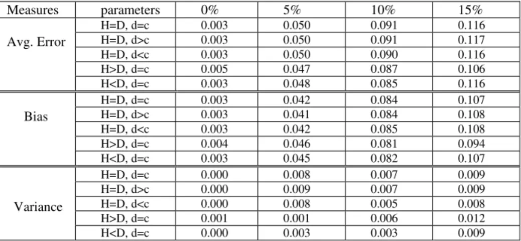
will be as-signed the class label “+1”. To simulate noisy instances, we randomly pick up 0.0%, 0.25%, 5%, 7.5% instances from each class and then assign them the opposite class label. In the following experiments, we will do bias-variance decomposition on these four datasets to investigate whether RMCLP is a stable and strong classifier.

Table 1 reports the 10-folder cross validation of bias variance results on the syn-thetic datasets. The first column lists three measurements, average error, bias error and variance error respectively. The second column shows the different parameters of RMCLP. The 3th to 6th column lists the experiment results under different training samples. In this experiments, we will do the following observations: (1) by using different parameters of (H,D,d,c), we examine whether RMCLP varies significantly different on different parameters; (2) by comparing the bias and variance errors, we get a conclusion where the error mainly comes from, and thus we can define RMLCP as a strong or weak classifier, a stable or unstable classifier. However, we don’t report the noise error N(x) here because noises error is independent of classifiers but only related to the nature of dataset. Additionally, we give approximate values to bias error by subtract variance error from the average error. This approximation is reasonable because it won’t change their orders when compared. All of the numeric results are listed in Table 1.

From the results of average errors, we can observe that the error rates have slight changes when the parameters keep changing. On the 0% noise dataset, only when H>D, the error goes up from 0.003 to 0.005. On the other three datasets, these similar tendencies have been observed. Thus we can say that RMCLP is slightly impacted by different parameters.

From the variance error, we can observe that compared to the average errors and bias errors, the variance errors take a low percentage of the whole error. For example, on 0% noise dataset, most of the variance errors stay 0, that is to say, no changes have been observed. On the other three datasets, the variance error are almost 10-1 lower than the bias error. Thus it is safe to say that RMCLP is a stable classifier, and bag-ging will help little on RMCLP model.

From the bias error, we can see that on the four datasets, bias errors take part of most of the average errors. For example, on the 10% noise dataset, when H=D, d=c, the average error is 0.091, while the bias errors is 0.084, which takes up 92.3% of the whole error. Thus it is also safe to say that RMCLP is not a strong classifier, and boosting can be used to enhance RMCLP into a strong classifier.

Table 1. Results ofBias variance analysis Measures parameters 0% 5% 10% 15% H=D, d=c 0.003 0.050 0.091 0.116 H=D, d>c 0.003 0.050 0.091 0.117 H=D, d<c 0.003 0.050 0.090 0.116 H>D, d=c 0.005 0.047 0.087 0.106 Avg. Error H<D, d=c 0.003 0.048 0.085 0.116 H=D, d=c 0.003 0.042 0.084 0.107 H=D, d>c 0.003 0.041 0.084 0.108 H=D, d<c 0.003 0.042 0.085 0.108 H>D, d=c 0.004 0.046 0.081 0.094 Bias H<D, d=c 0.003 0.045 0.082 0.107 H=D, d=c 0.000 0.008 0.007 0.009 H=D, d>c 0.000 0.009 0.007 0.009 H=D, d<c 0.000 0.008 0.005 0.008 H>D, d=c 0.001 0.001 0.006 0.012 Variance H<D, d=c 0.000 0.003 0.003 0.009

6 Conclusions

In this paper, we applied bias-variance decomposition to RMCLP learning algorithms for the purposes of gaining a thorough understanding of RMCLP’s stability and weak-ness for classification. Our theoretical and empirical studies have concluded that : (1) The parameter setting (H,D,d,c) has very limited impact on the performance of the RMCLP models; (2) The variance of the RMCLP models accounts for only a small part of the total testing error, which indicates that RMCLP is a stable classifier; (3) The testing error of RMCLP mostly comes from its bias, which suggests that RMCLP doesn’t belong to the strong learner category; (4) Bagging has a limited effect on RMCLP as it is a stable learner; (5) By using boosting method (especially adaboost-ing), we can transform RMCLP into a strong classifier. In the future, we will use this bias variance decomposition to test RMCLP model on UCI benchmark datasets to further validate our conclusions.

References

1. Bennett, K.P., Parrado-Hernandez, E.: The Interplay of Optimization and Machine Learn-ing Research. Journal of Machine LearnLearn-ing Research 7, 1265–1281 (2006)

2. Shi, Y., Wise, M., Luo, M., Lin, Y.: Data mining in credit card portfolio management: a multiple criteria decision making approach. Multiple Criteria Decision Making in the New Millennium, 427–436 (2001)

3. Shi, Y., Tian, Y., Chen, X., Zhang, P.: A Regularized Multiple Criteria Linear Program for Classification. In: ICDM Workshops 2007, pp. 253–258 (2007)

4. Kong, E.B., Dietterich, T.G.: Error-correcting output coding corrects bias and variance. In: Proc. of the 12th ICML Conference (1996)

5. Domingos, P.: A Unified Bias-Variance Decomposition and its Applications. In: Proc. of thseventeeth Interntional Conference on Machine Learning, Stanford, CA, pp. 231–238. Morgan Kaufmann, San Francisco (2000)

6. Domingos, P.: A Unifed Bias-Variance Decomposition for Zero-One and Squared Loss. In: Proc. of the Seventeenth National Conference on Artificial Intelligence, Austin, TX. AAAI Press, Menlo Park (2000)

7. Valentini, G., Dietterich, T.G.: Bias-Variance Analysis of Support Vector Machines for the Development of SVM-Based Ensemble Methods. Journal of Machine Learning Re-search 5, 725–775 (2004)

8. Breiman, L.: Bagging predictors. Journal of Machine Learning 24, 123–140 (1996) 9. Freund, Y., Schapire, R.E.: A decision-theoretic generalization of on-line learning and an

application to boosting. Journal of Computer and System Sciences 55(1), 119–139 (1997) 10. Polikar, R.: Ensemble Based Systems in Decision Making. IEEE Circuits and Systems

Magazine 6(3), 21–45 (2006)

11. Peng, Y., Kou, G., Chen, Z., Shi, Y.: Cross-Validation and Ensemble Analyses on Multi-ple-Criteria Linear Programming Classification for Credit Cardholder Behavior. In: Inter-national Conference on Computational Science, pp. 931–939 (2004)

Appendix

In this appendix we give the deduction of the original bias variance decomposition in regression problems with squared-lose function.

Assume the genuine function we want to approximate is f = f x( ). There is a train-ing sample {( , )} 1

N i i i

D= x t ₌ , where xi∈X , for instance d

X =\ , d∈N and

i

t ∈T with T=\. Besides, D contains a noise level ε with expectation of 0, that is to say, t= +f εand ( )E ε =0. A learning function g=g(w,x) is used to approximate the genuine function f , where w is the parameters of g and x is the training sample. To a specific xi, g gives a corresponding value yi=g(w,xi). Thus, the mean squared loss of

g on the whole training dataset D is

1 ( , ) 1 ₁( )2 | | N i i i x D MSE L g x dx t y D ∈ N = =

∫

=

∑

− .

To investigate whether g is a good regression model on D, we calculate the expecta-tion of the mean squared loss by

2 2 1 1 1 1 { } { N (_{i i}) } { N (_{i i}) } i i E MSE E t y E t y N = N = =

∑

− =

∑

− . (13)

To get {E MSE}, we calculate 2

(i i) E⎡_⎣t −y ⎤_⎦ as follows: 2 2 (i i) (i i i i) E_⎣⎡t −y _⎦⎤=E_⎣⎡t − + −f f y ⎤_⎦ (14) 2 2 (i i) ( i i) 2(i i)( i i) E⎡t f f y t f f y ⎤ = _⎣ − + − + − − _⎦

[

]

2 2 (i i) ( i i) 2 (i i)( i i) E t f E f y E t f f y = − + − + − −

(

)

2 2 2 ( )_i ( _{i i}) 2 (_{i i}) (_{i i}) ( _i ) ( _{i i}) E ε E f y ⎡ E t f E t y E f E f y ⎤ = + − + _⎣ − − + _⎦

(

)

2 2 2 ( i ) ( i i) 2 (i i) (i i) ( i ) ( i i) E ε E f y ⎡ E t f E t y E f E f y ⎤ = + − + _⎣ − − + _⎦

As we discussed above, t= +f ε and ( )E ε =0, thus we have the following two equations:

2 2 (i i) ( i i i) ( i ) E t f =E f +ε f =E f , (15) (i i) ( i i i i) ( i i) E t y =E f y +εy =E f y . (16) Meanwhile 2 2 ( i i) ( i ( )i ( )i i) E f −y =E f −E y +E y −y (17)

(

)

2

(

)

2

(

)

( ) ( ) 2 ( ( ))( ( ) ) i i i i i i i i E f E y E E y y E f E y E y y = − + − + − −

(

)

2

(

)

2

(

2 2

)

( ) ( ) 2 ( ) ( ) ( ) ( ) ( ) i i i i i i i i i i E f E y E E y y E f E y E f y E y E y = − + − + − − + =E f

(

_i−E f( )_i

)

2+E E f

(

( )_i −y_i

)

2

Consequently, by combining (14), (15), (16) and (17), we can get the result of (13) as follows: 2 { } (i i) E MSE ∝E⎡_⎣ t −y ⎤_⎦ 2 2

(

_i

)

(

_{i i}

)

E

ε

E f

y

=

+

−

=

(

)

(

)

2 2 2 2

(

_i

)

_i

(

_i

)

(

_i

)

_i

noise Bias Variance

E

ε

+

E f

−

E y

+

E E y

−

y

We can see that under this decomposition, the average error of a learner g is com-posed of its noise, bias and variance errors. Noise error is the inherent characteristics of the training sample that we can do nothing to improve. Bias error is the error be-tween the target function f and the average output of learning algorithm g. Variance error is the error between the individual output of g and the average output of g.