SpArch: Efficient Architecture for Sparse Matrix Multiplication

(1)

SpArch: Efficient Architecture for Sparse Matrix Multiplication

Zhekai Zhang∗, Hanrui Wang∗, Song Han

EECS

Massachusetts Institute of Technology Cambridge, MA, US

{zhangzk, hanrui, songhan}@mit.edu

William J. Dally

Electrical Engineering Stanford University / NVIDIA

Stanford, CA, US [email protected]

Abstract—Generalized Sparse Matrix-Matrix Multiplication (SpGEMM) is a ubiquitous task in various engineering and scientific applications. However, inner product based SpGEMM introduces redundant input fetches for mismatched nonzero operands, while outer product based approach [1] suffers from poor output locality due to numerous partial product matrices. Inefficiency in the reuse of either inputs or outputs data leads to extensive and expensive DRAM access.

To address this problem, this paper proposes an efficient sparse matrix multiplication accelerator architecture, SpArch, which jointly optimizes the data locality for both input and output matrices. We first design a highly parallelized

streaming-based mergerto pipeline the multiply and merge stage of partial

matrices so that partial matrices are merged on chip

imme-diately after produced. We then propose a condensed matrix

representationthat reduces the number of partial matrices by

three orders of magnitude and thus reduces DRAM access by

5.4×. We further develop aHuffman tree schedulerto improve

the scalability of the merger for larger sparse matrices, which

reduces the DRAM access by another 1.8×. We also resolve the

increased input matrix read induced by the new representation

using a row prefetcher with near-optimal buffer replacement

policy, further reducing the DRAM access by 1.5×. Evaluated

on 20 benchmarks, SpArch reduces the total DRAM access

by 2.8× over previous state-of-the-art. On average, SpArch

achieves 4×, 19×, 18×, 17×, 1285×speedup and 6×, 164×,

435×, 307×, 62× energy savings over OuterSPACE, MKL,

cuSPARSE, CUSP, and ARM Armadillo, respectively. Keywords-Sparse Matrix Multiplication; Domain-Specific Architecture; Specialized Accelerators; Huffman-Tree; Data Reuse

I. INTRODUCTION

Generalized sparse matrix-matrix multiplication (SpG-EMM) is the key computing kernel for many algorithms such as compressed deep neural networks [2], [3], [4], [5], triangle counting [6], Markov clustering [7], searching algorithms [8], [9], and matching algorithms [10]. It is also ubiquitous in scientific and engineering applications such as grammar parsing [11], chemical molecule dynamics [12], color intersection search [13], linear solver [14] and many other applications [15], [16], [17], [18], [19].

However, the performance of SpGEMM is memory bounded on the traditional general-purpose computing plat-forms such as CPUs and GPUs, because of the irregular

∗_{Equal Contributions.} First Matrix A

=

Second Matrix B a1 aN-1 b1 bN-1 CN-1 Partial Matrices Ci Resultant Matrix C C1 C0

Multiply Stage Merge Stage Final Results

0.6 1.3

2.2 1.1

Partial Matrix A Partial Matrix B

0.1 0.5 0.2 1.2

+

0.1 1.1 0.2 1.3 2.2 1.1 1.2

=

Sorted Merged (1, 0.1)(3, 1.1)(4, 0.2)(5, 1.3)(10, 2.2)(12, 1.1)(13, 0.1) (1, 0.1)(3, 0.5)(3, 0.6)(4, 0.2)(5, 1.3)(10, 2.2)(12, 1.1)(13, 0.1) 0 1 2 3 4 5 6 7 Comparator Array (1, 0.1) (3, 0.5) (4, 0.2)(13, 1.2) (3, 0.6) (5, 1.3) (10, 2.2) (12, 1.1) ≥ ≥ < ≥ ≥ ≥ ≥ ≥ ≥ ≥ ≥ ≥ 0 1 2 3 1 2 3 4 2 3 4 5 3 4 5 6,7 < < < < < < < < ≥ ≥ ≥ ≥ 3 4 5 6 4 5 6 7 4 5 6 7 A0 B0 (1, 0.1) (3, 0.5) (4, 0.2) Pa rt ia l Ma tri x A (3, 0.6) (5, 1.3)(10, 2.2) (12, 1.1) (15, 4.4)(29, 3.9) (35, -1.1)(40, 9.2) (44, 7.1)(52, -1.0) (55, 0.2) (61, 9.9) Chunk A0 (13, 1.2) (19, 5.1)(22, -3.1) (35, 1.2)(37, 9.2) (42, 1.1)(47, 9.9) (48, 0.3)(58, -10.8) Pa rt ia l Ma tri x B Chunk A1 Chunk A2

Chunk B0 Chunk B1 Chunk B2

< < < ≥ ≥ < ≥ ≥ ≥ 0 1 2 1 2 3 2 3 4 A0 (13, 1.2) A1 (37, 9.2) A2 (58, -10.8) B0(12, 1.1) B1 (40, 9.2) B2 (61, 9.9) Decide chunk Pairs for low level comparator arrays B1 B1 A2 B1 A2 B2 0 1 2 3 4 Top level comparator array compares last element

in each chunk

Low level comparator arrays compare chunk pairs

in parallel A0 A1 A0 B0 Zoom In (1, 0.1) (3, 0.5) (4, 0.2)(13, 1.2) (3, 0.6) (5, 1.3) (10, 2.2) (12, 1.1) ≥ ≥ < ≥ ≥ ≥ ≥ ≥ ≥ ≥ ≥ ≥ 0 1 2 3 1 2 3 4 2 3 4 5 3 4 5 6,7 < < < < < < < < ≥ ≥ ≥ ≥ 3 4 5 6 4 5 6 7 4 5 6 7 R0-0 R0 R0-1 R0-2 R0-3 R0-4 R0-5 R0-6 R1-0 R1 R1-1 R1-2 R1-3 R2-0 R2 R2-1 R2-2 R2-3 R2-4 R2-5 R2-6 R2-7 R2-8 R2-9 R3-0 R3 R3-1 R3-2 R4-0 R4 R4-1 R4-2 R4-3 R4-4 R4-5 Replace R0 then Replace R1 R1-0 R1-1 R1-2 R1-3 C1 R1-0 R1-1 R1-2 R1-3 R0-0 R0-1 R0-2 R0-3 R0-4 R0-5 R0-6 C0 R2-8 R2-9 R1-2 R1-3 R2-1 R2-2 R2-3 R2-4 R2-5 R2-6 R2-7 R2-0 C2 R2-8 R2-9 R3-0 R3-1 R2-1 R2-2 R2-3 R2-4 R2-5 R2-6 R2-7 R3-2 C3 Replace R1 then Replace R2 R2-8 R2-9 R2-0 R3-1 R2-1 R2-2 R2-3 R2-4 R2-5 R2-6 R2-7 R3-2 C2 Replace R3 R2-8 R2-9 R1-0 R3-1 R1-1 R1-2 R1-3 R2-4 R2-5 R2-6 R2-7 R3-2 C1 Replace R2 R4-4 R4-5 R1-0 R3-1 R1-1 R1-2 R1-3 R4-0 R4-1 R4-2 R4-3 R3-2 C4 Replace R2 R4-4 R4-5 R1-0 R3-1 R1-1 R1-2 R1-3 R4-0 R4-1 R4-2 R4-3 R3-2 C1 Replace R4 R4-4 R4-5 R1-0 R3-1 R1-1 R1-2 R1-3 R3-0 R4-1 R4-2 R4-3 R3-2 C3 Replace R3 then Replace R4 R0-6 R4-5 R1-0 R0-1 R1-1 R1-2 R1-3 R0-0 R0-3 R0-4 R0-5 R0-2 C0 R0-6 R4-5 R1-0 R0-1 R1-1 R1-2 R1-3 R0-0 R0-3 R0-4 R0-5 R0-2 C1 R0-6 R4-5 R1-0 R0-1 R1-1 R1-2 R1-3 R0-0 R0-3 R0-4 R0-5 R0-2 C0 C1 C0 C2 C3 C2 C1 C4 C1 C3 C0 C1 C0 C4 C4 C1 C0 D ist an ce : 7 D ist an ce

: 3 Step0 Step1 Step2 Step3 Step4 Step5 Step6 Step7 Step8 Step9 Step10 Step11

H BM MatB Row Prefetcher Mu ltip lie r Arra y MatA Column Fetcher Distance List Builder Look-Ahead FIFO Required

Row DistanceRow

MatA Element MatB Row Merger Merger New PMat Merger FIFO Partial Mat Fetcher Partial Mat Addr

Partial Mat Writer Old PMat zero_count 0 01 2 2 2 3 3 iter1: if zero_count[0] == 1 shift left by 1 3 1 0 0 2 3 0 4 0 1 0 0 2 3 4 0 0 zero_count 0 0 12 2 2 2 iter2: if zero_count[1] == 1 shift left by 2 1 0 0 2 3 4 0 0 1 2 3 4 0 0 0 0 Ma tri x C on de nsi ng Round 0 Round 1 Round 2 Lo ad Se qu en ce

Produces 16 partial matrices Produces 12 partial matrices

Matrix Condensing stored in CSR loaded by condensed column 1st 4th 2nd 3rd Pipelined Multiply

and Merge Matrix Condensing Huffman Tree Scheduler Row Prefetcher

5.7x slowdown 5.7x more DRAM access

8.8x speedup 5.4x less DRAM access

Overall 4.2x speedup 2.8x less DRAM access 1.5x speedup

1.8x less DRAM access

Better Output Reuse Better Input Reuse

Merger (Comparator Array)

26 31 28 42 13 15 14 16

22 24 11 12

Merger (Comparator Array) DRAM

A B C D

Multiplier Array Merger (Comparator Array)

24 26 22 28 11 13 12 14

A B C D

26 31 28 42

Merger (Comparator Array) 22 24

15 21 16 17

13 14

11 12

26 31 28 42 21 23 17 19

22 24 15 16

13 14

Merger (Comparator Array) DRAM 11, 12 Multiplier Array A: (24)(26)(31)(52)(54)(56)(57)(58)(73)(75) B: (22)(28)(42)(44)(46)(47)(48) C: (11)(13)(15)(21)(23)(25)(41)(43)(45) D: (12)(14)(16)(17)(18)(32)(34)(36)(37)(38)(72) R8 A 15

2-Way with Sequential Scheduler

total weight of all nodes: 365 A 15 B 15 C 13 D 12 E 9 F 7 G 3 H 2 I 2 J 2 K 2 L 2

weight∝memory access (a)

2-Way with Huffman Tree Scheduler

C 28 B 15 13 A 15 E 9 17 K 2 L 2 4 I 2 J 2 4 8 32 F 7 5 12 G 3 H 2 12 D 24 52 84

R: Round total weight of all nodes reduces to: 354

R0 R2 R6 R5 R4 R1 R7 B 15 C 13 D 12 E 9 F 7 G 3 H 2 I 2 J 2 K 2 L 2

weight∝memory access (b)

J 2 K 2 L 2 6 C 13 G 3 H 2 I 2 A 15 B 15 D 12 E 9 F 7 13 41 84 R0 R1 R2 R3 A 1515B 13 C 12D E 9F 7G 3H 22I J 2K 22L

total weight of all nodes reduces to: 228 weight∝memory access R: Round (c) A 4 D L K 2 7 C 2 I 9 4 13 16 17 33 5 J 2 B 2 G 15 16 15 H 2 F 3 20 31 51 84 E 12 Vanilla Inner Product Based

=

PoorInput Reuse Good Output Reuse

A B C Vanilla Outer Product Based

=

Good Input Reuse

{

Poor Output Reuse

me rge ma ny part ial ma trice_s D E H G F Proposed Outer Product Based

=

Good Input Reuse Good Output Reuse

❸ Huffman Tree Scheduler

❹ Row Prefetcher

❶ Pipelined Multiply and Merge

❷ Matrix Condensing Less Partial Matrices

{

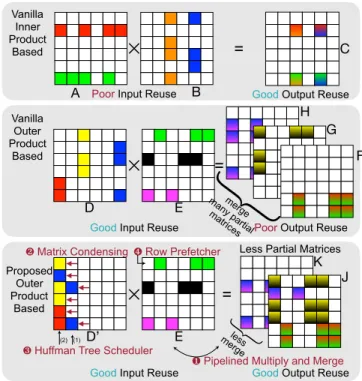
less me rge (1) (2) J K E D’

Figure 1. Proposed outer product based SpGEMM architecture jointly optimizes input and output data reuse. It achieves good output reuse with pipelined multiply and merge, matrix condensing, Huffman tree scheduler, good input reuse with row prefetcher.

memory access pattern and poor locality caused by low-density matrices [20], [21], [22]. For instance, the low-density of Twitter’s [23] adjacency matrix is as low as 0.000214%. As Moore’s Law [24] is slowing down, domain-specific archi-tecture [25] becomes promising to improve performance and energy efficiency. OuterSPACE [1] proposedouter product

based SpGEMM, which has perfect input reuse compared

to inner product based method. However, outer product

has poor output reuse because it produces a considerable amount of partial matrices (F,G,H in Figure 1). Those

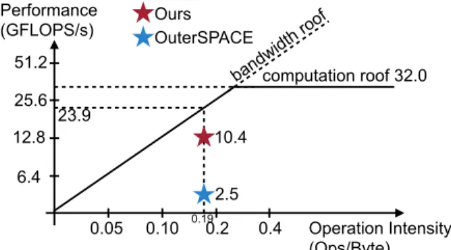
partial matrices need to be stored to DRAM before merg-ing, which incurs extensive DRAM access and cancels the benefits of good input reuse. As a result, the performance of OuterSPACE is only 10.4% of the theoretical peak.

(2)

Pipelined Multiply

and Merge Matrix Condensing Huffman Tree Scheduler Row Prefetcher

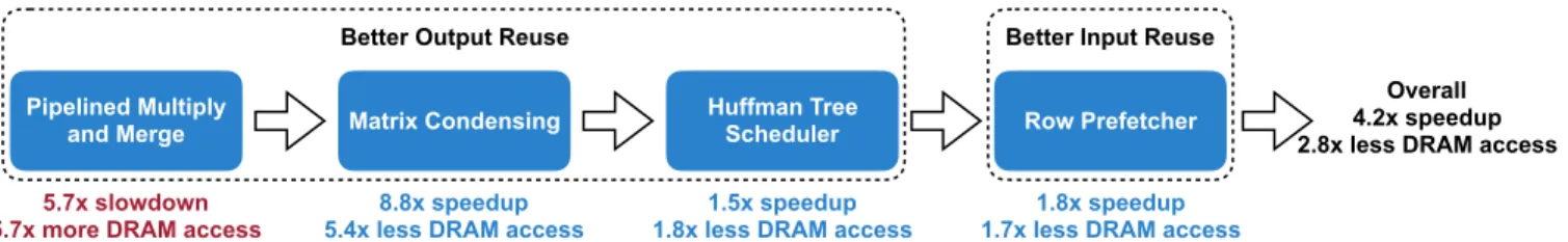
Figure 2. Four innovations in SpArch. The first slowdown is because of the excessive memory access of partially merged results when the number of partial matrices is much larger than merge tree parallelism. But it enables the next three optimizations. We save DRAM bandwidth, achieve higher memory utilization and speedup.

In this paper, we propose SpArch1_{, a domain-specific}

accelerator to jointly optimize input and output data reuse. We obtain input reuse by outer product, and output reuse by on-chip partial matrix merging.

To achieve this, we design a highly parallelized merger to pipeline the two computing stages, multiply and merge. The multiply stage produces partial matrices, and themerge

stage merges partial matrices into final results. For large matrices, however, the number of partial matrices exceeds the merger’s parallelism. Merging only a part of partial matrices at a time with multiple rounds leads to an increased amount of memory access for the partially merged results, which neutralizes the performance gain of pipelined multiple and merge, making DRAM access even larger (see the first step of Figure 2). However, it is a prerequisite for the next three optimizations. Therefore, we propose a condensed matrix representation for the first input matrix, where all non-zero elements are pushed to the left, forming much denser columns. As shown in Figure 1, we condense the first input matrixDto condensedD0. The condensed matrix D0 is loaded by condensed column. Implementation-wise,

this is equivalent to storing the matrix in CSR format and fetching the elements with the same index for all rows. The second input matrixEis stored in CSR format. The original

left matrix_D has three columns and produces three partial matrices. After condensing, _D0 only has two columns and only two partial matrices. In real-world benchmarks, we save the number of partial matrices by three orders of magnitude. Unfortunately, the condensed representation can still pro-duce a larger amount of partial matrices than the merger’s parallelism. The merge order impacts the amount of DRAM access: partial matrices mergedearlyhave to be load/stored to DRAM for every future merges. Therefore, we should merge matrices with less non-zeros first. We design a

Huffman tree scheduler to decide the near-optimal merge

order. We represent each column of a sparse matrix as a leaf node. The weight of the node is the number of non-zeros in that column. For very sparse matrices, the number of non-zeros after merge is approximately the sum of the number of non-zeros before merge. Therefore, the weight of

1_{SpArch is the homophone of word}_spark_{, meaning striking together two} hard surfaces such as stone or metal, which we consider as analogous to

matrix-condensing, a critical technique in our architecture.

a parent node is the sum of the children’s weights, exactly following the convention of a Huffman tree. A Huffman tree minimizes the sum of all nodes’ weights. We apply

it to minimize the total DRAM traffic. Scheduled by

a Huffman tree, we merge matrices with fewer non-zeros first and larger ones later (example in Figure 8). The three techniques discussed above save output DRAM access on 20 benchmarks by1/5.7×5.4×1.8 = 1.7× compared to OuterSPACE (Figure 2).

However, in matrix condensing step, we ruin the perfect reuse of the second matrix (Ein Figure 1) because now one

condensed column ofD0 need all the three (green, black and

pink) rows ofE. In contrast, one column ofDonly needs one

row ofE. Therefore, we propose arow prefetcherto prefetch

rows of the second matrixEand store to a row buffer. The

buffer replacement policy is near-optimal because we look at the sequence of the rows we need ahead of time while streaming in the first matrix, and thus we can replace the line with farthest next use. The row buffer can achieve a 62% hit rate, thus reducing DRAM access of the second matrix by 2.6×, largely recovering the input reuse. With the four techniques together, we reduce DRAM access by 2.8×over OuterSPACE.

In summary, SpArch jointly optimizes input and output reuse of SpGEMM and makes five contributions:

• Pipeline the multiply stage and the merge stage with a

comparator array-based highly parallelizedmerger.

• Usematrix-condensingto condense the first input ma-trix, reducing the number of partial matrices by three orders of magnitude.

• AHuffman tree scheduler that provides a near-optimal merge order of partial matrices and reduces the DRAM traffic.

• A row prefetcher that achieves near-optimal buffer

replacement policy for the second input matrix and resolves the increased DRAM read induced by matrix-condensing.

• We evaluate SpArch on real-world datasets from SuiteSparse [26], SNAP [27] and rMAT [28], achieving 4×, 19×, 18×, 17×, 1285×speedup, and 6×, 164×, 435×, 307×, 62× energy saving over OuterSPACE, MKL, cuSPARSE, CUSP and ARM Armadillo.

(3)

First Matrix A

=

3 zero_count 0 012 2 2 3 iter1: if zero_count[0] == 1 shift left by 1 1 0 0 2 3 0 4 0 1 0 0 2 3 4 0 0 3 zero_count 0 0 12 2 2 2 iter2: if zero_count[1] == 1 shift left by 2 1 0 0 2 3 4 0 0 1 2 3 4 0 0 0 0 Ma tri x C on de nsi ng Round 0 Round 1 Round 2 Lo ad Se qu en ce

Produces 16 partial matrices Produces 12 partial matrices Matrix Condensing stored in CSR, loaded by condensed column 1st 4th 2nd 3rd Pipelined Multiply

and Merge Matrix Condensing

Huffman Tree

Scheduler Row Prefetcher

26 31 28 42 13 15 14 16

22 24 11 12

DRAM

A B C D

Multiplier Array

24 26 22 28 11 13 12 14

DRAM

A B C D

26 31 28 42

15 21 16 17

13 14

11 12

DRAM

26 31 28 42 21 23 17 19

22 24 15 16

13 14

DRAM 11,12 Multiplier Array A: (24)(26)(31)(52)(54)(56)(57)(58)(73)(75) B: (22)(28)(42)(44)(46)(47)(48) C: (11)(13)(15)(21)(23)(25)(41)(43)(45) D: (12)(14)(16)(17)(18)(32)(34)(36)(37)(38)(72) Vanilla Inner Product Based

=

Good Input Reuse

{

Poor Output Reuse

=

❹ Row Prefetcher

{

less me rge (1) (2) J K E D’ R8 A 15 2-Way with Sequential Scheduler

Total weight of all nodes: 365 A 15 B 15 C 13 D 12 E 9 F 7 G 3 H 2 I 2 J 2 K 2 L 2

weight

∝

memory access (a)

C 28 B 15 13 A 15 E 9 17 K 2 L 2 4 I 2 J 2 4 8 32 F 7 5 12 G 3 H 2 12 D 24 52 84

R: Round Total weight of all nodes reduces to: 354

R0 R2 R6 R5 R4 R1 R7 B 15 C 13 D 12 E 9 F 7 G 3 H 2 I 2 J 2 K 2 L 2 (b)

J 2 K 2 L 2 6 C 13 G 3 H 2 I 2 A 15 B 15 D 12 E 9 F 7 13 41 84 R0 R1 R2 R3 A 1515B 13 C 12D E 9F 7G 3H 22I J 2K 22L

Total weight of all nodes reduces to: 228 (c) A 4 D L K 2 7 C 2 I 9 4 13 16 17 33 5 J 2 B 2 G 15 16 15 H 2 F 3 20 31 51 84 E 12 0.6 1.3 2.2 1.1 Partial Matrix B Partial Matrix A 0.1 0.5 0.2 1.2

+

0.1 1.1 0.2 1.3 2.2 1.1 1.2

=

Merged (1, 0.1)(3, 1.1)(4, 0.2)(5, 1.3)(10, 2.2)(12, 1.1)(13, 0.1) Sorted (1, 0.1)(3, 0.5)(3, 0.6)(4, 0.2)(5, 1.3)(10, 2.2)(12, 1.1)(13, 0.1) 0 1 2 3 4 5 6 7 Comparator Array (1, 0.1) (3, 0.5)(4, 0.2)(13, 1.2) (3, 0.6) (5, 1.3) (10, 2.2) (12, 1.1) ≥ ≥ < ≥ ≥ ≥ ≥ ≥ ≥ ≥ ≥ ≥ 0 1 2 3 1 2 3 4 2 3 4 5 3 4 5 6,7 < < < < < < < < ≥ ≥ ≥ ≥ 3 4 5 6 4 5 6 7 4 5 6 7 A0 B0 < < < ≥ ≥ < ≥ ≥ ≥ 0 1 2 1 2 3 2 3 4 A0 (13, 1.2) A1 (37, 9.2) A2 (58, -10.8) B0 (12, 1.1) B1 (40, 9.2) B2 (61, 9.9) _Deci de ch un k Pa irs fo r lo w le ve l co mp ara to r arra ys B1 B1 A2 B1 A2 B2 0 1 2 3 4 Top level comparator array compares last element

in each chunk

in parallel A0 A1 A0 B0 Zoom In (1, 0.1) (3, 0.5)(4, 0.2)(13, 1.2) (3, 0.6) (5, 1.3) (10, 2.2) (12, 1.1) ≥ ≥ < ≥ ≥ ≥ ≥ ≥ ≥ ≥ ≥ ≥ 0 1 2 3 1 2 3 4 2 3 4 5 3 4 5 6,7 < < < < < < < < ≥ ≥ ≥ ≥ 3 4 5 6 4 5 6 7 4 5 6 7 (1,0.1)(3,0.5)(4,0.2) Chunk A0 (13,1.2) (19,5.1)(22,-3.1)(35,1.2)(37,9.2) Chunk A1 (42,1.1)(47,9.9)(48,0.3)(58,-10.8) Chunk A2 Partial Matrix A (3,0.6)(5,1.3)(10,2.2)(12,1.1)

Chunk B0 (15,4.4)(29,3.9)(35,-1.1)(40,9.2)Chunk B1 (44,7.1)(52,-1.0)(55,0.2)(61,9.9)Chunk B2 Partial Matrix B R0-0 R0 R0-1 R0-2 R0-3 R0-4 R0-5 R0-6 R1-0 R1 R1-1 R1-2 R1-3 R2-0 R2 R2-1 R2-2 R2-3 R2-4 R2-5 R2-6 R2-7 R2-8 R2-9 R3-0 R3 R3-1 R3-2 R4-0 R4 R4-1 R4-2 R4-3 R4-4 R4-5 Replace R0 then Replace R1 R1-0 R1-1 R1-2 R1-3 C1 R1-0 R1-1 R1-2 R1-3 R0-0 R0-1 R0-2 R0-3 R0-4 R0-5 R0-6 C0 R2-8 R2-9 R1-2 R1-3 R2-1 R2-2 R2-3 R2-4 R2-5 R2-6 R2-7 R2-0 C2 R2-8 R2-9 R3-0 R3-1 R2-1 R2-2 R2-3 R2-4 R2-5 R2-6 R2-7 R3-2 C3 Replace R1 then Replace R2 R2-8 R2-9 R2-0 R3-1 R2-1 R2-2 R2-3 R2-4 R2-5 R2-6 R2-7 R3-2 C2 Replace R3 R2-8 R2-9 R1-0 R3-1 R1-1 R1-2 R1-3 R2-4 R2-5 R2-6 R2-7 R3-2 C1 Replace R2 R4-4 R4-5 R1-0 R3-1 R1-1 R1-2 R1-3 R4-0 R4-1 R4-2 R4-3 R3-2 C4 Replace R2 R4-4 R4-5 R1-0 R3-1 R1-1 R1-2 R1-3 R4-0 R4-1 R4-2 R4-3 R3-2 C1 Replace R4 R4-4 R4-5 R1-0 R3-1 R1-1 R1-2 R1-3 R3-0 R4-1 R4-2 R4-3 R3-2 C3 Replace R3 then Replace R4 R0-6 R4-5 R1-0 R0-1 R1-1 R1-2 R1-3 R0-0 R0-3 R0-4 R0-5 R0-2 C0 R0-6 R4-5 R1-0 R0-1 R1-1 R1-2 R1-3 R0-0 R0-3 R0-4 R0-5 R0-2 C1 R0-6 R4-5 R1-0 R0-1 R1-1 R1-2 R1-3 R0-0 R0-3 R0-4 R0-5 R0-2 C0 C1 C0 C2 C3 C2 C1 C4 C1 C3 C0 C1 C0 C4 C4 C1 C0 D ist an ce : 7 D ist an ce

H BM MatB Row Prefetcher Mu ltip lie r Arra y MatA Column Fetcher Distance List Builder Look-Ahead FIFO Required Row Row Distance MatA Element MatB Row Merger Merger New PMat Merger FIFO Partial Mat Fetcher Partial Mat Addr

Partial Mat Writer Old

PMat

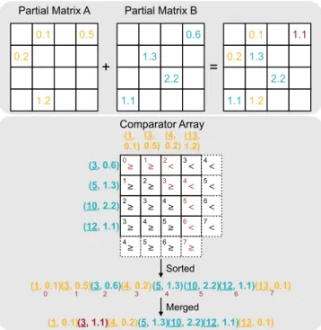
Figure 3. Comparator Array Based Merger. Each diagonal group outputs the data on the boundary of ”≥” and ”<” to form a sorted array. The adder and zero eliminator will further merge the duplicated elements.

II. PROPOSEDARCHITECTURE

A. Comparator Array based Merger

Previous state-of-the-art SpGEMM accelerator [1] pro-cesses multiply and merge stages separately, which need to store all partial matrices in DRAM. A better way is to pipeline the multiply and merge stages and perform an on-chip merge. The partial matrix is represented in COO format with [row index, column index, value]. It is sorted by row index then column index. The merger combines multiple sorted arrays into a new sorted array. A simple merger puts each array into a FIFO and selects the smallest elements from the top of all FIFOs. This method suffers from low parallelism and thus cannot fully utilize the DRAM bandwidth. Therefore, we design a parallel merge unit.

1) Parallel Merge Unit: A na¨ıve merger walks two

pointers over two arrays and compares the corresponding elements. The pointer with the smaller element will move forward. This only outputs one element per cycle. In order to increase the parallelism, we replace the pointer by a sliding window of size N, all elements in the window A will be compared to all elements in window B by an array of comparators. After the comparison, we move one of the window forward by N, improving the throughput by N

times.

A comparator array is the core of our merge unit. As in Figure 3, the merger contains 4×4 comparators. The two input matrices are stored in the format of [coordinate, value]. We use the comparator array to compare coordinates of all

First Matrix A = = Second Matrix B a1 aN-1 b1 bN-1 CN-1 Partial Matrices Ci Resultant Matrix C C1 C0

3 zero_count 0 012 2 23 iter1: if zero_count[0] == 1 shift left by 1 1 0 0 2 3 0 4 0 1 0 0 2 3 4 0 0 3 zero_count 0 0 12 2 2 2 iter2: if zero_count[1] == 1 shift left by 2 1 0 0 2 3 4 0 0 1 2 3 4 0 0 0 0 Ma tri x C on de nsi ng Round 0 Round 1 Round 2 Lo ad Se qu en ce

Matrix Condensing stored in CSR, loaded by condensed column 1st 4th 2nd 3rd Pipelined Multiply

and Merge Matrix Condensing Huffman Tree Scheduler Row Prefetcher

5.7x slowdown

5.7x more DRAM access 5.4x less DRAM access8.8x speedup

Overall 4.2x speedup 2.8x less DRAM access

1.5x speedup

1.8x less DRAM access 1.7x less DRAM access1.8x speedup

26 31 28 42 13 15 14 16

2224 11 12

A B C D

24 26 22 28 11 13 12 14

A B C D

26 31 28 42

2224

15 21 16 17

1314

11 12

A B C D

26 31 28 42 21 23 17 19

2224 1516

1314

Merger (Comparator Array) DRAM A B C D 11,12 Multiplier Array Multiplier Array Multiplier Array A: (24)(26)(31)(52)(54)(56)(57)(58)(73)(75) B: (22)(28)(42)(44)(46)(47)(48) C: (11)(13)(15)(21)(23)(25)(41)(43)(45) D: (12)(14)(16)(17)(18)(32)(34)(36)(37)(38)(72) Vanilla Inner Product Based =

A B C Vanilla Outer Product Based =

Good Input Reuse

{

Poor Output Reuse

me rge ma ny part ial ma trice_s D E H G F Proposed Outer Product Based =

Good Input Reuse Good Output Reuse ❸ Huffman Tree Scheduler

❹ Row Prefetcher

{

less me rge (1) (2) J K E D’ R8 A 15

Total weight of all nodes: 365

A 15 B 15 C 13 D 12 E 9 F 7 G 3 H 2 I 2 J 2 K 2 L 2

weight∝memory access

(a)

C 28 B 15 13 A 15 E 9 17 K 2 L 2 4 I 2 J 2 4 8 32 F 7 5 12 G 3 H 2 12 D 24 52 84

J 2 K 2 L 2 6 C 13 G 3 H 2 I 2 A 15 B 15 D 12 E 9 F 7 13 41 84 R0 R1 R2 R3 A 1515B 13 C 12D E 9F 7G 3H 22I J 2K 2L 2

Total weight of all nodes reduces to: 228 (c) A 4 D L K 2 7 C 2 I 9 4 13 16 17 33 5 J 2 B 2 G 15 16 15 H 2 F 3 20 31 51 84 E 12 0.6 1.3 2.2 1.1 Partial Matrix B Partial Matrix A 0.1 0.5 0.2 1.2 + 0.1 1.1 0.2 1.3 2.2 1.1 1.2 = Merged (1, 0.1)(3, 1.1)(4, 0.2)(5, 1.3)(10, 2.2)(12, 1.1)(13, 0.1) Sorted (1, 0.1)(3, 0.5)(3, 0.6)(4, 0.2)(5, 1.3)(10, 2.2)(12, 1.1)(13, 0.1) 0 1 2 3 4 5 6 7 Comparator Array (1, 0.1) (3, 0.5)(4, 0.2)(13, 1.2) (3, 0.6) (5, 1.3) (10, 2.2) (12, 1.1) ≥ ≥ < ≥ ≥ ≥ ≥ ≥ ≥ ≥ ≥ ≥ 0 1 2 3 1 2 3 4 2 3 4 5 3 4 5 6,7 < < < < < < < < ≥ ≥ ≥ ≥ 3 4 5 6 4 5 6 7 4 5 6 7 A0 B0 < < < ≥ ≥ < ≥ ≥ ≥ 0 1 2 1 2 3 2 3 4 A0 (13, 1.2) A1 (37, 9.2) A2 (58, -10.8) B0 (12, 1.1) B1 (40, 9.2) B2 (61, 9.9) _Deci de ch un k Pa irs fo r lo w le ve l co mp ara to r arra ys B1 B1 A2 B1 A2 B2 0 1 2 3 4 Top level comparator array compares last element

in each chunk

in parallel A0 A1 A0 B0 Zoom In (1, 0.1)(3, 0.5)(4, 0.2)(13, 1.2) (3, 0.6) (5, 1.3) (10, 2.2) (12, 1.1) ≥ ≥ < ≥ ≥ ≥ ≥ ≥ ≥ ≥ ≥ ≥ 0 1 2 3 1 2 3 4 2 3 4 5 3 4 5 6,7 < < < < < < < < ≥ ≥ ≥ ≥ 3 4 5 6 4 5 6 7 4 5 6 7 (1,0.1)(3,0.5)(4,0.2) Chunk A0 (13,1.2) (19,5.1)(22,-3.1)(35,1.2)(37,9.2) Chunk A1 (42,1.1)(47,9.9)(48,0.3)(58,-10.8) Chunk A2 Partial Matrix A (3,0.6)(5,1.3)(10,2.2)(12,1.1)

Partial Mat Writer Old PMat

Figure 4. Hierarchical Comparator Array. We break the input array into multiple chunks and use a top level comparator array to decide which pairs of chunks will be fed to low level comparator arrays.

non-zero elements in partial matrix A and those of partial matrix B. If A<B, then the entry is ’<’, otherwise it is ’≥’. We pad one dummy column of ’<’ to the right and one dummy row of ’≥’ to the bottom. Then we detect a boundary between the ’≥’ and ’<’ tiles. The boundary is defined as below: 1. The left-top corner tile is a boundary. 2. The ’≥’ tiles in the first row are boundaries. 3. If a tile is ’≥’ and its top neighbor is ’<’, it is a boundary. 4. If a tile is ’<’ and its left neighbor is ’≥’, it is a boundary. With the rules, we mark the boundary tiles with red in Figure 3. We further divide all the tiles diagonally into eight groups. The tiles in the same group have the same group index marked at the top-left of each tile. Each group will haveone and only oneoutput. The output of one boundary tile is the smaller coordinate and corresponding value in its two inputs. For example, for the left-top tile,1<3, therefore (1, 0.1) is the output of that tile, also the output of group 0.

The output of the whole comparator array is the sorted results of two input arrays. Let the left input array as a

and top array as b. The correctness is based on the fact that a boundary tile (i, j) in k-th group always has ’<’ above and ’≥’ on the left. If it is ’≥’, it will output the top corresponding bj. The ’<’ above indicates a0 to ai−1

from left arrayaare smaller thanbj. Plusb0 tobj−1, there

are exactly i+j=kitems smaller than it. Thus the output of that tile will be the k-th item in the merged result. The case of ’<’ is similar to ’≥’.

All the results are generated in one clock cycle because there is no data dependency between inputs. The 4×4 comparator array can process arbitrary length of inputs. In each clock cycle, it merges eight inputs, four each from two matrices. Then we shift-in following inputs and replace the previous ones, so new merged results can be produced in

(4)

and Merge Matrix Condensing Huffman Tree Scheduler Row Prefetcher 5.7x slowdown

26 31 28 42 13 15 14 16

2224 1112

DRAM

A B C D

Multiplier Array

24 26 22 28 11 13 12 14

DRAM

A B C D

26 31 28 42

2224

15 21 16 17 1314 11 12

DRAM

A B C D

26 31 28 42 21 23 17 19

2224 1516

1314

DRAM A B C D 11,12 Multiplier Array Multiplier Array Multiplier Array A: (24)(26)(31)(52)(54)(56)(57)(58)(73)(75) B: (22)(28)(42)(44)(46)(47)(48) C: (11)(13)(15)(21)(23)(25)(41)(43)(45) D: (12)(14)(16)(17)(18)(32)(34)(36)(37)(38)(72) Vanilla Inner Product Based =

Good Input Reuse

{

Poor Output Reuse me rge ma ny part_ial ma trice s D E H G F Proposed Outer Product Based =

❹ Row Prefetcher

{

A 15 B 15 C 13 D 12 E 9 F 7 G 3 H 2 I 2 J 2 K 2 L 2

weight∝memory access

(a)

C 28 B 15 13 A 15 E 9 17 K 2 L 2 4 I 2 J 2 4 8 32 F 7 5 12 G 3 H 2 12 D 24 52 84

Total weight of all nodes reduces to: 228 (c) A 4 D L K 2 7 C 2 I 9 4 13 16 17 33 5 J 2 B 2 G 15 16 15 H 2 F 3 20 31 51 84 E 12 0.6 1.3 2.2 1.1 Partial Matrix B Partial Matrix A 0.1 0.5 0.2 1.2 + 0.1 1.1 0.21.3 2.2 1.11.2 = Merged (1, 0.1)(3, 1.1)(4, 0.2)(5, 1.3)(10, 2.2)(12, 1.1)(13, 0.1) Sorted (1, 0.1)(3, 0.5)(3, 0.6)(4, 0.2)(5, 1.3)(10, 2.2)(12, 1.1)(13, 0.1) 0 1 2 3 4 5 6 7 Comparator Array (1, 0.1) (3, 0.5)(4, 0.2)(13, 1.2) (3, 0.6) (5, 1.3) (10, 2.2) (12, 1.1) ≥ ≥ < ≥ ≥ ≥ ≥ ≥ ≥ ≥ ≥ ≥ 0 1 2 3 1 2 3 4 2 3 4 5 3 4 5 6,7 < < < < < < < < ≥ ≥ ≥ ≥ 3 4 5 6 4 5 6 7 4 5 6 7 A0 B0 < < < ≥ ≥ < ≥ ≥ ≥ 0 1 2 1 2 3 2 3 4 A0 (13, 1.2) A1 (37, 9.2) A2 (58, -10.8) B0 (12, 1.1) B1 (40, 9.2) B2 (61, 9.9) _Deci de ch un k Pa irs fo r lo w le ve l co mp ara to r arra ys B1 B1 A2 B1 A2 B2 0 1 2 3 4 Top level comparator array compares last element

in each chunk

in parallel A0 A1 A0 B0 Zoom In (1, 0.1) (3, 0.5) (4, 0.2) (13, 1.2) (3, 0.6) (5, 1.3) (10, 2.2) (12, 1.1) ≥ ≥ < ≥ ≥ ≥ ≥ ≥ ≥ ≥ ≥ ≥ 0 1 2 3 1 2 3 4 2 3 4 5 3 4 5 6,7 < < < < < < < < ≥ ≥ ≥ ≥ 3 4 5 6 4 5 6 7 4 5 6 7 (1,0.1)(3,0.5)(4,0.2) Chunk A0 (13,1.2) (19,5.1)(22,-3.1)(35,1.2)(37,9.2) Chunk A1 (42,1.1)(47,9.9)(48,0.3)(58,-10.8) Chunk A2 Partial Matrix A (3,0.6)(5,1.3)(10,2.2)(12,1.1)

Partial Mat Writer Old PMat

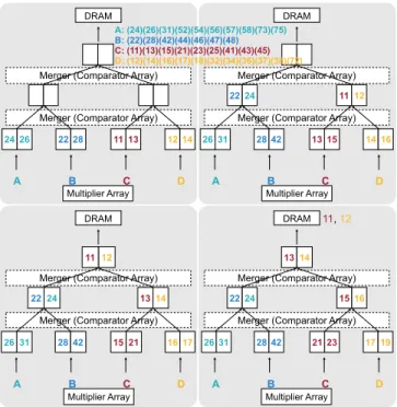
Figure 5. A merge tree which merges four partial product matrices. We only show coordinates of elements here.

each cycle.

2) Hierarchical Parallel Merge Unit: To increase the

merger parallelism, we can increase the size of the com-parator array, such as from 4×4 to 12×12. Nevertheless, the number of comparators isO(n2₎_{, where}_n_{is the side length}

of the comparator array, thus consuming a large number of hardware resources. Therefore, we further propose a hierarchical merger in Figure 4. We use two levels of comparator arrays to reduce the total number of comparators. The hierarchical merge unit contains high-level and low-level comparator arrays. We divide the input into chunks of 4, as in Figure 4 top. The length of each chunk equals to the input length of the low level comparator array (4 in the example). The top level array is used to decide which chunks need to be compared by low level arrays. The intuition is that if the largest element of chunk A is still smaller than chunk B, then we can skip the comparison of the two chunks. We use the top level comparator array to compare the last element in each chunk and get the boundary tiles (marked in red). Since each chunk is already sorted, the last element is the largest. The boundary tiles indicate the chunk pairs for the low level comparator arrays. For example, in Figure 4, the right-bottom tile is a boundary tile, so the A2 and B2 chunk is a chunk pair. We also divide the top level comparator array into diagonal groups, and each group will generate one and only one chunk pair. Then we use five low level comparator arrays to process the chunk pairs in parallel.

Output of each low level comparator array is limited by amin-max bound to avoid element duplication. Results not

First Matrix A

=

3 zero_count 0 0 1 2 2 2 3 iter1: if zero_count[0] == 1 shift left by 1 1 0 0 2 3 0 4 0 1 0 0 2 3 4 0 0 3 zero_count 0 0 1 2 2 2 2 iter2: if zero_count[1] == 1 shift left by 2 1 0 0 2 3 4 0 0 1 2 3 4 0 0 0 0 Ma tri x C on de nsi ng Round 0 Round 1 Round 2 Lo ad Se qu en ce

Matrix Condensing stored in CSR, loaded by condensed column 1st 4th 2nd 3rd Pipelined Multiply

and Merge Matrix Condensing Huffman Tree Scheduler Row Prefetcher 5.7x slowdown

Merger (Comparator Array)

26 31 28 42 13 15 14 16

22 24 11 12

DRAM

A

B

C

D

Multiplier Array

24 26 22 28 11 13 12 14

DRAM

A

B

C

D

26 31 28 42

22 24

15 21 16 17

13 14

11 12

DRAM

A

B

C

D

26 31 28 42 21 23 17 19

22 24 15 16

13 14

DRAM

A

B

C

D

11

,

12

Multiplier Array Multiplier Array Multiplier Array A: (24)(26)(31)(52)(54)(56)(57)(58)(73)(75) B: (22)(28)(42)(44)(46)(47)(48) C: (11)(13)(15)(21)(23)(25)(41)(43)(45) D: (12)(14)(16)(17)(18)(32)(34)(36)(37)(38)(72) Vanilla Inner Product Based

=

A

B

C

Vanilla Outer Product Based

=

Good Input Reuse

{

Poor Output Reuse

me rge ma ny part ial ma trice s

D

E

H

G

F

Proposed Outer Product Based

=

❹ Row Prefetcher

{

less me rge (1) (2)

J

K

E

D’

R8 A 15

A 15 B 15 C 13 D 12 E 9 F 7 G 3 H 2 I 2 J 2 K 2 L 2

weight

∝

memory access

(a)

C 28 B 15 13 A 15 E 9 17 K 2 L 2 4 I 2 J 2 4 8 32 F 7 5 12 G 3 H 2 12 D 24 52 84

R0 R2 R6 R5 R4 R1 R7 B 15 C 13 D 12 E 9 F 7 G 3 H 2 I 2 J 2 K 2 L 2

(b)

J 2 K 2 L 2 6 C 13 G 3 H 2 I 2 A 15 B 15 D 12 E 9 F 7 13 41 84 R0 R1 R2 R3 A 15 B 15 C 13 D 12 E 9 F 7 G 3 H 2 I 2 J 2 K 2 L 2

Total weight of all nodes reduces to: 228

(c)

A 4 D L K 2 7 C 2 I 9 4 13 16 17 33 5 J 2 B 2 G 15 16 15 H 2 F 3 20 31 51 84 E 12 0.6 1.3 2.2 1.1 Partial Matrix B Partial Matrix A 0.1 0.5 0.2 1.2

+

0.1 1.1 0.2 1.3 2.2 1.1 1.2

=

Merged (1, 0.1)(3, 1.1)(4, 0.2)(5, 1.3)(10, 2.2)(12, 1.1)(13, 0.1) Sorted (1, 0.1)(3, 0.5)(3, 0.6)(4, 0.2)(5, 1.3)(10, 2.2)(12, 1.1)(13, 0.1) 0 1 2 3 4 5 6 7 Comparator Array (1, 0.1) (3, 0.5) (4, 0.2)(13, 1.2) (3, 0.6) (5, 1.3) (10, 2.2) (12, 1.1) ≥ ≥ < ≥ ≥ ≥ ≥ ≥ ≥ ≥ ≥ ≥ 0 1 2 3 1 2 3 4 2 3 4 5 3 4 5 6,7 < < < < < < < < ≥ ≥ ≥ ≥ 3 4 5 6 4 5 6 7 4 5 6 7 A0 B0 < < < ≥ ≥ < ≥ ≥ ≥ 0 1 2 1 2 3 2 3 4

A0

(13,

1.2)

A1

(37,

9.2)

A2

(58,

-10.8)

B0

(12, 1.1)

B1

(40, 9.2)

B2

(61, 9.9)

D

eci

de

ch

un

k

Pa

irs

fo

r

lo

w

le

ve

l

co

mp

ara

to

r

arra

ys

B1 B1 A2 B1 A2 B2 0 1 2 3 4

Top level

comparator array

compares last element

in each chunk

Low level

comparator arrays

compare chunk pairs

in parallel

A0 A1

A0

B0

Zoom In

(1, 0.1) (3, 0.5) (4, 0.2)(13, 1.2) (3, 0.6) (5, 1.3) (10, 2.2) (12, 1.1) ≥ ≥ < ≥ ≥ ≥ ≥ ≥ ≥ ≥ ≥ ≥ 0 1 2 3 1 2 3 4 2 3 4 5 3 4 5 6,7 < < < < < < < < ≥ ≥ ≥ ≥ 3 4 5 6 4 5 6 7 4 5 6 7 (1,0.1)(3,0.5)(4,0.2)

Chunk A0

(13,1.2) (19,5.1)(22,-3.1)(35,1.2)(37,9.2)

Chunk A1

(42,1.1)(47,9.9)(48,0.3)(58,-10.8)

Chunk A2

Partial Matrix A

(3,0.6)(5,1.3)(10,2.2)(12,1.1)

Chunk B0

(15,4.4)(29,3.9)(35,-1.1)(40,9.2)

Chunk B1

(44,7.1)(52,-1.0)(55,0.2)(61,9.9)

Chunk B2

Partial Matrix B

R0-0

R0

R0-1

R0-2

R0-3

R0-4

R0-5

R0-6

R1-0

R1

R1-1

R1-2

R1-3

R2-0

R2

R2-1

R2-2

R2-3

R2-4

R2-5

R2-6

R2-7

R2-8

R2-9

R3-0

R3

R3-1

R3-2

R4-0

R4

R4-1

R4-2

R4-3

R4-4

R4-5

Replace R0

then

Replace R1

R1-0

R1-1

R1-2

R1-3

C1

R1-0

R1-1

R1-2

R1-3

R0-0

R0-1

R0-2

R0-3

R0-4

R0-5

R0-6

C0

R2-8

R2-9

R1-2

R1-3

R2-1

R2-2

R2-3

R2-4

R2-5

R2-6

R2-7

R2-0

C2

R2-8

R2-9

R3-0

R3-1

R2-1

R2-2

R2-3

R2-4

R2-5

R2-6

R2-7

R3-2

C3

Replace R1

then

Replace R2

R2-8

R2-9

R2-0

R3-1

R2-1

R2-2

R2-3

R2-4

R2-5

R2-6

R2-7

R3-2

C2

Replace

R3

R2-8

R2-9

R1-0

R3-1

R1-1

R1-2

R1-3

R2-4

R2-5

R2-6

R2-7

R3-2

C1

Replace

R2

R4-4

R4-5

R1-0

R3-1

R1-1

R1-2

R1-3

R4-0

R4-1

R4-2

R4-3

R3-2

C4

Replace

R2

R4-4

R4-5

R1-0

R3-1

R1-1

R1-2

R1-3

R4-0

R4-1

R4-2

R4-3

R3-2

C1

Replace

R4

R4-4

R4-5

R1-0

R3-1

R1-1

R1-2

R1-3

R3-0

R4-1

R4-2

R4-3

R3-2

C3

Replace R3

then

Replace R4

R0-6

R4-5

R1-0

R0-1

R1-1

R1-2

R1-3

R0-0

R0-3

R0-4

R0-5

R0-2

C0

R0-6

R4-5

R1-0

R0-1

R1-1

R1-2

R1-3

R0-0

R0-3

R0-4

R0-5

R0-2

C1

R0-6

R4-5

R1-0

R0-1

R1-1

R1-2

R1-3

R0-0

R0-3

R0-4

R0-5

R0-2

C0

C1

C0

C2

C3

C2

C1

C4

C1

C3

C0

C1

C0

C4

C1

C0

D

ist

an

ce

: 7

D

ist

an

ce

: 3

Step0

Step1

Step2

Step3

Step4

Step5

Step6

Step7

Step8

Step9

Step10

Step11

Row DistanceRow

PMat

Figure 6. Zero Eliminator. Bit 0 of zero count is checked to determine whether to shift by 1 in the first layer. Bit 1 ofzero countis checked to determine whether to shift by 2 in the second layer. We needlogN -cycle-latency to process input of length N.

in the bounds are set to 0. If the top level boundary tile has one left/top boundary tile neighbor, then the min bound is the first element of the top/left input chunk. The min bound of the first low level array is the smallest element. The max bound of each low level array is the min bound of the next one. The upper bound of the last low level array is+∞.

Then the outputs of each low level array are concatenated together to get the overall output. In this way, we save the low level comparators in non-boundary tiles in the high level array. Mathematically, the number of comparators is reduced to O(n43). If we choose a n23 ×n23 top level comparator array andn13×n13 low level comparators, we can processn elements at a time and uses only(2n23−1)∗(n13)2+(n23)2=

O(n43)comparators.

3) Merge Tree: Using the hierarchical merger, we get a

highly parallelized binary streaming merger that can merge up to 16 elements in each cycle. It merges two arrays into one array. In order to merge more arrays into one array, we stack multiple binary mergers and form a merge tree. As shown in Figure 5, the merge tree is a full binary tree that each node represents a FIFO on the hardware. Input arrays are fed to the leaf nodes, and the output array is collected from the root node. A binary merger merges the elements from the child FIFO and stores the results to the parent FIFO. The throughput of the whole tree is bounded by the root node, which has only one merger. Therefore, each layer

shares one merger to balance the throughput.

Figure 5 illustrates a merge tree of 2 layers, and each layer is equipped with a 1×1 merger. We only show coordinates of elements here. Four arrays A, B, C, D are to be merged. They are loaded into the leaf FIFOs. In the first 4 cycles, the lower merger merges data from the leaf FIFOs and store the results to the middle FIFOs. Then the upper merger notices there is enough data in the middle FIFOs, so it merges them and stores to the topmost FIFO. When the root FIFO is full, data is written to DRAM. The merge tree continues to working streamingly until all data fed to the lowest FIFO reach the root, and four arrays are merged fully on-chip.

4) Adders and Zero Eliminator: The merger stated above

only merges the elements and leaves alone same-location elements, i.e., elements with the same row and column index. However, in SpGEMM, we need to perform add operation on those elements. Therefore, we connect a slice of adders right after the merger, and it will add adjacent same-location elements and set one of the elements to zero. Then we use

(5)

First Matrix A

=

3 zero_count 0 01 2 2 23 iter1: if zero_count[0] == 1 shift left by 1 1 0 0 2 3 0 4 0 1 0 0 2 3 4 0 0 3 zero_count 0 0 12 2 2 2 iter2: if zero_count[1] == 1 shift left by 2 1 0 0 2 3 4 0 0 1 2 3 4 0 0 0 0 Ma tri x C on de nsi ng Round 0 Round 1 Round 2 Lo ad Se qu en ce

Matrix Condensing Stored in CSR; Loaded by condensed column 1st 4th 2nd 3rd Pipelined Multiply

and Merge Matrix Condensing

Huffman Tree

5.7x slowdown

1.5x speedup

26 31 28 42 13 15 14 16

22 24 11 12

A B C D

24 26 22 28 11 13 12 14

A B C D

26 31 28 42

15 21 16 17

13 14

11 12

26 31 28 42 21 23 17 19

22 24 15 16

13 14

Merger (Comparator Array) DRAM 11,12 Multiplier Array A: (24)(26)(31)(52)(54)(56)(57)(58)(73)(75) B: (22)(28)(42)(44)(46)(47)(48) C: (11)(13)(15)(21)(23)(25)(41)(43)(45) D: (12)(14)(16)(17)(18)(32)(34)(36)(37)(38)(72) Vanilla Inner Product Based

=

Good Input Reuse

{

Poor Output Reuse

=

❹ Row Prefetcher

❶ Pipelined Multiply and Merge ❷ Matrix Condensing Less Partial Matrices

{

A

1515B 13C 12D E 9F 7G 3H 22I J 2K 2L 2

weight

∝

memory access

(a)

C 28 B 15 13 A 15 E 9 17 K 2 L 2 4 I 2 J 2 4 8 32 F 7 5 12 G 3 H 2 12 D 24 52 84

R0 R2 R6 R5 R4 R1 R7 B 1513C 12D E 9F 7G 3H 22I J 2K 2L 2 (b)

Total weight of all nodes reduces to: 228

(c) A 4 D L K 2 7 C 2 I 9 4 13 16 17 33 5 J 2 B 2 G 15 16 15 H 2 F 3 20 31 51 84 E 12 0.6 1.3 2.2 1.1 Partial Matrix B Partial Matrix A 0.1 0.5 0.2 1.2

+

0.1 1.1 0.2 1.3 2.2 1.1 1.2

=

Merged (1, 0.1)(3, 1.1)(4, 0.2)(5, 1.3)(10, 2.2)(12, 1.1)(13, 0.1) Sorted (1, 0.1)(3, 0.5)(3, 0.6)(4, 0.2)(5, 1.3)(10, 2.2)(12, 1.1)(13, 0.1) 0 1 2 3 4 5 6 7 Comparator Array (1, 0.1) (3, 0.5) (4, 0.2) (13, 1.2) (3, 0.6) (5, 1.3) (10, 2.2) (12, 1.1) ≥ ≥ < ≥ ≥ ≥ ≥ ≥ ≥ ≥ ≥ ≥ 0 1 2 3 1 2 3 4 2 3 4 5 3 4 5 6,7 < < < < < < < < ≥ ≥ ≥ ≥ 3 4 5 6 4 5 6 7 4 5 6 7 A0 B0 < < < ≥ ≥ < ≥ ≥ ≥ 0 1 2 1 2 3 2 3 4 A0 (13, 1.2) A1 (37, 9.2) A2 (58, -10.8) B0 (12, 1.1) B1 (40, 9.2) B2 (61, 9.9) _Deci de ch un k Pa irs fo r lo w le ve l co mp ara to r arra ys B1 B1 A2 B1 A2 B2 0 1 2 3 4 Top level comparator array compares last element

in each chunk

in parallel A0 A1 A0 B0 Zoom In (1, 0.1) (3, 0.5) (4, 0.2) (13, 1.2) (3, 0.6) (5, 1.3) (10, 2.2) (12, 1.1) ≥ ≥ < ≥ ≥ ≥ ≥ ≥ ≥ ≥ ≥ ≥ 0 1 2 3 1 2 3 4 2 3 4 5 3 4 5 6,7 < < < < < < < < ≥ ≥ ≥ ≥ 3 4 5 6 4 5 6 7 4 5 6 7 (1,0.1)(3,0.5)(4,0.2) Chunk A0 (13,1.2) (19,5.1)(22,-3.1)(35,1.2)(37,9.2) Chunk A1 (42,1.1)(47,9.9)(48,0.3)(58,-10.8) Chunk A2 Partial Matrix A (3,0.6)(5,1.3)(10,2.2)(12,1.1)

Row DistanceRow

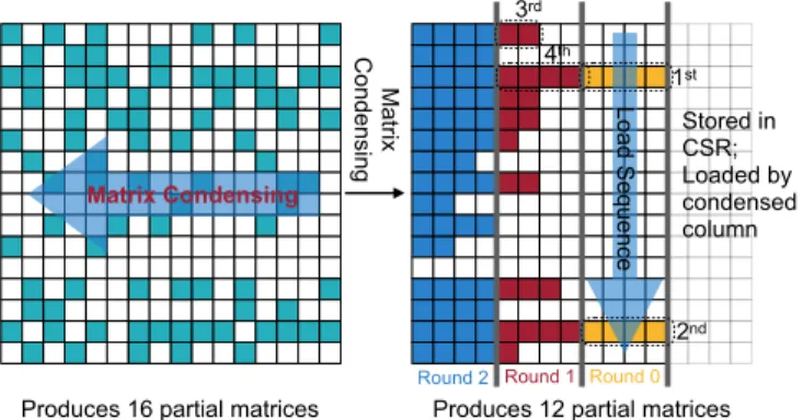
PMat Figure 7. Matrix Condensing. Condense the sparse matrix to the left,

reducing the number of columns, thus reducing the number of partial matrices. It can be stored naturally using the CSR format.

a Zero Eliminator to compress these zeroes and output the dense results. The Zero Eliminator consists of two parts. The first part is a prefix sum module that computes the number of zeroes (zero count) before each element. The second part is a modified logN layer shifter. Each layer contains N

MUXs that shift the input array andzero countby 1,2,4,... positions. Unlike a traditional shifter in which MUXs share a common control signal, the MUXs in Zero Eliminator are controlled by the zero count signal of each element. Figure 6 shows an example of the Zero Eliminator.

B. Matrix Condensing

Due to the limitation of hardware resources, we can only afford to merge 64 arrays on-chip. However, the intermediate results generated by the multiplier can be as large as 10,000 to 1,000,000, which requires multiple rounds of 64-way merging and still consumes a considerable amount of DRAM bandwidth. Therefore, we propose matrix condensing to merge multiple columns into a single column, which reduces the number of partial matrices to 100 to 1,000 in our benchmarks.

The motivation of matrix condensing is that if we have two columns a1, a2 from the left matrix that have no elements sharing the same row index, we can merge them (i.e., combine them into a new array sorted by the row index) while keeping the original column index. When we process the merged column in multiply phase, we multiply each element by its corresponding row (the same as its original column index) in the second input matrix B. The result is the same as the merge result of a1×B and a2×B. We

use a cheap merge of the left matrix to replace an expensive merge of the much longer multiplied results and reduce the number of partial matrices.

Furthermore, since exchanging elements between different columns does not affect the final result, we condense all elements in a row to the leftmost column. In this way, the number of columns of the condensed left matrix is far less than the original one. The number of partial product matrices is equivalent to the number of condensed columns, which is

reduced by three orders of magnitude.

Figure 7 shows a matrix in condensed format. The number of columns is reduced from 16 to 12, which equals the length of the longest row in the original matrix. In real-world datasets, we can reduce it from 100,000 to 100˜1,000, which is much closer to the size of the merge tree.

We store the left matrix in CSR format. The elements in CSR directly map to those in condensed format: theith

element in a CSR row is just in theith _{column of condensed}

format. CSR format and our condensed format are two different views of the same data. In the view of DRAM, the matrix is loaded by the rows, but in the view of a port of the merge tree, the matrix is loaded by condensed columns. This is achieved by the data loader, which dispatches data to different ports according to its condensed column. As in Figure 7, if the merger has parallelism of 4, we load four condensed columns together. The dash frames show the load sequence. After loading an element from the left matrix, we can use its original column index to fetch a row from the right matrix and fed them to the multipliers. The multiplied results will be fed to the ports whose index equals to the condensed column index (not the original column index).

C. Huffman Tree Scheduler

The merge unit can merge 64 matrices on-chip. After matrix condensing, the number of partial matrices can still exceed 64, which needs to be written to DRAM and merged later. The order of the merge matters: the earlier a matrix is merged, the more rounds of DRAM read and write it needs. Intuitively, we should merge sparser partial products matrices first, since they have less number of non-zeros; even in-and-out from DRAM for many times, the access number is smaller. We should leave denser matrices merged later. To wisely choose the order, we use a Huffman tree scheduler to minimize memory access during the whole task.

Our scheduler abstracts the entire merge process as a tree. In Figure 8, we show the 2-way and 4-way Huffman tree schedulers when the merger can merge 2, and 4 matrices at the same time. We also show a 2-way sequential scheduler without the Huffman tree scheduler for comparison.

The leaf nodes in the tree represent the initial multiplied results of a column in the left matrix with the right matrix. The internal nodes represent the partially merged results. The weights of the nodes represent the size of partially merged results or the size of the initial multiplied results. For internal nodes, we estimate its weight by adding up the weights of its children because the matrix is very sparse, and the additions during the merge stage are relatively rare. The arrow points from nodes to their parent node represent a round of multiply-and-merge operation.

The memory access amount of all partially merged results equals to the sum of all internal node weights. Since the root node and leaf node weights do not rely on the tree shape, the optimization goal is to minimize the total weights of

(6)

and Merge Matrix Condensing

Huffman Tree

5.7x slowdown

26 31 28 42 13 15 14 16

2224 11 12

A B C D

24 26 22 28 11 13 12 14

A B C D

26 31 28 42

22 24

15 21 16 17

1314

11 12

A B C D

26 31 28 42 21 23 17 19

2224 1516

1314

Merger (Comparator Array) DRAM A B C D 11, 12 Multiplier Array Multiplier Array Multiplier Array A: (24)(26)(31)(52)(54)(56)(57)(58)(73)(75) B: (22)(28)(42)(44)(46)(47)(48) C: (11)(13)(15)(21)(23)(25)(41)(43)(45) D: (12)(14)(16)(17)(18)(32)(34)(36)(37)(38)(72) Vanilla Inner Product Based =

Good Input Reuse

{

Poor Output Reuse me rge ma ny part ial ma trice_s D E H G F Proposed Outer Product Based =

❹ Row Prefetcher

{

less me rge (1) (2) J K E D’ R8 A 15 2-Way with Sequential Scheduler

Total weight of all nodes: 365 A 15 B 15 C 13 D 12 E 9 F 7 G 3 H 2 I 2 J 2 K 2 L 2

weight∝memory access (a)

C 28 B 15 13 A 15 E 9 17 K 2 L 2 4 I 2 J 2 4 8 32 F 7 5 12 G 3 H 2 12 D 24 52 84

J 2 K 2 L 2 6 C 13 G 3 H 2 I 2 A 15 B 15 D 12 E 9 F 7 13 41 84 R0 R1 R2 R3 A 15 B 15 C 13 D 12 E 9 F 7 G 3 H 2 I 2 J 2 K 2 L 2

Total weight of all nodes reduces to: 228 (c) A 4 D L K 2 7 C 2 I 9 4 13 16 17 33 5 J 2 B 2 G 15 16 15 H 2 F 3 20 31 51 84 E 12 0.6 1.3 2.2 1.1 Partial Matrix B Partial Matrix A 0.1 0.5 0.2 1.2 + 0.1 1.1 0.2 1.3 2.2 1.1 1.2 = Merged (1, 0.1)(3, 1.1)(4, 0.2)(5, 1.3)(10, 2.2)(12, 1.1)(13, 0.1) Sorted (1, 0.1)(3, 0.5)(3, 0.6)(4, 0.2)(5, 1.3)(10, 2.2)(12, 1.1)(13, 0.1) 0 1 2 3 4 5 6 7 Comparator Array (1, 0.1)(3, 0.5)(4, 0.2)(13, 1.2) (3, 0.6) (5, 1.3) (10, 2.2) (12, 1.1) ≥ ≥ < ≥ ≥ ≥ ≥ ≥ ≥ ≥ ≥ ≥ 0 1 2 3 1 2 3 4 2 3 4 5 3 4 5 6,7 < < < < < < < < ≥ ≥ ≥ ≥ 3 4 5 6 4 5 6 7 4 5 6 7 A0 B0 < < < ≥ ≥ < ≥ ≥ ≥ 0 1 2 1 2 3 2 3 4 A0 (13, 1.2) A1 (37, 9.2) A2 (58, -10.8) B0 (12, 1.1) B1 (40, 9.2) B2 (61, 9.9) _Deci de ch un k Pa irs fo r lo w le ve l co mp ara to r arra ys B1 B1 A2 B1 A2 B2 0 1 2 3 4 Top level comparator array compares last element

in each chunk

in parallel A0 A1 A0 B0 Zoom In (1, 0.1) (3, 0.5)(4, 0.2)(13, 1.2) (3, 0.6) (5, 1.3) (10, 2.2) (12, 1.1) ≥ ≥ < ≥ ≥ ≥ ≥ ≥ ≥ ≥ ≥ ≥ 0 1 2 3 1 2 3 4 2 3 4 5 3 4 5 6,7 < < < < < < < < ≥ ≥ ≥ ≥ 3 4 5 6 4 5 6 7 4 5 6 7 (1,0.1)(3,0.5)(4,0.2) Chunk A0 (13,1.2) (19,5.1)(22,-3.1)(35,1.2)(37,9.2) Chunk A1 (42,1.1)(47,9.9)(48,0.3)(58,-10.8) Chunk A2 Partial Matrix A (3,0.6)(5,1.3)(10,2.2)(12,1.1)

Row DistanceRow MatA Element MatB Row Merger Merger New PMat Merger FIFO Partial Mat Fetcher Partial Mat Addr

Partial Mat Writer Old PMat Figure 8. Huffman tree scheduler gives near optimal order of partial matrices merging. The total memory access is minimized. The weights of nodes represent the number of non-zeros in the partial matrix. The total DRAM access is proportional to the sum of nodes’ weights.

all nodes, which also equals the sum of the weights of leaf nodes multiplied by their depths in the tree.

A k-ary Huffman Tree is proven to be the optimal solution to minimize the sum of all nodes. It puts larger leaf nodes nearer to the root and smaller nodes farther, so the accu-mulative products of weights and depths can be minimized. This is exactly what we need to minimize the total DRAM traffic. In each round of the Huffman Tree construction, we select k un-merged nodes withminimal weights and merge them into an internal node except the first round. In the first round, the number of nodes that need to choose can be calculated with Formula 1. This guarantees that the last round always merges k nodes, so the root node of the tree isalways full.

kinit= (numcondensed col−2)mod(nummerger way−1)+2

(1) In the example (Figure 8), a 2-way Huffman scheduler reduced the total weights from 365 to 354. A 4-way Huff-man scheduler further reduces it to 228. The weight is proportional to the DRAM traffic. Therefore total weight is reduced when the parallelism of the merger increases. However, high parallelism usually comes at the cost of high power consumption and large area. We choose a 64-way Huffman tree scheduler, and will discuss the trade-offs in Section III.

In our real implementation, the Huffman tree is built on the fly with a priority queue. The implementation reflects the algorithm of building a Huffman tree. We firstly add the weights of leaf nodes to the queue and sort them. For a

m−way merger, in each iteration, the firstmpartial matrices are merged, and the weight of the merged matrix is added to the queue, and then we sort the queue again.

D. Row Prefetcher

Matrix condensing reduces the number of partial matrices but ruins the input reuse of the second operand matrix since one column after condensing requires the elements from

different rows of the second matrix. We solve the problem by a row prefetcher with near-optimal buffer replacement.

The prefetcher is motivated by the fact that we can predict the access order of the right matrix ahead of time. As mentioned in section II-B, we access the left matrix from top to down. Using the column index of the left matrix, we can deduce the order of the right matrix, which can be used by the prefetcher to load data before they are consumed by the multipliers.

The prefetcher has two functions: first, fetching the data used by multipliers ahead of time to hide the latency of DRAM; second, caching the fetched data in a buffer for future reuse to reduce the amount of DRAM reading.

The first function is achieved by multiple data fetchers. We use a data fetcher for each DRAM channel. Accesses to different DRAM channels and banks are overlapped; thus, the DRAM latency can be hidden.

The second function is achieved by an on-chip buffer, which stores the rows of the right matrix. When new data is fetched, using the predicted access order, we can replace the line with the furthest next use, which can achieve near-optimal reuse if the prediction is accurate.

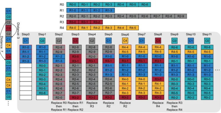
In Figure 9, we show a simplified example. The left column is one condensed column from the condensed first matrix. Each element is marked with its original column. The first three are original column 1, 0, and 2. On the top, we show row 0 to row 4 of the second matrix and divide them according to the length of the buffer line. The central part of the figure shows the buffer at different time steps. The red frames highlight the new contents after each time step.

In time step 0, we load Row 1. In time step 1, we load Row 0. In time step 2, we firstly store R2-0. Then we need to spill some buffer lines to continue to load R2. We spill R0 first because R0 will be used in 7 time steps later, and R1 will be used in 3 time steps later. However, after spilling all R0 lines, R2 still has remaining parts. So we have to spill

(7)