Mining the Bilinear Structure of Data with
Approximate Joint Diagonalization
Louis Korczowski, Florent Bouchard, Christian Jutten, Marco Congedo
To cite this version:
Louis Korczowski, Florent Bouchard, Christian Jutten, Marco Congedo. Mining the Bilinear
Structure of Data with Approximate Joint Diagonalization. 24th European Signal Processing
Conference (EUSIPCO 2016), Aug 2016, Budapest, Hungary. 24th European Signal Processing
Conference (EUSIPCO), pp.667-671, 2016.
<
hal-01357245
>
HAL Id: hal-01357245
https://hal.archives-ouvertes.fr/hal-01357245
Submitted on 29 Aug 2016
HAL
is a multi-disciplinary open access
archive for the deposit and dissemination of
sci-entific research documents, whether they are
pub-lished or not.
The documents may come from
teaching and research institutions in France or
abroad, or from public or private research centers.
L’archive ouverte pluridisciplinaire
HAL
, est
destin´
ee au d´
epˆ
ot et `
a la diffusion de documents
scientifiques de niveau recherche, publi´
es ou non,
´
emanant des ´
etablissements d’enseignement et de
recherche fran¸
cais ou ´
etrangers, des laboratoires
publics ou priv´
es.
Mining the Bilinear Structure of Data with
Approximate Joint Diagonalization
Louis Korczowski, Florent Bouchard, Christian Jutten, Marco Congedo
GIPSA-lab, Univ. Grenoble Alpes, CNRS, Grenoble Institute of Technology, Grenoble FranceEmail: [email protected]
Abstract—Approximate Joint Diagonalization of a matrix set can solve the linear Blind Source Separation problem. If the data possesses a bilinear structure, for example a spatio-temporal structure, transformations such as tensor decomposition can be applied. In this paper we show how the linear and bilinear joint diagonalization can be applied for extracting sources according to a composite model where some of the sources have a linear structure and other a bilinear structure. This is the case of Event Related Potentials (ERPs). The proposed model achieves higher performance in term of shape and robustness for the estimation of ERP sources in a Brain Computer Interface experiment.
I. INTRODUCTION
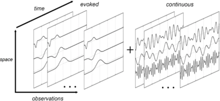
Event-Related Potentials (ERPs) are transient brainwaves with a fixed evoked spatio-temporal pattern ; their polarity, shape, latency and amplitude are approximatively constant across observations for a given class of stimuli evoking them. The amplitude of ERPs is known to be very low compared to the ongoingcontinuousbackground activity of the brain. For many applications such as classification or clinical analysis, one would like to retrieve bothevokedandcontinuoussources of the brain (Figure 1).
Blind Source Separation (BSS) is a fundamental framework for modeling independent sources hidden in the observations. BSS methods find major applications in telecommunication, biomedical engineering, speech, audio and video processing [1].
Let us consider the instantaneous linear mixture given by
x(t) =As(t) +n(t), (1) wheretis the time index,x(t),s(t)∈RN are respectively the observation and source vectors,A ∈ RN×N is an invertible
unknownspatial mixing matrix, andn(t)∈RN is an additive
noise vector. In model (1) the fixed pattern is only spatial. We can formulate the problem of estimatings(t)by finding a
spatial unmixing matrix Bthat solvessˆ(t) =BTx(t) where
the sources ˆs = P∆s are estimated up to a permutation matrix P and a diagonal matrix (scaling) ∆ ambiguity ; superscript(.)T is the transpose operator.
Approximate Joint Diagonalization (AJD) is a class of meth-ods for solving the BSS problem relying on the diagonalization of a set of symmetric matricesRx(l)∀l∈ {1, ..., L}, named targetmatrices, containing statistics of the observationx. The choice of the statistics (e.g. correlations, time-lagged covari-ances, co-spectra, higher order cumulants, etc.) depends on assumptions on the sources such as non-stationarity, spectral coloration, non-Gaussianity, etc. [1], [2]. Indices l can stand,
Fig. 1. Thecompositemodel assumes that the observations are the superpo-sition of evoked sources and continuous sources linked by the same spatial mixing matrixA.
e.g., for delaysτ in the case of covariances or for frequencies
f in the case of co-spectra, etc. [2]. Thus, the BSS problem can be reformulated as
Rx(l) =ARs(l)AT , (2)
where Rs(l) is a diagonal matrix containing the power of
the sources. We seek a matrixB that jointly diagonalizes all matricesRx(l) in (2)as much as possible(i.e., according to
some criterion)
Rˆs(l) =BTRx(l)B . (3)
AJD has been successfully used in source separation of
continuous electroencephalographic (EEG) sources [3] using co-spectral astarget matrices. More recently, [4] proposed to add the covariance matrices of the estimated evoked activity for the separation of Event Error Related Potential (ErrP) sources. In ERPs, theevoked sources have both a spatial and a temporal (bilinear) fixed structure such as
Xk=ASkET +Nk , (4)
where matricesXk ∈RN×T are a set of observation matrices withk∈ {1, ..., K},E∈RT×N is an unknowntemporal
mix-ing matrix andSk ∈RN×N is a diagonal matrix containing the amplitude of the sources andNk∈RN×T is a noise term. The difference with the linear BSS case (1) is that the bilinear model has now also a fixed temporal structure, contained in
E, which can be modulated in amplitude across observations bySk. It is a bilinear BSS problem with
ˆ
where now two unmixing matricesB andD are required for diagonalizing as much as possibleSˆk. A proposed algorithm
solved it by Approximate Joint Singular Value Decomposition (AJSVD) in [5] consideringAandE orthogonal. More gen-erally, the model can be solved by tensor rank decomposition, i.e. Candecomp/PARAFAC (CP) [6].
Such model was used for the extraction of the ERP sources in functional Magnetic Resonance Imaging (fMRI) [7] and a solution using AJD was proposed in [8] by diagonalizing both spatial and temporal covariance matrices. Recently, CP decom-position was used in addition to Extended Kalman Filter in [9] with successful estimation of the electroencephalographic ERP at single trial level.
However, in real data such as ERP, the observation Xk is
an additive process (see Figure 1) of both continuousactivity which is separable by the linear model (3), andevokedactivity, which is separable by the bilinear model (5). Thus trying a linear BSS (respectively bilinear BSS) method to extract the
continuous(respectivelyevoked) sources will fail because the model neglects the contribution of the evoked (respectively
continuous) sources. Eventually none of these models can find the trueunmixing matrices B,D.
To go beyond those limitations, we propose in Section II-A a composite model that can be used to solves simultaneously the AJD for (1) and a bilinear AJD (BAJD) for (4). We name the proposed model composite AJD (CAJD). We give the corresponding cost functions for AJD, BAJD and CAJD in Section II-B and a closed-form minimizer of the respective cost function by Gauss Planar Transformation (GTP) in Sec-tion II-C, using yet a novel Jacobi-like algorithm. We compare the proposed models in the estimation of matrices B andE
on simulated data in Section III-A and we compare BAJD vs. CAJD on EEG ERP in Section III-C.
II. METHODS
A. Composite Approximate Joint Diagonalization
One would like to complete the full source separation by jointly diagonalize BTRx(l)B and BTXkD where B and
Dare respectively the spatial and temporal unmixing matrices supposed invertible. Note that ifEin model (4) is furthermore supposed orthogonal and its estimation is not of interest for the user, one can always consider the classical AJD framework as
XkXkT =ASkEETSkAT =ARs(k)AT ∀k ∈ {1, ..., K}
(withSk diagonal), coming back to (2).
B. Cost Functions
In the linear model case given by (3) and using the standard AJD framework, we consider the cost functionf,
f(B) = L X l=1 off(BTRx(l)B) 2 F , (6)
where matrices Rx(l) correspond to the chosen statistics of
Xkandoff(.)is the off-diagonal operator that set all diagonal
elements of the argument to zero.
For the bilinear model (4), BAJD uses a similar cost function fb, where bstand for bilinear, given by
fb(B,D) = K X k=1 off(BTXkD) 2 F , (7)
where matrices Xk correspond to observations in
spatio-temporal domain (i.e., for ERP, the raw potential and not their covariance) andBandDare their corresponding spatial and temporal unmixing matrices, respectively.
Finally for the composite model introduced in the previous section, the corresponding cost function fc, where cstand for composite, is given by
fc(B,D) =αf(B) + (1−α)fb(B,D), (8)
whereα∈[0,1]is a fixed ponderation weight which expresses a preference among the two models if α 6= 0.5, i.e linear (>0.5) or bilinear (<0.5). In this work, we considerα= 0.5.
C. Optimization by Gauss Planar Transformations
To solve the problem for the three functions we consider, we propose a novel optimization scheme inspired by eigenvector Jacobi and elementary Gauss elimination methods, named Gauss Planar Transformation (GPT). Note that we choose the same optimization scheme for all methods in order to compare the models fairly. Starting from initial guess matricesBandD
(see Section II-D), we perform repeated planar non-orthogonal transformations on the columns of the unmixing matrices. Giveniandj in{1, .., N}withi6=j, a(i, j)-transformation is defined as
bi ← bi+βbj
di ← di+γdj
where bi (respectively di) denotes the ith column of B
(respectivelyD). A sweep of the algorithms is then to perform
(i, j)-transformations for all iandj in{1, .., N} withi6=j. We seek parametersβ andγ that minimize the cost function for each(i, j)-transformation. Such a transformation acts only on the rowi and the column i of the matrices Rx(l)and/or
Xk. A solution would then to find β and γ in order to
minimize all those elements (except the diagonal one) as it is done in [10]. Another way is to only minimize the elements
(i, j)and (j, i)as in [11]. We choose the latter approach as this solution always converges faster and does not affect the performance (data not shown). Given i and j, this leads, in the AJD case (3), to minimize
fij(β) = 2 L P l=1 ((bT i +βbTj)Rx(l)bj)2
For the BAJD model in (5), we have to minimize
fijb(β) = K P k=1 ((bTi +βbTj)Xkdj)2 fijb(γ) = K P k=1 (bT jXk(di+γdj))2.
Finally, if we consider the CAJD model proposed in Section II-A, the functionals to minimize are
fijc (β) = (1−α) K P k=1 ((bT i +βbTj)Xkdj)2 + 2α F P f=1 ((bT i +βbTj)Rx(l)bj)2 fijc(γ) = (1−α) K P k=1 (bT jXk(di+γdj))2 .
All those functions are second order polynomials with closed form minimizers. Thus, for AJD with cost function (6), the optimalβ is given by β = K P k=1 (bT iRx(l)bj)(bTjRx(l)bj) K P k=1 (bT jRx(l)bj)2 .
For the BAJD model with cost function (7), optimalβ andγ
are given by β = K P k=1 (bT iXkdj)(bTjXkdj) K P k=1 (bT jXkdj)2 γ = K P k=1 (bTjXkdi)(bTjXkdj) K P k=1 (bT jXkdj)2 .
Finally, for our composite model CAJD with the cost function (8), optimal β andγ are given by
β= (1−α) K P k=1 (bTiXkdj)(bTjXkdj)+2α F P f=1 (bTiRx(l)bj)(bTjRx(l)bj) (1−α) K P k=1 (bT jXkdj)2+2α F P f=1 (bT jRx(l)bj)2 γ= K P k=1 (bT jXkdi)(bTjXkdj) K P k=1 (bT jXkdj)2 . D. Initialization
The initialization is of paramount importance for Jacobi-like algorithms. While a working initialization can be the identity matrix, we use singular value decomposition:
¯
XT =UΛVT , (9)
where X¯ is an estimation of the evoked activity such as the arithmetic average X¯ = PK k 1 KXk or by regression based estimation [12]. We set ( B0=U D0= ˜VT (10)
where V˜ ∈ RT×N is the reduced right-handed component of the SVD-decomposition containing only the N singular vectors with the largest N associated singular values inΛ.
III. RESULTS
A. Simulations
In order to estimate the performances of CAJD compared to AJD and BAJD on the model that we consider, we first performed simulations within Matlab (c) environnement.
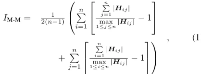
To analyze the quality of the spatial and temporal unmixing matrices found by both methods, we use the Moreau-Macchi indexIM-M [13] defined as IM-M= 2(n1−1) n P i=1 n P j=1 |Hij| max 1≤j≤n|Hij| −1 + n P j=1 n P i=1 |Hij| max 1≤i≤n|Hij| −1 , (11)
where H equals BTA (respectively ETD), with B
(re-spectively D) the estimated spatial (respectively temporal) unmixing matrix and A (respectively E) the true spatial (respectively temporal) mixing matrix.
We generatedK= 100 matricesXk of dimension N×T
withN = 16andT = 128 according to
Xk =ASkET +σNk , (12)
where A is the spatial mixing matrix being non-orthogonal generated randomly with i.i.d. elements normaly distributed
N(0,1).E is the temporal mixing matrix with i.i.d. elements generated from a multivariate normal distribution with a ran-dom covariance matrix. We controlled the non-orthogonality of A and E by constraining their condition number with respect to inversion between 1 and 20 (excluded). Matrices
Sk are diagonal with i.i.d. elements randomly drawn from a
normal distributionN(0,1).σis a free parameter defining the noise level and Nk are noise matrices with elements drawn
independently from a normal distributionN(0,1).
In parallel, we generated L = 100 matrices Rx(l) of
dimensionN×N according to Rx(l) =ARs(l)AT + σ2 2 (Nl+N T l ),
where A and σ are the same as before. Matrices Rs(l) are
diagonal with i.i.d. elements generated from a chi-squared distribution with two degrees of freedom. The symetrized noise matrices Nl are with elements drawn independently
from a normal distribution N(0,1).
AJD was performed on the matrices XkXkT and Rx(l)
Fig. 2. Moreau-Macchi criteria on the matrixB. Average performance of GPT algorithms on 100 independant realizations (a) without noise (σ = 0) and (b) with noise (σ= 0.1).
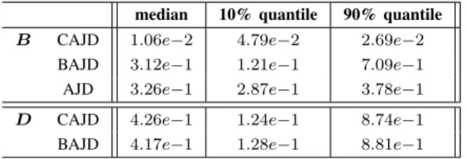
TABLE I
MOREAU-MACCHICRITERION AFTER CONVERGENCE. 100INDEPENDENT DRAWS OF MATRICESAANDEWITHσ= 0.1.
median 10% quantile 90% quantile
B CAJD 1.06e−2 4.79e−2 2.69e−2
BAJD 3.12e−1 1.21e−1 7.09e−1
AJD 3.26e−1 2.87e−1 3.78e−1
D CAJD 4.26e−1 1.24e−1 8.74e−1
BAJD 4.17e−1 1.28e−1 8.81e−1
and B was initialized with the identity matrix. BAJD was performed on the matricesXk.Bwas initialized in the same
way as AJD and D with an orthogonalized random matrix. CAJD was performed on both the matrices Xk and Rx(l)
with the same initialization as BAJD.
As expected, becauseE is far from being orthogonal, AJD gives results far from the true solution, see Figure 2. Moreover, while we can not differentiate the performance of BAJD and CAJD in the case of no noise, the convergence is always better for CAJD is presence of noise for the estimation of
B (see Table I). The difference in the estimation of E is not significant between BAJD and CAJD because the simulated data respect the bilinear model.
Thus, CAJD displays overall better performances as com-pared to both AJD and BAJD on the estimation of B. Our model is equivalent to BAJD for the estimation of D. Next, we will test both BAJD and CAJD on real data.
B. Procedures
1) Data Acquisition: EEG signals were acquired during sessions of two subjects playing simultaneously to a P300-based BCI [14]. EEG data were acquired with 32 active wet electrodes using USBamp amplifiers [g.Tec, Graz, Austria] with a sample rate Fs=512 Hz. Ground was an active electrode on Fz and reference was a passive electrode clip on the right earlobe. The ERP triggers were synchronized with the signals with a supplementary analog channel to minimize the jitter.
2) Preprocessing: From the recorded signals, we se-lected 16 representative electrodes from the first subject (N=16): Fp1-Fp2-F5-AFz-F6-T7-Cz-T8-P7-P3-Pz-P4-P8-O1-Oz-O2. The signals were filtered by a fourth order forward-backward Butterworth band pass filter [1-20] Hz and down-sampled at Fs=128Hz. The signals were segmented into trials
Xkof 1s (T=128) starting at each visual stimulation. Each trial
was labeled as TARGET (TA), i.e. with possible appearence of P300 potential, or NON-TARGET (NT) for the two different experimental conditions.
3) Target Matrices: We propose to estimate the evoked
activity X¯z by arithmetic ensemble average ofXk by
boot-strapping 50 new ensembles: 40 ensemble averages of 50 observations in the condition TA; 10 ensemble averages of 50 observations in the condition NT.
Thus for AJD (6), we propose target matrices Rx(l) ∈
{CX¯z,Cf} whereCf are co-spectral matrices computed by Bartlett’s average [15] over theKobservations for frequencies
Fig. 3. Left: columns ofEˆinormalized with L2-norm. Right: columns ofAˆi projected on a topographic scalp map in absolute amplitude and normalized with . Highlight : Sourcec06corresponds to P3b, sourcec11corresponds to early visual complex.
of interest, i.e. f ∈ {1,1.5,2, ...20}Hz for a total of 39 co-spectral matrices. CX¯z are the empirical covariance matrices
of the X¯z∀z ∈ {1, ...,50}. For BAJD (7), we diagonalized
¯
Xz . Eventually, for CAJD we replaceXk byX¯z andRx(l)
byCf in (8).
4) GPT initialization: The initialization ofB,Dwas made by a SVD step such as proposed in Section II-D with X¯
estimated with the method in [12] (no subspace reduction).
C. ERP Source Estimation
1) Source Separation: To asses the quality of the source separation obtained by CAJD, we compared the estimated sources according to their spatial and temporal contributions. We projected the columns ofAˆ=B−1on a scalp topographic map. The temporal source pattern is given by the columns
ˆ
E =D+ where superscript (.)+ denotes the Moore-Penrose pseudoinverse.
In Figure 3, we present the resulting estimation obtained by CAJD on a representative subject of our dataset. By visual inspection, we can observe that several sources correspond to
evoked potential: a)c11, the early visual complex, generated in the occipital (visual) cortex. This is common to conditions TA and NT but with a much lower amplitude in NT. b) c06
the P3b component of the ERP generated in parietal locations and with maximum amplitude around 300ms after the stimulus [16].
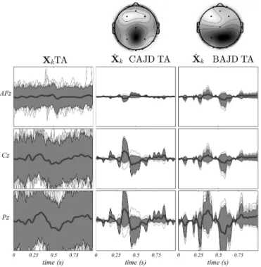
2) Source Quality: We focus on the quality of the estimated source associated to the evoked activity P3b of BAJD and CAJD in condition TA. Figure 4 displays their respective estimation (described in the following) at the single trial level and they are compared to the observationXk.
Fig. 4. TA condition: DataXk(left) and backprojected P3b source (13) for CAJD (center) and BAJD (right). Their respective spatial distribution is shown on top. y-axis are in relative amplitude. Thin grey line: observation (K=100). Thick black line: Ensemble average. Grey area: 10% and 90% quantiles, greater is the area, larger is the variability.
For a given observationXk, we estimated the corresponding
power of the sources in Sˆk and backprojected thei-th source
in the electrode domain such as: ˆ
Xk,i = ˆAiSˆkEˆiT (13)
where Xˆk,i is the projection of the i-th component in the
sensor domain. Aˆi and Eˆi are respectively the spatial and
temporal contributions of the i-th estimated component. The projected activity of the source P3b in Figure 4 shows that the sign and shape of the source is properly estimated for both methods. The polarity of the estimated P3b of CAJD is consistant over condition TA while it is not for condition NT (data not shown here). Interestingly, the CAJD is more robust to outliers as compared to BAJD, particulary in the early and late latency (before 250ms and after 700ms). Under this evidence, CAJD seems to estimate much better the real (physiological) source of the P3b.
IV. CONCLUSION
We have described a new approach for extracting event-related sources by mining the bilinear (spatio-temporal) struc-ture of the data with a composite model of both AJD and BAJD named Composite Approximate Joint Diagonalization (CAJD). We proposed to minimize the off-diagonal criteria by a novel algorithm, i.e. Gauss Planar Transformation (GPT). We provided the close-form approximate minimizer for the three models in the framework of GPT. CAJD achieves better performance than AJD and BAJD models on simulated data.
Moreover this method is relevant for single trial source extrac-tion in the case of Event-Related Potentials. We believe that CAJD could be applied on various situations such as denoising or classification for Brain Computer Interfaces. Eventually, the CAJD is not restricted to brain data but can be used for all combinaison of linear and bilinear structure whenever their relation is known.
ACKNOWLEDGMENT
This research is partly supported by the ERC CHESS (2012-ERC-AdG-320684). F. Bouchard is partially supported by the LabEx PERSYVAL-Lab (ANR-11-LABX-0025-01). We also thanks A. Andreev, engineer in charge of the software plate-form, and E. Ostaschenko, M. Cederhout for the experimental support.
REFERENCES
[1] Pierre Comon and Christian Jutten. Handbook of Blind Source Sepa-ration: Independent Component Analysis and Applications. Academic Press, February 2010.
[2] F.J. Theis and Y. Inouye. On the use of joint diagonalization in blind signal processing. In2006 IEEE International Symposium on Circuits and Systems, 2006. ISCAS 2006. Proceedings, pages 4 pp.–3589, 2006. [3] Marco Congedo, Cdric Gouy-Pailler, and Christian Jutten. On the blind source separation of human electroencephalogram by approximate joint diagonalization of second order statistics. Clinical Neurophysiology, 119(12):2677–2686, December 2008.
[4] Marco Congedo, Sandra Rousseau, and Christian Jutten. An Introduction to EEG Source Analysis with an Illustration of a Study on Error-Related Potentials. In Eduardo Reck Miranda and Julien Castet, editors,Guide to Brain-Computer Music Interfacing, pages 163–189. Springer London, January 2014.
[5] M. Congedo, R. Phlypo, and Dinh-Tuan Pham. Approximate Joint Singular Value Decomposition of an Asymmetric Rectangular Matrix Set. IEEE Transactions on Signal Processing, 59(1):415–424, January 2011.
[6] Tamara G. Kolda and Brett W. Bader. Tensor decompositions and applications. SIAM review, 51(3):455–500, 2009.
[7] J. V Stone, J Porrill, N. R Porter, and I. D Wilkinson. Spatiotemporal Independent Component Analysis of Event-Related fMRI Data Using Skewed Probability Density Functions. NeuroImage, 15(2):407–421, February 2002.
[8] F.J. Theis, P. Gruber, I.R. Keck, A. Meyer-Base, and E.W. Lang. Spatiotemporal blind source separation using double-sided approximate joint diagonalization. In Signal Processing Conference, 2005 13th European, pages 1–4, September 2005.
[9] Mohammad Niknazar, Hanna Becker, Bertrand Rivet, Christian Jutten, and Pierre Comon. Blind source separation of underdetermined mixtures of event-related sources. Signal Processing, 101:52–64, August 2014. [10] Xiao-Feng Gong, Xiu-Lin Wang, and Qiu-Hua Lin. Generalized
Non-Orthogonal Joint Diagonalization With LU Decomposition and Succes-sive Rotations. IEEE Transactions on Signal Processing, 63(5):1322– 1334, March 2015.
[11] V. Maurandi and E. Moreau. A Decoupled Jacobi-Like Algorithm for Non-Unitary Joint Diagonalization of Complex-Valued Matrices. IEEE Signal Processing Letters, 21(12):1453–1456, December 2014. [12] Marco Congedo, Louis Korczowski, Arnaud Delorme, and Fernando
Lopes da Silva. Spatio-temporal common pattern: A companion method for ERP analysis in the time domain.J. Neurosci. Methods, 267:74–88, April 2016.
[13] E. Moreau and O. Macchi. New self-adaptative algorithms for source separation based on contrast functions. In , IEEE Signal Processing Workshop on Higher-Order Statistics, 1993, pages 215–219, 1993. [14] Louis Korczowski, Alexandre Barachant, Anton Andreev, Christian
Jutten, and Marco Congedo. Brain Invaders 2 : an open source Plug & Play multi-user BCI videogame. In6th International Brain-Computer Interface Meeting, page 224, Pacific Grove, CA, United States, May 2016. BCI Society.
[15] M. S. Bartlett. Smoothing Periodograms from Time-Series with Con-tinuous Spectra. Nature, 161:686–687, May 1948.
[16] John Polich. Updating P300: An Integrative Theory of P3a and P3b.