Competing Distribution Classes
Dissertation zur Erlangung des Doktorgrades der
Naturwissenschaften (Dr. rer. nat.)
Fakultät Naturwissenschaften
Universität Hohenheim
Institut für Angewandte Mathematik und Statistik
Erscheinungsjahr: 2016
1.berichtende Person: Prof. Dr. Uwe Jensen
2.berichtende Person: Prof. Dr. Harro Walk
Mündliche Prüfung am: 2016/08/18
Firstly, I would like to express my sincere gratitude to my advisor Prof. Dr. Uwe Jensen for the continuous support of my Ph.D study and related research, for his patience, motivation, and immense knowledge. His guidance helped me in all the time of research and writing of this thesis.
My sincere thanks also goes to Dr. Maik Döring, Dr. André Erhardt, and Dr. Torsten Stefan for their insightful comments and encouragement. Last but not the least, I would like to thank the DFG (German Research Foundation) for the support and funding of the research project (Ge: Je 162 / 10-1, Schi 457 / 12-1).
1 Introduction 1
1.1 The Problem . . . 1
1.2 Notations . . . 5
1.3 Maximum Likelihood Theory . . . 6
1.4 Censored Data . . . 8
1.5 Kernel Estimate for Conditional Distribution Function . . . 10
2 Model Selection Testing 13 2.1 Notations and Hypotheses . . . 14
2.2 The Case with Number of Observations at Each Covariate Tend-ing to Infinity . . . 17
2.3 The Case with Number of Covariates Tending to Infinity . . . . 36
3 The Case with Right Censoring 51 3.1 Notations and Hypotheses . . . 52
3.2 The Case with Number of Observations at Each Covariate Tend-ing to Infinity . . . 55
3.3 The Case with Number of Covariates Tending to Infinity . . . . 66
4 Case Study 79 5 Simulation Studies 81 5.1 Comparing Two Weibull Classes . . . 82 5.2 Comparing Two Weibull Classes with Two Dimensional Covariate 84
6 Conclusion 87
A.1 Appendix of Section 2.2 (m→ ∞, n0 Fixed) . . . 89
A.2 Appendix of Section 2.3 (n0 → ∞, m Fixed) . . . 98
A.3 Appendix of Section 3.2 (m→ ∞, n0 Fixed) . . . 118
A.4 Appendix of Section 3.3 (n0 → ∞, m Fixed) . . . 126
Introduction
1.1
The Problem
One of the main tasks in statistics is to allocate an appropriate parametric distribution function to a given set of data. Statistical methods to do it include goodness-of-fit testing, selection procedures and model selection testing.
In all these methods a divergence measure has to be defined to describe the goodness-of-fit of the model to the data. A great number of divergence measures have been proposed in the literature such as f-divergences, Breg-man divergences, α-divergences, Kullback-Leibler discrepancy, Kolmogorov-Smirnov discrepancy, Anderson-Darling discrepancy, Cramér-von Mises dis-crepancy and so on, see Basseville (2010) for a summary. Clearly, all of them may be used to construct goodness-of-fit tests, selection procedures or model selection tests.
In the context of goodness-of-fit test for the distribution function, the Kolmogorov-Smirnov discrepancy is used, for instance, in Durbin (1973, 1975, 1985), Khmaladze (1981) and Wooldridge (1990). These tests were extended to the case with right censored data by Sun (1997), Nikabadze and Stute (1997). For the case with covariates in random design settings, Andrews (1997) used the Kolmogorov-Smirnov distance, while Li and Tkacz (2011), Ducharme and Ferrigno (2012), Rothe and Wied (2013) applied the Cramér-von Mises dis-tance to construct tests. Tests for conditional density functions based on the Kullback-Leibler information criterion and for conditional distributions have been considered in J.X. Zheng (2000) and X. Zheng (2012).
In terms of model selection procedures for density functions, the “Akaike information criterion” (Akaike (1973)) and “Bayesian information criterion” (Schwartz (1978)) are used mostly, that are both based on the Kullback-Leibler information criterion, see Claeskens and Hjort (2008) for a summary.
Generally, selection procedures are simple to apply, but it does not give the degree of confidence in the choice, while the model selection testing can control the extent of the certainty of the decision by adjusting the confidence level. In terms of the model selection testing between two parametric density models, the Kullback-Leibler information criterion is the most investigated divergence measure in the literature. The resulting test is the so-called likelihood ratio test, which was considered for instance by Nishii (1988), Vuong (1989), Sin and White (1996), Inoue and Kilian (2006), Shi (2015a). These tests have also been generalized to moment-based models by Kitamura (2001), Chen et al. (2007) and Shi (2015b). As Chen et al. (2007) pointed out alternative discrepancy measures that measure goodness-of-fit might be preferred in some applications.
In practice, which criterion to choose should depend on the aim of the estimation. In this thesis, we are interested in the estimation of the distri-bution function of the data. Thus, it is reasonable to use some criterion like Kolmogorov-Smirnov discrepancy, Anderson-Darling discrepancy, Cramér-von Mises discrepancy between the distribution functions. However, model selec-tion tests based on these discrepancies were seldom used in the literature with some exceptions. For instance, Liebscher (2014) proposed a model selection test based on the Anderson-Darling distance in the case of i.i.d. data. For the case with covariates, Ng and Joe (2016) extend Vuong’s (1989) tests with a gen-eralized measure of distance, however, lots of measures are not included among others Kolmogorov-Smirnov discrepancy, Anderson-Darling discrepancy and Cramér-von Mises discrepancy. Recently, Chen et al. (2015) proposed a test based on the Cramér-von Mises distance.
In this thesis, we will extend the model selection tests in Chen et al. (2015) to the case with multi-dimensional covariates and right random censoring in a fixed design setting. Both censoring and fixed design in the context of the model selection from two competing distribution function models were rarely considered before, thus, this thesis can fill this gap.
Let z ∈ Rd represent the d dimensional vector of covariate with d ∈ N
and Xz ∈ R the random variable at the covariate value z. Without loss of
generality, we assume z ∈ [0,1]d. The distribution function of X
z is denoted
as H(·|z). Let z1, ..., zn0 be the predetermined covariate values (fixed design).
In particular, we assume n0 = ¯nd0 with n¯0 ∈ N and the covariate values are
equidistant grid points on [0,1]d, i.e.
{z1, z2, ..., zn0}:= ni1 ¯ n0 , i2 ¯ n0 , ..., id ¯ n0 : 1≤i1, ..., id≤n¯0, i1, ..., id ∈N o .
Denote X1, ..., Xn0 as the corresponding independent random variables
in-stead of Xz1, ..., Xzn0. Further, for each j ∈ {1, ..., m−1} with m ∈ N, let
(Xj·n0+1, zj·n0+1), ...,(Xj·n0+n0, zj·n0+n0) be i.i.d. copy of
(X1, z1), ...,(Xn0, zn0),
i.e. for any i∈ {1, ..., n0},
zi =zn0+i =...=z(m−1)·n0+i
and Xi, Xn0+i, ..., X(m−1)·n0+i are i.i.d. random variables. Let n := n0 ·m be
the sample size, then we have the data set:
(X1, z1), ...,(Xn, zn)
with n0 different covariate values and m observations at each covariate value,
i.e.
(X1, z1), (X2, z2), . . ., (Xn0, zn0),
(Xn0+1, z1), (Xn0+2, z2), . . ., (X2n0, zn0),
...
(X(m−1)·n0+1, z1), (X(m−1)·n0+2, z2), . . ., (Xm·n0, zn0).
The data structure in this thesis is inspired by a case study in which en-durance tests on DC-motors under different load levels were conducted at the Institute of Design and Production in Precision Engineering of the University of Stuttgart, see Bobrowski et al. (2011, 2015) and the case study in Chapter 4 of this thesis. For each predetermined load level, the lifetimes of 16 DC-motors have been observed.
We consider two potential parametric model classes of distributions denoted by
F ={F(·|θ, z) :θ ∈Θ⊂Rp, z ∈[0,1]d},
G ={G(·|γ, z) :γ ∈Γ⊂Rq, z ∈[0,1]d},
where Θ and Γ are compact intervals and p, q ∈ N. For instance, the two
distribution function model classes can be Weibull and log-normal distribution classes. The aim of this thesis is to propose model selection tests to answer the question which of the two model classes approximates the underlying family of distributions H better in different settings based on the Cramér-von Mises distance. The proposed tests in this thesis are consistent in the sense that with increasing number of data the tests lead to the model with closer distance to the underlying distribution function with probability approaching one.
In the remaining sections of Chapter 1 some basic concepts in statistics are introduced like the maximum likelihood estimation theory, kernel estimator of distribution function and right random censoring. These concepts will be used and extended in the main part of this thesis.
In Chapter 2 the Cramér-von Mises distance between the underlying dis-tribution H and the competing parametric model classes will be introduced based on the maximum likelihood theory. Then the hypotheses are given for the model selection test. Further the test statistics will be defined and their asymptotic behavior will be derived for the cases with m → ∞ and n0 fixed
or with m fixedn0 → ∞. In the end the decision rules will be formulated.
The results in Chapter 2 will be extended to the case with right random censoring in Chapter 3. Among other tools, the Kaplan-Meier estimator and Beran estimator are used.
Chapter 4 contains a case study using the data form endurance tests on DC-motors at the Institute of Design and Production in Precision Engineering of the University of Stuttgart.
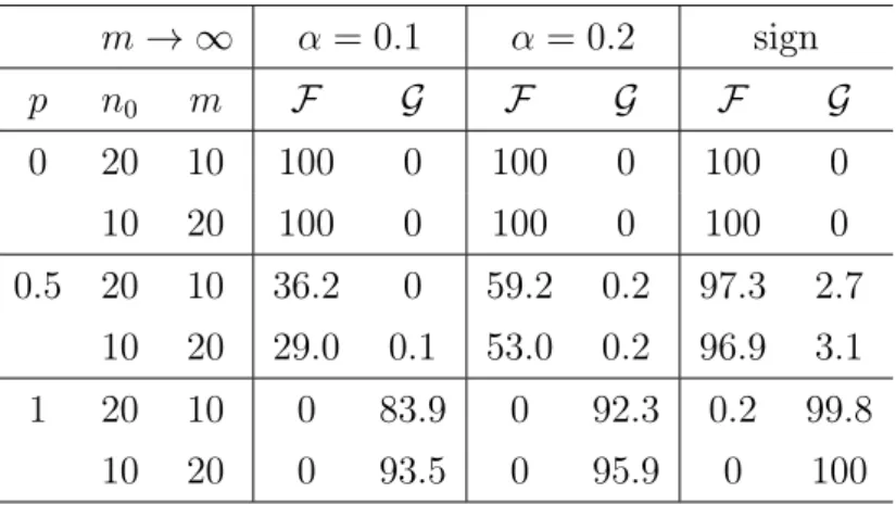
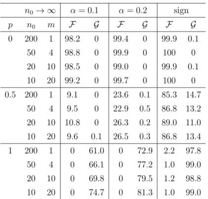
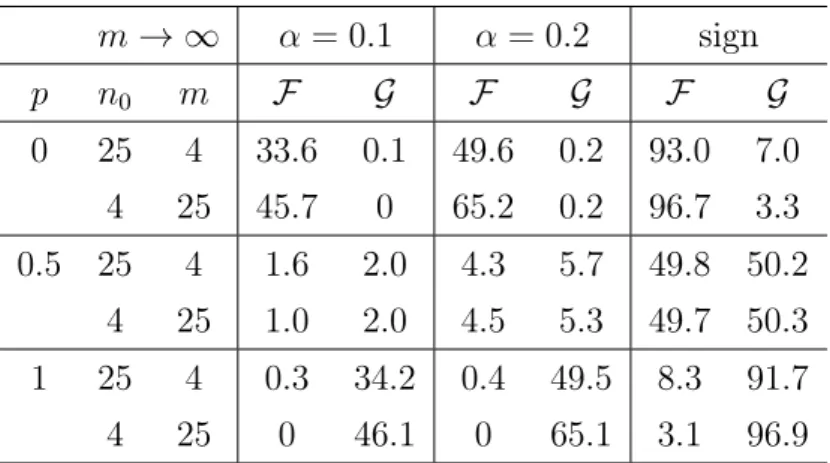
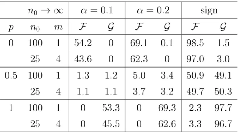
In Chapter 5 simulation studies are carried out to show the performance of the test procedure with moderate sample size.
At the end of this thesis, the extension possibilities of the proposed tests will be discussed in a conclusion in Chapter 6. Some auxiliary lemmas are postponed to the Appendix A.
1.2
Notations
In this section, we introduce some notations which will be used through out this thesis.
For a, b∈R, x= (x1, ..., xd)T, y= (y1, ..., yd)T ∈Rd with d∈N, denote
⌈a⌉:= max{k :k≤a, k ∈Z}, a∧b:= max(a, b), a·N:={a·k :k ∈N}, |x|:= (|x1|, ...,|xd|)T, x+y:= (x1+y1, ..., xd+yd)T, a·x:= (a·x1, ..., a·xd)T,
further we write x≤y if xi ≤yi holds for all i∈ {1, ..., d}and the indicator
I(x≤y) :=
(
1, x≤y,
0, otherwise.
For real valued vectors and matrices k · kdenotes the maximum norm. For any i∈ {1, ..., n}, define the indicator functionδi : [0,1]d→ {0,1} with
δi(z) :=I(zi =z).
For any function ψ : Θ→R, let
˙
ψ := ∂ψ/∂θ1, ..., ∂ψ/∂θp
T
be the column vector of the first partial derivatives of ψ with respect to θ. Further let ψ¨ denote the matrix of the second partial derivatives of ψ with respect to θ.
For a sequence of real valued random variables (Xn)n∈N defined on a
prob-ability space (Ω,F, P), we write
Xn d
−
→ N(µ, σ2),
ifXnconverges to some normally distributed random variable with expectation
µand variance σ2 in distribution, as n→ ∞. Further, we write
Xn −−→a.s. X,
if Xn converges to the random variable X almost surely, as n → ∞.
For the sequences of constants (an)n∈N, nonzero constants (bn)n∈N and real
0, the notation an = O(bn) means that the sequence (an/bn)n∈N is bounded.
Further, Xn = op(bn) means that the sequence of values Xn/bn converges to
zero in probability as n → ∞. The notation Xn = Op(bn) means that the
sequence of values (Xn/bn)n∈N is stochastically bounded, i.e. for any ε > 0,
there exists a finite M >0 such that for eventual all n∈N P(|Xn/bn|> M)< ε.
The right endpoint of a distribution function F is defined as
τF := inf{x:F(x) = 1} ∈(−∞,+∞].
To simplify the notation, we will use a generic constant C > 0 in the proofs, i.e., the value of C might be different in each term containing C. Further, we assume that the notations defined in the proof of a lemma or theorem is only valid within that particular proof.
1.3
Maximum Likelihood Theory
Let X1, ..., Xn be real valued i.i.d. random variables with n ∈ N, their
dis-tribution function H can be estimated by the empirical distribution function
Hn(x) := 1 n n X i=1 I(Xi ≤x), (1.3.1)
for x ∈ R. The properties of the function Hn are well investigated, see for
example Van der Vaart (1998). We list here some of them. First, for each
x∈R
Hn(x) a.s.
−−→H(x).
A stronger result, called the Glivenko-Cantelli theorem, states that the con-vergence holds uniformly over x, i.e.
sup x∈R Hn(x)−H(x) a.s. −−→ 0.
Further, the central limit theorem states the pointwise asymptotic normality:
√ n· Hn(x)−H(x) d − → N 0, H(x) 1−H(x) ,
forx∈R. These convergence properties ofHncan be extended to the so-called empirical integrals: Z ψ(x)dHn(x) = 1 n n X i=1 ψ(Xi),
where ψ :R→Ris a given function. Notice that for any x∈R, Hn(x) =
Z
I(u≤x)dHn(u).
Hence, the empirical integral is a generalization of the empirical distribution function. If R
|ψ(x)|dH(x)<∞, the strong law of large numbers yields
Z ψ(x)dHn(x) a.s. −−→ Z ψ(x)dH(x). While under R
ψ2(x)dH(x)<∞, the central limit theorem gives
√ n· Z ψ(x)dHn(x)− Z ψ(x)dH(x)−→ Nd (0, σ2), where σ2 = Z ψ2(x)dH(x)− Z ψ(x)dH(x)2.
Another possibility to approximate the distribution function H is to use some parametric distribution model classes. For instance, if the random vari-ables X1, ..., Xn represent some kind of lifetimes, the model class is often
as-sumed to be exponential, Weibull or log-normal. Denote the distribution model class by
{F(·|θ) :θ ∈Θ⊂Rp, p∈N}.
Suppose the function F(·|θ) has the density function f(·|θ) for all θ ∈ Θ, an estimate for the parameter is the maximum likelihood estimator, which is defined as ˆ θn := argmax θ∈Θ 1 n n X i=1 logf(Xi|θ).
For any function ψ : R×Θ → R with (x, θ) 7→ ψ(x, θ), we refer to it as
dominated by an H integrable function, if there exists a functionM :R→R,
such that |ψ(x, θ)| ≤M(x) for all (x, θ)∈R×Θ and
Z
M(x)dH(x)<∞.
For the consistency and asymptotic normality of the maximum likelihood estimator, we make the following assumptions.
A1 The density f(·|θ)is strictly positive H-a.s. for all θ ∈Θ.
A2 The set Θis compact and the function logf is twice continuously differ-entiable on Θ.
A3 The functions logf and k∂2logf /∂θ2k are dominated by H integrable
functions. A4 The functionR
logf(x|·)dH(x)has a unique maximum onΘatθ∗, where
θ∗ is an interior point of Θ.
A5 The function k∂logf /∂θk2 is dominated by an H integrable function
and the Hessian matrix
Z
∂2logf(x|θ∗)/∂θ2dH(x) is invertible.
It follows from White (1982) that if A1–A5 hold, then
ˆ
θn a.s.
−−→θ∗
and √n ·(ˆθn−θ∗) convergences to a multi-dimensional normal distribution. The vector θ∗ is called pseudo-true value for the parametric model class. In the case that there exists aθ0, such thatH(·) =F(·|θ0), it holds θ∗ =θ0.
1.4
Censored Data
It is well-known that in practical studies the observation of the survival of a patient is subject to right censoring. Classical example of this type of censoring is that the patient died from other causes than those under study or the patient is still alive by the time of the end of the study.
Let X1, ..., Xn be positive real valued i.i.d. random variables with
distribu-tion funcdistribu-tion H representing the lifetime time of an individual. LetC1, ..., Cn
be real valued i.i.d. random variables with distribution functionJ representing the random censoring times. The observable random variables are
for i ∈ {1, ..., n}. The 0 −1 valued variable ∆i indicates whether Yi is a
censored time (∆i = 0) or not (∆i = 1). Denote the distribution function of
Yi by B. We assume that X1, ..., Xn and C1, ..., Cn are independent, thus for
x∈R
B(x) = 1− 1−H(x)
1−J(x)
.
The distribution function H can be estimated by Kaplan-Meier product-limit estimate (1958): HnKM(x) := 1− Y Y(i)≤x 1− ∆(i) n−i+ 1 ,
where Y(1) ≤ ... ≤ Y(n) are the ordered Y1, ..., Yn, and ∆(1), ...,∆(n) are the
corresponding indicators toY(1), ..., Y(n). Note that the Kaplan-Meier estimator
is a step function and has jumps only at the uncensored observations. Further, in the case of no censoring, it reduces to the empirical distribution function.
The convergence properties of the Kaplan-Meier estimator have been inves-tigated in many papers. Földes and Rejto (1981) showed the strong uniform consistency of the Kaplan-Meier estimator. Lo and Singh (1986) obtained an asymptotic representation, which decomposes HKM
n (x)−H(x) in an average
of i.i.d. terms and a remainder term converging to zero in probability. Based on that representation the asymptotic normality was derived.
In terms of the so-called Kaplan-Meier integrals: R
ψ(x)dHKM
n (x) for a
given function ψ : R → R, Gill (1983) proved its convergence in distribution
under the condition that ψ is a non-negative, continuous and nonincreasing function. Under the same conditions for ψ, Schick et al.(1988) obtained a representation of R
ψ(x)dHnKM(x) as a sum of i.i.d. random variables plus a
remainder. Both of their methods are based on integration by parts. Under some regularity conditions on H, Yang (1994) and Akritas (2000) extended the convergence of R
ψ(x)dHKM
n (x), to those functions ψ satisfying
Z τB
0
ψ2(x)
1−J(x)dH(x)<∞.
In a more general setting, Stute and Wang (1993) pointed out that we can write HnKM(x) = n X i=1 Win·I(Xi ≤x),
where Win := ∆(i) n−i+ 1 n−1 Y j=1 1− ∆(j) n−j+ 1 .
Based on this expression, they showed that under the conditionRτB
0 |ψ(x)|dH(x)< ∞, it holds Z ψ(x)dHnKM(x)−−→a.s. Z τB 0 ψ(x)dH(x).
The asymptotic normality was shown by Stute (1995): if
Z τB 0 ψ2(x) 1−J(x)dH(x)<∞ and Z τB 0 ψ(x, z)C1/2(x)dH(x)<∞, where C(x) := Z x− 0 1 1−B(u) 1−J(u)dJ(u) := Z I(u < x) 1−B(u) 1−J(u)dJ(u), then √ n· Z ψ(x)dHnKM(x)− Z τB 0 ψ(x)dH(x) → N−d (0, σ21), where σ2 1 = Z τB 0 ψ2(x) 1−J(x)dH(x)− Z τB 0 ψ(x)dH(x)2 − Z τB 0 Z τB x ψ(u)dH(u)2· 1−H(x) 1−B(x)2dJ(x).
Note that in the case without censoring (J(x) = 0, for all x),σ2
1 reduces to σ2
as defined in Section 1.3. These results will be applied and extended to the case with covariates in this thesis.
1.5
Kernel Estimate for Conditional
Distribu-tion FuncDistribu-tion
Given the data (X1, z1), ...,(Xn, zn) ∈ R ×[0,1]d with n ∈ N as defined in
Section 1.1. Suppose the distribution functionH(·|z)does not change too fast with respect to z, then the distribution ofXi and Xj should be close if zi and
zj are close. This motivates the construction of estimation of H(·|z) for a z
For each i∈ {1, ..., n}, denote the weight function wni :Rd×R+ →R+ by wni(z, h) := K(zi−z h ) Pn k=1K( zk−z h ) ,
where the function K : Rd → R+ is called kernel function and h > 0
band-width. The Nadaraya-Watson kernel estimate (Nadaraya (1964), Watson (1964)) is defined by ˆ Hn(x|z) := n X i=1 wni(z, h)·I(Xi ≤x). (1.5.1)
The bandwidth h controls the smoothness of the estimate. Common choices for K are, for instance, uniform and Epanechnikov kernel, which are defined by K(x) :=1 2·I(|x| ≤1) and K(x) := 3 4(1−x 2)·I(|x| ≤1), respectively.
Another possibility to choose weights is the so called Gasser-Müller weights (Gasser and Müller (1984)). In our setting, if z is one dimensional (d= 1) and
m= 1, the weights of the Gasser-Müller weights are defined by
wni(z, h) := Z zi zi−1 1 hK z−u h du, with z0 = 0.
The convergence properties of the kernel estimator for distribution function were shown in for example Aerts et al.(1994), Györfi et al.(2002) and Li and Racine (2007). The main conditions for the asymptotic properties are: first, the distribution function H is differentiable with respect to z, so H(·|z) does not change too fast in z and can be estimated with data at zi close to z.
Secondly, n0h → ∞ and h → 0 as n0 → ∞, i.e. the number of data in any
fixed small interval tends to infinity.
In the case with censoring, for each i ∈ {1, ..., n} we denote the right cen-soring random variable at zi as Ci with distribution function J(·|zi). Further
denote
Yi := min(Xi, Ci) and ∆i :=I(Xi ≤Ci).
Beran (1981) introduced a kernel estimator for the conditional distribution. His estimator is a generalization of the Kaplan-Meier estimator and is
some-times called conditional Kaplan-Meier estimator: ˆ HnKM(x|z) := 1− Y Y(i)≤x 1− wn(i)(z, h)·∆(i) 1−Pi−1 j=1wn(j)(z, h) .
Here Y(1) ≤ ... ≤ Y(n) denote the ordered Y1, ..., Yn, while ∆(1), ...,∆(n) and
wn(1)(z, h), ..., wn(n)(z, h)represent the corresponding indicators and weights of
Y(1), ..., Y(n), respectively. Note that in the case without censoring HˆnKM(x|z)
reduces to the kernel estimator Hˆn(x|z) defined in (1.5.1).
The uniform consistency and asymptotic normality of Beran’s estimator was studied by Dabrowska (1987, 1989), Mckeague and Utikal (1990), Akritas (1994) and González and Cadarso (1994) in the random design case, where the covariatez is also assumed to be a random variable. It was extend to the case with discrete covariates by Du and Akritas (2002). The fixed design case was investigated by Van Keilegom and Veraverbeke (1996, 1997a, 1997b) using Gasser-Müller weights.
Model Selection Testing
In this chapter, we assume that the observations (X1, z1),..., (Xn, zn) and the
distribution functionH(·|z)are defined as in Section 1.1. Given two parametric distribution model classes:
F :={F(·|θ, z) :θ ∈Θ⊂Rp, z ∈[0,1]d}
and
G:={G(·|γ, z) :γ ∈Γ⊂Rq, z ∈[0,1]d},
where Θ and Γ are compact intervals and the constant d, p, q ∈ N, we will
construct model selection tests to answer the question which of the two model classes approximates the underlying family of distributions better. The dis-tances of the model classes and the underlying distributions will be defined based on the Cramér von-Mises distances, which is often used in the goodness-of-fit test. The test statistics are defined as the difference of the estimated distances. Asymptotic normality of the test statistics will be proven. Based on this asymptotic behavior decision rules for the tests will be formulated.
This chapter is organized as follows: in Section 2.1, some notations and the hypotheses of the model selection tests for this chapter will be introduced. Section 2.2 deals with the case that n0 is fixed and m → ∞, i.e. the number
of covariates values is fixed and the number of observations at each covariates values tends to infinity. The underlying distribution function H will be esti-mated by the empirical distribution at each covariates value. In Section 2.3, it is assumed that m is fixed and n0 → ∞. The empirical distribution function
is replaced by the kernel Nadaraya-Watson estimator as defined in Section 1.5. 13
For simplicity of notation, we assume that the notations defined in Section 2.1 are valid through out this chapter and the notations defined in Section 2.2 and Section 2.3 are only valid in that particular section.
2.1
Notations and Hypotheses
In this section, we will introduce a distance measure between the underlying distribution and the given model classes based on the likelihood theory. First, we define the joint distribution function by Q:R×[0,1]d →[0,1] with
Q(x, z) :=
Z Z
I(u≤x)·I(v ≤z)dH(u|v)dv,
where the inner integration is with respect to the variable u. The empirical distribution function at covariate z and the joint empirical distribution are then given by Hn, Qn:R×[0,1]d →[0,1] with
Hn(x|z) := 1 m n X i=1 δi(z)·I(Xi ≤x), where δi(z) := I(zi =z)and Qn(x, z) := 1 n n X i=1 I(Xi ≤x)·I(zi ≤z) = 1 n0 n0 X i=1 Hn(x|zi)·I(zi ≤z).
For any functionψ: R×Θ×[0,1]d→R, we get then
Z ψ(x, θ, z)dQ(x, z) = Z Z ψ(x, θ, z)dH(x|z)dz, Z ψ(x, θ, z)dQn(x, z) = 1 n n X i=1 ψ(Xi, θ, zi) = 1 n0 n0 X i=1 Z ψ(x, θ, zi)dHn(x|zi).
Denote the logarithmic likelihood function for the model classF asLˆf,n : Θ→
R with
ˆ
Lf,n(θ) :=
Z
logf(x|θ, z)dQn(x, z),
where for each (θ, z) ∈ Θ×[0,1]d, the function f(·|θ, z) denotes the density
function ofF(·|θ, z). The maximum likelihood estimatorθˆnfor the model class
F is defined as a measurable selection:
ˆ
θn := argmax θ∈Θ
ˆ
By the compactness of the set Θ, the estimator θˆn exists, if for any (x, z) ∈
R× [0,1]d the function f(x|·, z) is continuous in θ. Further, we define the
functions Lf,n0, Lf,∞: Θ→Rand the vectors θn0, θ∗ ∈Θ by
Lf,n0(θ) := 1 n0 n0 X i=1 Z logf(x|θ, zi)dH(x|zi), θn0 := argmax θ∈Θ Lf,n0(θ), Lf,∞(θ) := Z logf(x|θ, z)dQ(x, z), θ∗ := argmax θ∈Θ Lf,∞(θ).
We will show in the next two sections that under some regularity conditions the following relations hold:
ˆ Lf,n m→∞ −−−→Lf,n0 n0→∞ց ւn0→∞ Lf,∞. And we have then
ˆ θn m→∞ −−−→θn0 n0→∞ց ւn0→∞ θ∗.
We define the distance dH(F) between the underlying family of distribution
functions H and the model classF as
1 n0 n0 X i=1 Z H(x|zi)−F(x|θn0, zi) 2 dH(x|zi), (2.1.1)
for the case with n0 fixed andm → ∞and
Z
H(x|z)−F(x|θ∗, z)
2
dQ(x, z) (2.1.2) for the case with m fixed and n0 → ∞, respectively.
Letg,γˆn,γn0,γ∗ and dH(G)denote the counterparts for the model class G.
We will propose model selection tests of the null hypothesis
meaning that the two models are equally close to H, against
HF : dH(F)< dH(G)
meaning H is closer to F than toG or
HG : dH(F)> dH(G)
meaning H is closer to G than toF.
We call a function ψ : R×Θ×[0,1]d→ R with (x, θ, z)7→ ψ(x, θ, z) asH
integrable or H square integrable, if for each (θ, z)∈Θ×[0,1]d,
Z
ψ(x, θ, z)dH(x|z)<∞ or
Z
ψ2(x, θ, z)dH(x|z)<∞
holds.
We refer the function ψ as dominated by anH integrable function, if there exists an H integrable function M : R×[0,1]d → R, such that |ψ(x, θ, z)| ≤ M(x, z)for all (x, θ, z)∈R×Θ×[0,1]d.
If there exists a function M : R → R such that for all (x, θ, z) ∈ R×Θ×
[0,1]d, ψ(x, θ, z) < M(x) and Z M(x)dx <∞.
we call ψ dominated by a Lebesgue integrable function independent ofz. If there exists a function M : R → R such that for all (x, θ, z) ∈ R×Θ×
[0,1]d, ψ(x, θ, z) < M(x) and Z M(x)dH(x|z)<∞,
we refer ψ as dominated by an H integrable function independent of z. Further the domination by an H square integrable function (independent of z) is defined analogously.
In Section 2.2, we assume all the convergences are taken by lettingm → ∞. In Section 2.3, we assume all the convergences are taken by letting n0 → ∞.
Note that since n = m·n0, in Section 2.2, n ∈ n0 ·N :={n0·a : a ∈ N}, in
2.2
The Case with Number of Observations at
Each Covariate Tending to Infinity
In this section, the distance dH(F) defined in (2.1.1) is estimated by
ˆ dH,n(F) := Z Hn(x|z)−F(x|θˆn, z) 2 dQn(x, z).
For the class G, the estimator dˆH,n(G)is defined in an analogous way. As test
statistic we take the difference of the estimated distances
Tn := ˆdH,n(F)−dˆH,n(G).
The main results of this section is the asymptotic normality of √n·Tn and
the determination of a consistent estimator for the asymptotic variance of
√
n ·Tn. Based on these results, decision rules for the model selection test
will be formulated. In this section we make the following assumptions. They are stated in terms of the model class F, it is understood that corresponding assumptions are also made for the model class G.
B1 For each (θ, z) ∈ Θ×[0,1]d, the density function f(·|θ, z) : R → R is
strictly positive H(·|z)-a.s.
B2 The function logf is three times continuously differentiable inθ on Θ. B3 The function logf is dominated by an H integrable function.
B4 The function Lf,n0 has a unique maximum on Θ at θn0, which is an
interior point of Θ.
B5 The functionsk∂logf /∂θkandk∂2logf /∂θ2kare dominated byHsquare
integrable functions. The Hessian matrix L¨f,n0(θn0)is invertible with
in-verse L¨−f,n10(θn0).
B6 For any i, j, k ∈ {1,2, ..., p}, the function ∂3logf /∂θ
i∂θj∂θk is
domi-nated by an H integrable function.
These assumptions are regular assumptions in the framework of the maxi-mum likelihood theory. The asymptotic properties of θˆn, which we will show
in this section, can be reached also under weaker conditions. However, the fo-cus of this thesis is model selection test, therefore we use the more restrictive conditions to avoid technical difficulties.
Lemma 2.2.1. Define the functionψ :R×[0,1]d→R. Ifψ is an H integrable
function, then Z ψ(x, z)dQn(x, z)− 1 n0 n0 X i=1 Z ψ(x, zi)dH(x|zi) a.s. −−→0. (2.2.1)
If ψ is an H square integrable function, then
√ n· Z ψ(x, z)dQn(x, z)− 1 n0 n0 X i=1 Z ψ(x, zi)dH(x|zi) d − → N(0, σ2), (2.2.2) where σ2 = 1 n0 n0 X i=1 Z ψ2(x, zi)dH(x|zi)− Z ψ(x, zi)dH(x|zi) 2 .
Proof. We denote first for each i∈ {1, ..., m},
Ui := 1 n0 n0 X j=1 ψ(X(i−1)·n0+j, z(i−1)·n0+j).
Note that U1, ..., Um are i.i.d. and we can write
Z ψ(x, z)dQn(x, z) = 1 m m X i=1 Ui.
Further, the expectation
E Z ψ(x, z)dQn(x, z) = 1 n0 n0 X i=1 Z ψ(x, zi)dH(x|zi)
and by independence of X1, ..., Xn the variance
V ar√ n· Z ψ(x, z)dQn(x, z) = 1 n n X i=1 V ar ψ(Xi, zi) =σ2.
Therefore, the assertions follow from the strong law of large numbers and central limit theorem for i.i.d data.
Based on Lemma 2.2.1, we will show in the next two lemmas the consistency of the maximum likelihood estimator θˆn to θn0 and the asymptotic properties
of √n·(ˆθn−θn0), respectively.
Lemma 2.2.2. If B1–B5 hold, then kθˆn−θn0k →0 a.s.
Proof. Under B1–B3 the functionsLˆf,n andLf,n0 are continuous onΘ. Under
B4 the pseudo true value θn0 is unique and is a well separated maximizer of
the function Lf,n0. If we can show
sup θ∈Θ Lˆf,n(θ)−Lf,n0(θ) →0 a.s.,
then the assertion follows from an argmax theorem, see for example Theorem 2.12 in Kosorok (2008). Under B5, for each z ∈[0,1]d, there exists a function
M(·, z) :R→R and a constantC > 0, such that
sup θ∈Θk ∂logf(x|θ, z)/∂θk ≤M(x, z) and 1 n0 n0 X i=1 Z M(x, zi)dH(x|zi)< C. By Lemma 2.2.1 with ψ(x, z) =M(x, z), Z M(x, z)dQn(x, z) a.s. −−→ n1 0 n0 X i=1 Z M(x, zi)dH(x|zi).
Hence, for eventually all n ∈n0·N
sup θ∈Θ Z ∂logf(x|θ, z) ∂θ dQn(x, z)≤ Z M(x, z)dQn(x, z)< C a.s. (2.2.3)
Since Θ is compact, for any constant ε > 0 and the constant C above, there exist compact non-empty subsetsSl,1, ..., Sl,l ⊆Θwith l ∈N such that
Θ⊆ l [ k=1 Sl,k and sup θ,θ˜∈Sl,k kθ−θ˜k ≤ ε 3Cp. (2.2.4)
By the compactness of the sets Sl,k there exist vectors θnl,k, θl,k ∈ Sl,k, such
that sup θ∈Sl,k ˆ Lf,n(θ) = ˆLf,n(θnl,k) and inf θ∈Sl,k Lf,n0(θ) =Lf,n0(θl,k).
For a fixed point θ˙l,k ∈Sl,k, by the triangle inequality, we get sup θ∈Sl,k ˆ Lf,n(θ)− inf θ∈Sl,k Lf,n0(θ) ≤ Lˆf,n(θnl,k)−Lˆf,n( ˙θl,k) + Lˆf,n( ˙θl,k)−Lf,n0( ˙θl,k) + Lf,n0( ˙θl,k)−Lf,n0(θl,k) . (2.2.5)
By a Taylor expansion with an intermediate point θ˜nl,k between θnl,k and θ˙l,k,
the first term on the right-hand side in (2.2.5) can be written as
Lˆf,n(θnl,k)−Lˆf,n( ˙θl,k) = Z ∂logf(x|θ˜nl,k, z) ∂θ dQn(x, z) T ·(θnl,k−θ˙l,k) .
By (2.2.3) and (2.2.4), for eventually all n ∈ n0·N, the right term of the last
equation is bounded almost surely by
p· sup θ,θ˜∈Sl,k kθ−θ˜k · Z ∂logf(x|θ˜nl,k, z) ∂θ dQn(x, z)≤p· ε 3Cp·C = ε 3.
Analogously, for the third term on the right-hand side in (2.2.5), we have the same result. For the second term on the right-hand side in (2.2.5) by Lemma 2.2.1 with ψ(x, z) = logf(x|θ˙l,k, z) under B3, forn large enough we have
Lˆf,n( ˙θl,k)−Lf,n0( ˙θl,k) < ε 3 a.s.
Hence, there exists an Nl,k, such that for all n > Nl,k,
sup θ∈Sl,k ˆ Lf,n(θ)− inf θ∈Sl,k Lf,n0(θ) < ε a.s.
Analogously, there exists an N′
l,k ∈N, such that for alln > Nl,k′ ,
inf θ∈Sl,k ˆ Lf,n(θ)− sup θ∈Sl,k Lf,n0(θ) < ε a.s.
Hence, for all n >max1≤k≤l{Nl,k, Nl,k′ },
sup θ∈Θ Lˆf,n(θ)−Lf,n0(θ) ≤max k θsup∈Sl,k Lˆf,n(θ)−Lf,n0(θ) ≤max k n sup θ∈Sl,k ˆ Lf,n(θ)− inf θ∈Sl,k Lf,n0(θ) , inf θ∈Sl,k ˆ Lf,n(θ)− sup θ∈Sl,k Lf,n0(θ) o < ε a.s.
Lemma 2.2.3. If B1–B6 hold, then
√ n· kθˆn−θn0k=Op(1), √ n· θˆn−θn0 + ¨L−f,n1 0(θn0)·L˙ˆf,n(θn0) =op(1).
Proof. By a Taylor expansion, there exists a θ˜n lying betweenθn0 andθˆn such
that
˙ˆ
Lf,n(ˆθn) = L˙ˆf,n(θn0) +L¨ˆf,n(˜θn)·(ˆθn−θn0).
By the definition of θˆn it follows that
L˙ˆf,n(θn0) +L¨ˆf,n(˜θn)·(ˆθn−θn0)
= 0. (2.2.6)
Under B5 and by Lemma 2.2.1 with ψ(x, z) = ∂logf(x|θn0, z)/∂θj, for j ∈
{1, ..., p}, we have √ n· Z ∂logf(x|θn0, z) ∂θj dQn(x, z)− 1 n0 n0 X i=1 Z ∂logf(x|θn0, zi) ∂θj dH(x|zi)
converges in distribution to a normal distribution. Further by the definition of θn0, for each j ∈ {1, ..., p}, under B4 and B5,
1 n0 n0 X i=1 Z ∂logf(x |θn0, zi) ∂θj dH(x|zi) = 0. (2.2.7) Hence, √ n· L˙ˆf,n(θn0) = sup j∈{1,...,p} √ n· Z ∂logf(x |θn0, z) ∂θj dQn(x, z) =Op(1). (2.2.8) Under B3 and B5 we can switch the order of integration and differentiation in the Hessian matrix ofLf,n0(θn0), i.e.
¨ Lf,n0(θn0) = 1 n0 n0 X i=1 Z ∂2logf(x |θn0, zi) ∂θ2 dH(x|zi).
By a Taylor expansion, there exists a θ¯n lying between θ˜n and θn0 such that
L¨ˆf,n(˜θn)−L¨f,n0(θn0) ≤ L¨ˆf,n(˜θn)−L¨ˆf,n(θn0) + L¨ˆf,n(θn0)−L¨f,n0(θn0) ≤p·max i,j,k Z ∂3logf(x|θ¯ n, z) ∂θi∂θj∂θk dQn(x, z) k ˜ θn−θn0k + max i,j Z ∂2logf(x|θ n0, z) ∂θi∂θj dQn(x, z)− 1 n0 n0 X i=1 Z ∂2logf(x|θ n0, zi) ∂θi∂θj dH(x|zi) . (2.2.9) Under B1–B6, by Lemma 2.2.2, the first term on the right side of (2.2.9) tends to zero. Further, for eachi,j ∈ {1, ..., p}by Lemma 2.2.1 withψ(x, z) =
∂2logf(x|θ
n0, z)/∂θi∂θjunder B5 the second term tends to zero as well.
There-fore,
kL¨ˆf,n(˜θn)−L¨f,n0(θn0)k →0 a.s.
Since the matrix L¨f,n0(θn0) is invertible under B5, by the continuity of the
determinant function the matrix L¨ˆf,n(˜θn) is also invertible for eventually all
n ∈n0·N. Further, by the continuity of the inversion operator we obtain
kL¨ˆ−f,n1(˜θn)−L¨f,n−10(θn0)k →0 a.s. (2.2.10)
as well. It follows then from (2.2.6), (2.2.8) and (2.2.10) that
√ n· θˆn−θn0 + ¨L−f,n1 0(θn0)·L˙ˆf,n(θn0) =√n· θˆn−θn0 +L¨ˆ−f,n1(˜θn)·L˙ˆf,n(θn0)− L¨ˆf,n−1(˜θn)−L¨−f,n1 0(θn0) ·L˙ˆf,n(θn0) ≤p· L¨ˆ−f,n1(˜θn)−L¨−f,n1 0(θn0) · √ n·L˙ˆf,n(θn0) =op(1).
By the boundedness of L¨−f,n10(θn0)and (2.2.8) we get
√ n· kθˆn−θn0k ≤ √ n· kθˆn−θn0 + ¨L −1 f,n0(θn0)·L˙ˆf,n(θn0)k +p· kL¨−f,n10(θn0)k · √ n· kL˙ˆf,n(θn0)k=Op(1).
In order to state the main theorems we introduce the functions CF : Θ →
Rp, NF :R×Θ×[0,1]d →Rand a constant σ2 F with CF(θ) := 1 n0 n0 X i=1 Z H(x|zi)−F(x|θ, zi) ·F˙(x|θ, zi)dH(x|zi), NF(x, θ, z) := H(x|z)−F(x|θ, z) 2 + 2 Z ∞ x H(u|z)−F(u|θ, z) dH(u|z) + 2CFT(θn0)·L¨ −1 f,n0(θn0)· ∂logf(x|θ, z) ∂θ , σF2 := 1 n0 n0 X i=1 Z NF2(x, θn0, zi)dH(x|zi)− Z NF(x, θn0, zi)dH(x|zi) 2 .
Under B5 and B7, the functions CF and NF exist, the constant σ2F <∞. In the next theorem we show the asymptotic normality of the estimated distance.
Theorem 2.2.4. Let B1–B7 be satisfied, then
√
n· dˆH,n(F)−dH(F)
d
−
Proof. Note that for(x, z)∈R×[0,1]d,Hn(x|z)−F(x|θˆn, z)can be represented as Hn(x|z)−H(x|z)+ H(x|z)−F(x|θn0, z) − F(x|θˆn, z)−F(x|θn0, z) .
Hence, we can write
√ n·dˆH,n(F) = √ n· Z Hn(x|z)−H(x|z) 2 dQn(x, z) + 2√n· Z Hn(x|z)−H(x|z) · H(x|z)−F(x|θn0, z) dQn(x, z) −2√n· Z H(x|z)−F(x|θn0, z) · F(x|θˆn, z)−F(x|θn0, z) dQn(x, z) +√n· Z H(x|z)−F(x|θn0, z) 2 dQn(x, z) −2√n· Z Hn(x|z)−H(x|z) · F(x|θˆn, z)−F(x|θn0, z) dQn(x, z) +√n· Z F(x|θˆn, z)−F(x|θn0, z) 2 dQn(x, z) =: 6 X k=1 Tkn. For T1n we have T1n=√n· Z Hn2(x|z)−2H(x|z)Hn(x|z) +H2(x|z) dQn(x, z) =√n· 1 n0 n0 X i=1 Z Hn2(x|zi)dHn(x|zi)−2√n· 1 n0 n0 X i=1 Z H(x|zi)Hn(x|zi)dHn(x|zi) +√n· Z H2(x|z)dQn(x, z) =√n· 1 n0 n0 X i=1 Z Z Z I(u≤x)I(t≤x)dHn(u|zi)dHn(t|zi)dHn(x|zi) −2√n· 1 n0 n0 X i=1 Z Z I(u≤x)H(x|zi)dHn(u|zi)dHn(x|zi) +√n· Z H2(x|z)dQ n(x, z). (2.2.11)
By Lemma A.1.1 with k= 3,Xij =Xj fori∈ {1,2,3}, j ∈ {1, ..., n} and
ψ(u, t, x, z) = I(u≤x)I(t ≤x),
since
for anyi1, i2, i3 ∈ {1, ..., n}, thus the first term on the right-hand side of (2.2.11) can be written as √ n· 1 n0 n0 X i=1 Z Z Z I(u≤x)I(t≤x)dHn(u|zi)dH(t|zi)dH(x|zi) +√n· 1 n0 n0 X i=1 Z Z Z I(u≤x)I(t ≤x)dH(u|zi)dHn(t|zi)dH(x|zi) +√n· 1 n0 n0 X i=1 Z Z Z I(u≤x)I(t ≤x)dH(u|zi)dH(t|zi)dHn(x|zi) −2√n· 1 n0 n0 X i=1 Z Z Z I(u≤x)I(t ≤x)dH(u|zi)dH(t|zi)dH(x|zi) +op(1) =2√n· 1 n0 n0 X i=1 Z H(x|zi)Hn(x|zi)dH(x|zi) +√n· 1 n0 n0 X i=1 Z H2(x|zi)dHn(x|zi) −2√n· 1 n0 n0 X i=1 Z H2(x|zi)dH(x|zi) +op(1).
Analogously, by Lemma A.1.1 with k = 2, Xij = Xj for i ∈ {1,2}, j ∈
{1, ..., n}and ψ(u, x, z) =I(u≤x)H(x|z), since E[ψ2(Xi1, Xi2, z)] =E[I(Xi1 ≤Xi2)H 2(X i2|z)]≤1
for any i1, i2 ∈ {1, ..., n}, hence the second term on the right-hand side of
(2.2.11) can be written as −2√n· 1 n0 n0 X i=1 Z Z I(u≤x)H(x|zi)dHn(u|zi)dH(x|zi) −2√n· 1 n0 n0 X i=1 Z Z I(u≤x)H(x|zi)dH(u|zi)dHn(x|zi) + 2√n· 1 n0 n0 X i=1 Z Z I(u≤x)H(x|zi)dH(u|zi)dH(x|zi) +op(1) =−2√n· 1 n0 n0 X i=1 Z H(x|zi)Hn(x|zi)dH(x|zi)−2√n· 1 n0 n0 X i=1 Z H2(x|zi)dHn(x|zi) + 2√n· 1 n0 n0 X i=1 Z H2(x|zi)dH(x|zi) +op(1).
Hence, we get T1n=2 √ n· 1 n0 n0 X i=1 Z H(x|zi)Hn(x|zi)dH(x|zi) +√n· 1 n0 n0 X i=1 Z H2(x|zi)dHn(x|zi)−2 √ n· 1 n0 n0 X i=1 Z H2(x|zi)dH(x|zi) −2√n· 1 n0 n0 X i=1 Z H(x|zi)Hn(x|zi)dH(x|zi)−2√n· 1 n0 n0 X i=1 Z H2(x|zi)dHn(x|zi) + 2√n· 1 n0 n0 X i=1 Z H2(x|zi)dH(x|zi) +√n· Z H2(x|z)dQn(x, z) +op(1) = op(1). (2.2.12)
With the same arguments, it can be shown that
T2n=2√n· Z Z ∞ x H(u|z)−F(u|θn0, z) dH(u|z)dQn(x, z) −2√n· 1 n0 n0 X i=1 Z Z ∞ x H(u|zi)−F(u|θn0, zi) dH(u|zi)dH(x|zi) +op(1).
By a Taylor expansion, there exists a θ˜n between θˆn and θn0, such that
T3n=−2√n· Z H(x|z)−F(x|θn0, z) ·F˙(x|θn0, z)dQn(x, z) T ·(ˆθn−θn0 −2√n·(ˆθn−θn0 T · Z H(x|z)−F(x|θn0, z) ·F¨(x|θ˜n, z)dQn(x, z)·(ˆθn−θn0 .
For the first term on the right-hand side of the last equation, under B7, each component of the vector H(x|z)−F(x|θn0, z)
·F˙(x|θn0, z) is H integrable,
hence, by Lemma 2.2.1 we get
Z H(x|z)−F(x|θn0, z) ·F˙(x|θn0, z)dQn(x, z)−CF(θn0) =op(1).
For the second term note that under B7,
Z H(x|z)−F(x|θn0, z) ·F¨(x|θ˜n, z)dQn(x, z)
is stochastically bounded. Hence, by Lemma 2.2.3 under B1–B6, the second term on the right-hand side is equal to op(1) and
T3n=−2√n·CFT(θn0)·(ˆθn−θn0
+op(1) = 2√n·CFT(θn0)·L¨
−1
Analogously, we can show that T5n= 2√n· Z Hn(x|z)−H(x|z) ·F˙(x|θn0, z)dQn(x, z) T ·(ˆθn−θn0) +op(1).
By Cauchy-Schwarz’s inequality, we get
Z Hn(x|z)−H(x|z) ·F˙(x|θn0, z)dQn(x, z) ≤ Z Hn(x|z)−H(x|z) · kF˙(x|θn0, z)kdQn(x, z) ≤ Z Hn(x|z)−H(x|z) 2 dQn(x, z) 1/2 · Z kF˙(x|θn0, z)k 2dQ n(x, z) 1/2 ≤T1n·n−1/2 1/2 · Z kF˙(x|θn0, z)k 2dQ n(x, z) 1/2 =op(1)
where the last step follows from (2.2.12) and B7. Hence, it follows from Lemma 2.2.3 that T5n=op(1).
By the same arguments, there exists a θ¯n between θˆn and θn0, such that
|T6n| ≤√n·p2
Z
kF˙(x|θ¯n, z)k2dQn(x, z)· kθˆn−θn0k
2 =o
p(1).
Therefore, by the definition of the function NF,
√ n·dˆH,n(F) =√n· Z NF(x, θn0, z)dQn(x, z) −2√n· 1 n0 n0 X i=1 Z Z ∞ x H(u|zi)−F(u|θn0, zi) dH(u|zi)dH(x|zi) +op(1).
Note that by the definition of θn0, under B3 and B5,
1 n0 n0 X i=1 Z CFT(θn0)·L¨ −1 f,n0(θn0)· ∂logf(x|θn0, zi) ∂θ dH(x|zi) =CFT(θn0)·L¨ −1 f,n0(θn0)·L˙f,n0(θn0) = 0.
Thus, we can write
dH(F) = 1 n0 n0 X i=1 Z NF(x, θn0, zi)dH(x|zi) −2· 1 n0 n0 X i=1 Z Z ∞ x H(u|zi)−F(u|θn0, zi) dH(u|zi)dH(x|zi). Therefore, we have √ n· dˆH,n(F)−dH(F)
=√n· Z NF(x, θn0, z)dQn(x, z)− 1 n0 n0 X i=1 Z NF(x, θn0, zi)dH(x|zi) +op(1). (2.2.13) Under B5 and B7, the functionNF isHsquare integrable. Hence, the assertion follows from Lemma 2.2.1 with ψ(x, z) = NF(x, θn0, z).
For the estimation of the asymptotic variance σ2
F we define the functions
CF,n : Θ→Rp, and NF,n :R×Θ×[0,1]d→R with CF,n(θ) := Z Hn(x|z)−F(x|θ, z) ˙ F(x|θ, z)dQn(x, z), NF,n(x, θ, z) := Hn(x|z)−F(x|θ, z) 2 + 2 Z ∞ x Hn(u|z)−F(u|θ, z) dHn(u|z) + 2CFT,n(ˆθn)·L¨ˆ−f,n1(ˆθn)· ∂logf(x|θ, z) ∂θ .
In the next lemma, we show that σ2
F can be estimated consistently by
ˆ σF2,n := Z NF2,n(x,θˆn, z)dQn(x, z)− 1 n0 n0 X i=1 Z NF,n(x,θˆn, zi)dHn(x|zi) 2 .
Lemma 2.2.5. If B1–B7 hold, then we have
ˆ
σF2,n =σF2 +op(1).
Proof. First, we show that for each θ ∈Θ,
Z NF2,n(x, θ, z)dQn(x, z)− 1 n0 n0 X i=1 Z NF2(x, θ, zi)dH(x|zi) =op(1). (2.2.14) Note that R Hn(x|z)−F(x|θ, z) 4 dQn(x, z)is a part of Z NF2,n(x, θ, z)dQn(x, z)
and its counterpart in
1 n0 n0 X i=1 Z N2 F(x, θ, zi)dH(x|zi) is 1 n0 n0 X i=1 Z H(x|zi)−F(x|θ, zi) 4 dH(x|zi).
In the sequel, we show that Z Hn(x|z)−F(x|θ, z) 4 dQn(x, z) = 1 n0 n0 X i=1 Z H(x|zi)−F(x|θ, zi) 4 dH(x|zi) +op(1). (2.2.15) Note that Z Hn(x|z)−F(x|θ, z) 4 dQn(x, z) = 1 n0 n0 X i=1 Z Hn4(x|zi)−4Hn3(x|zi)F(x|θ, zi) + 6Hn2(x|zi)F2(x|θ, zi) −4Hn(x|zi)F3(x|θ, zi) +F4(x|θ, zi) dHn(x|zi). (2.2.16)
By Corollary A.1.2, with k = 5 and Xij = Xj for i ∈ {1, ...,5}, j ∈ {1, ..., n}
and ψ(x1, ..., x5, z) = 4 Y j=1 I(xj ≤x5), since E[ψ2(Xi1, ..., Xi5, z)] = E hY4 j=1 I(Xij ≤Xi5) i ≤1, we get 1 n0 n0 X i=1 Z Hn4(x|zi)dHn(x|zi) = 1 n0 n0 X i=1 Z · · · Z 4 Y j=1 I(xj ≤x5)dHn(x1|zi)· · ·dHn(x5|zi) = 1 n0 n0 X i=1 Z · · · Z 4 Y j=1 I(xj ≤x5)dH(x1|zi)· · ·dH(x5|zi) +op(1) = 1 n0 n0 X i=1 Z H4(x|z i)dH(x|zi) +op(1).
With similar arguments, we can show that similar results hold for the other terms on the right-hand side of (2.2.16). Therefore, (2.2.15) holds.
Analogously, it can be shown that
Z Z ∞ x Hn(x|z)−F(x|θ, z) 2 Hn(u|z)−F(u|θ, z) dHn(u|z)dQn(x, z)
= 1 n0 n0 X i=1 Z Z ∞ x H(x|zi)−F(x|θ, zi) 2 H(u|zi)−F(u|θ, zi) dH(u|zi)dH(x|zi) +op(1) (2.2.17) and Z Z ∞ x Hn(u|z)−F(u|θ, z) dHn(u|z) 2 dQn(x, z) =1 n0 n0 X i=1 Z Z ∞ x H(u|zi)−F(u|θ, zi) dH(u|zi) 2 dH(x|zi) +op(1). (2.2.18) For the rest terms of
Z NF2,n(x, θ, z)dQn(x, z) and 1 n0 n0 X i=1 Z NF2(x, θ, zi)dH(x|zi), note that kCT F,n(ˆθn)−CFT(θn0)k ≤ kC T F,n(ˆθn)−CFT,n(θn0)k+kC T F,n(θn0)−C T F(θn0)k.
Under B7, the derivative of CT
F,n is stochastically bounded on Θ. Hence, by
Lemma 2.2.2 under B1-B5
kCFT,n(ˆθn)−CFT,n(θn0)k=op(1).
Further, it follows from Corollary A.1.2 and Lemma 2.2.1 that under B7
kCFT,n(θn0)−C
T
F(θn0)k=op(1).
Therefore,
kCFT,n(ˆθn)−CFT(θn0)k=op(1).
Further, analogously to (2.2.10) under B6, it can be shown that
kL¨ˆ−f,n1(ˆθn)−L¨f,n−10(θn0)k=op(1).
Thus, under B5 Corollary A.1.2 implies
Z Hn(x|z)−F(x|θ, z) 2 ·CFT,n(ˆθn)·L¨ˆ−f,n1(ˆθn)· ∂logf(x|θ, z) ∂θ dQn(x, z) =CFT,n(ˆθn)·L¨−f,n1(ˆθn)· Z Hn(x|z)−F(x|θ, z) 2 ·∂logf(x|θ, z) ∂θ dQn(x, z)
= 1 n0 n0 X i=1 CFT(θn0)·L¨ −1 f,n0(θn0)· Z H(x|zi)−F(x|θ, zi) 2 ·∂logf(x|θ, zi) ∂θ dH(x|zi) +op(1) (2.2.19) With the same arguments, it follows further
Z Z ∞ x Hn(u|z)−F(u|θ, z) dHn(u|z)·CFT,n(ˆθn)·L¨ˆ−f,n1(ˆθn)· ∂logf(x|θ, z) ∂θ dQn(x, z) = 1 n0 n0 X i=1 CFT(θn0)·L¨ −1 f,n0(θn0) × Z Z ∞ x H(u|zi)−F(u|θ, zi) dH(u|zi)· ∂logf(x|θ, zi) ∂θ dH(x|zi) +op(1) (2.2.20) and Z CFT,n(ˆθn)·L¨ˆ−f,n1(ˆθn)· ∂logf(x|θ, z) ∂θ 2 dQn(x, z) = 1 n0 n0 X i=1 Z CFT(θn0)·L¨ −1 f,n0(θn0)· ∂logf(x|θ, zi) ∂θ 2 dH(x|zi) +op(1). (2.2.21)
By (2.2.15)–(2.2.21), for any θ ∈Θ, (2.2.14) holds. Hence,
Z NF2,n(x,θˆn, z)dQn(x, z)− 1 n0 n0 X i=1 Z NF2(x, θn0, zi)dH(x|zi) = Z NF2,n(x,θˆn, z)dQn(x, z)− Z NF2,n(x, θn0, z)dQn(x, z) + Z NF2,n(x, θn0, z)dQn(x, z)− 1 n0 n0 X i=1 Z NF2(x, θn0, zi)dH(x|zi) = Z NF2,n(x,θˆn, z)dQn(x, z)− Z NF2,n(x, θn0, z)dQn(x, z) +op(1).
By definition of the function NF,n, under B7 there exists a constant C > 0
such that NF,n(x, θ, z)·N˙F,n(x, θ, z) ≤C 1 + ∂logf(x|θ, z) ∂θ 1 + ∂2logf(x|θ, z) ∂θ2 . Thus, under B5 Z NF2,n(x,·, z)dQn(x, z)
has a stochastically bounded derivative on Θ. Therefore, by Lemma 2.2.2,
Z
NF2,n(x,θˆn, z)dQn(x, z)−
Z
Consequently, Z NF2,n(x,θˆn, z)dQn(x, z)− 1 n0 n0 X i=1 Z NF2(x, θn0, zi)dH(x|zi) =op(1). (2.2.22)
Analogously, we can show
1 n0 n0 X i=1 Z NF,n(x,θˆn, zi)dHn(x|zi) 2 = 1 n0 n0 X i=1 Z Z NF,n(x,θˆn, zi)NF,n(u,θˆn, zi)dHn(u|zi)dHn(x|zi) = 1 n0 n0 X i=1 Z Z NF(x, θn0, zi)NF(u, θn0, zi)dH(u|zi)dH(x|zi) +op(1) = 1 n0 n0 X i=1 Z NF(x, θn0, zi)dH(x|zi) 2 +op(1). (2.2.23)
The assertion follows then from (2.2.22) and (2.2.23). For the Model G, letCG,NG,σ2
G and their estimates be defined accordingly. Further we denote the constants σ2 and σˆ2
n by σ2 : = 1 n0 n0 X i=1 Z NF(x, θn0, zi)−NG(x, γn0, zi) 2 dH(x|zi) − 1 n0 n0 X i=1 Z NF(x, θn0, zi)−NG(x, γn0, zi) dH(x|zi) 2 , ˆ σn2 : = Z NF,n(x,θˆn, z)−NG,n(x,ˆγn, z) 2 dQn(x, z) − n1 0 n0 X i=1 Z NF,n(x,θˆn, zi)−NG,n(x,ˆγn, zi) dHn(x|zi) 2 .
Next we show the asymptotic normality of test statisticTnand the consistency
of σˆ2
n to σ2.
Theorem 2.2.6. If B1–B7 hold then
√
n·Tn− dH(F)−dH(G)
d
−
→ N(0, σ2) and σˆn2 →σ2.
Proof. Analogously to (2.2.13), we can show
√
n·Tn− dH(F)−dH(G)
=√n Z NF(x, θn0, z)−NG(x, γn0, z) dQn(x, z) −√n· 1 n0 n0 X i=1 Z NF(x, θn0, zi)−NG(x, γn0, zi) dH(x|zi) +op(1).
Thus, the first part of the assertion follows from Lemma 2.2.1 with ψ(x, z) =
NF(x, θn0, z)−NG(x, γn0, z). For the second part of the assertion, note that
ˆ σn2 =ˆσ2F,n+ ˆσG2,n−2 Z NF,n(x,θˆn, z)·NG,n(x,γˆn, z)dQn(x, z) + 2 n0 n0 X i=1 Z NF,n(x,θˆn, zi)dHn(x|zi)· Z NG,n(x,γˆn, zi)dHn(x|zi) and σ2 =σ2F +σG2 − 2 n0 n0 X i=1 Z NF(x, θn0, zi)·NG(x, γn0, zi)dH(x|zi) + 2 n0 n0 X i=1 Z NF(x, θn0, zi)dH(x|zi)· Z NG(x, γn0, zi)dH(x|zi).
Analogously to (2.2.22), we can show
Z NF,n(x,θˆn, z)·NG,n(x,γˆn, z)dQn(x, z) = 1 n0 n0 X i=1 Z NF(x, θn0, zi)·NG(x, γn0, zi)dH(x|zi) =op(1) and 1 n0 n0 X i=1 Z NF,n(x,θˆn, zi)dHn(x|zi)· Z NG,n(x,ˆγn, zi)dHn(x|zi) = 1 n0 n0 X i=1 Z Z NF,n(x,θˆn, zi)·NG,n(u,ˆγn, zi)dHn(u|zi)dHn(x|zi) = 1 n0 n0 X i=1 Z Z NF(x, θn0, zi)·NG(u, γn0, zi)dH(u|zi)dH(x|zi) +op(1) = 1 n0 n0 X i=1 Z NF(x, θn0, zi)dH(x|zi)· Z NG(x, γn0, zi)dH(x|zi) +op(1).
Hence, the second part of the assertion follows from Lemma 2.2.5.
Now we can formulate the asymptotic behavior of the test statistic under the hypotheses as in the following theorem.
Theorem 2.2.7. Let B1-B7 be satisfied. (1) If HF holds, then √n·T n tends to −∞ in probability. (2) If HG holds, then √n·T n tends to +∞ in probability. (3) If H0 holds, then √n·T n d − → N(0, σ2).
Proof. The assertions follow directly from Theorem 2.2.6.
By Theorem 2.2.6 and Theorem 2.2.7, if σ2 >0 and H0 hold true, then
√ n·Tn ˆ σn d − → N(0,1).
The decision rules of our test are given as follows: for a given significance level α we will decide for the hypothesis H0, if |√n·T
n/σˆn| ≤ z1−α/2, where
zα denotes the α-quantile of a standard normal distribution. In the case of
√
n·Tn/σˆn < −z1−α/2 we reject H0 in favor of HF. If √n·Tn/σˆn > z1−α/2,
we rejectH0 in favour of HG. However, we propose to use the model with less parameters, ever if H0 is not rejected.
A non-degenerate test, which works in the case σ2 = 0 as well, can also
be constructed based on our theorems by using similar arguments as in Shi (2015b). However, it would go beyond the scope of this thesis.
In the following, we show that σ2 > 0 for a concrete example. Without
loss of generality, we assume d = 1. Let F be Weibull and G Log Normal distribution class with parameters depending linearly onz, i.e.
F(x|θ, z) = 1−exp −( x a(z)) b(z) , G(x|γ, z) = √ 1 2πσ(z) Z x 0 1 t exp − 1 2 lnt−µ(z) σ(z) 2 dt, where θ = (a0, a1, b0, b1)∈R4, γ = (c0, c1, d0, d1)∈R4, a(z) = a0+a1z, b(z) =b0+b1z, µ(z) = c0+c1z, σ(z) =d0 +d1z,
for (x, z) ∈ R+ ×[0,1]. Further, we assume that the function H(·|z) has a
density function for each z ∈[0,1]d.
Note that by Jensen’s inequality, for each z ∈ {z1, ..., zn0},
Z
NF(x, θn0, z)−NG(x, γn0, z)
2
−
Z
NF(x, θn0, z)−NG(x, γn0, z)
dH(x|z)2 ≥0,
thus, suppose σ2 = 0, it muss hold that
Z NF(x, θn0, z)−NG(x, γn0, z) 2 dH(x|z) − Z NF(x, θn0, z)−NG(x, γn0, z) dH(x|z)2 = 0.
Consequently, there exists a constant k ∈ R, such that for all (x, z) ∈ R+×
{z1, ..., zn0},
NF(x, θn0, z)−NG(x, γn0, z) =k. H-a.s. (2.2.24)
Denote the vectors v = (v1, v2, v3, v4)T, v′ = (v′1, v2′, v3′, v4′)T ∈R4 with
vT := 2CFT,n(ˆθn)·L¨ˆ−f,n1(ˆθn), v′T := 2CGT,n(ˆγn)·L¨−g,n1(ˆγn)
and the function ω : (x, z)∈R+×[0,1]−→Rwith ω(x, z) := H(x|z)−F(x|θn0, z) 2 − H(x|z)−G(x|γn0, z) 2 + 2 Z ∞ x G(u|γn0, z)−F(u|θn0, z) dH(u|z).
Then Equality (2.2.24) implies
∂logf(x|θn0, z) ∂a0 · (v1+v2·z) + ∂logf(x|θn0, z) ∂b0 · (v3+v4·z) − ∂logg(x|γn0, z) ∂c0 · (v1′ +v2′ ·z)− ∂logg(x|γn0, z) ∂d0 · (v3′ +v4′ ·z) = −ω(x, z) +k, (2.2.25) where ∂logf(x|θ, z) ∂a0 =−a(z) b(z) + a(z) b(z) x b(z) a(z) , ∂logf(x|θ, z) ∂b0 = 1 a(z) + logx−logb(z)− x b(z) a(z) log x b(z) , ∂logg(x|γ, z) ∂c0 = logx−µ(z) σ(z)2 , ∂logg(x|γ, z) ∂d0 =− 1 σ(z) + logx−µ(z))2 σ(z)3 .
Note for any z ∈ {z1, ..., zn0}, as x→ ∞, ∂logf(x|θn0, z) ∂a0 , ∂logf(x|θn0, z) ∂b0 , ∂logg(x|γn0, z) ∂c0 , ∂logg(x|γn0, z) ∂d0
all tend to infinity, however, the converge rate are all different. Hence, if
(v1+v2·z)2+ (v3+v4·z)2+ (v1′ +v2′ ·z)2+ (v3′ +v′4·z)2 6= 0, then as x→ ∞, ∂logf(x|θn0, z) ∂a0 · (v1+v2·z) + ∂logf(x|θn0, z) ∂b0 · (v3+v4 ·z) − ∂logg(x|γn0, z) ∂c0 · (v1′ +v′2·z)− ∂logg(x|γn0, z) ∂d0 · (v3′ +v′4·z) → ∞.
But by definition for all(x, z),|ω(x, z)| ≤4, which is a contradiction to Equal-ity (2.2.25). Hence, the assumption σ2 = 0 does not hold and we get σ2 > 0.
If
(v1+v2·z)2+ (v3+v4·z)2+ (v1′ +v2′ ·z)2+ (v3′ +v′4·z)2 = 0,
by (2.2.25), we have then for all (x, z)∈R+× {z1, ..., zn
0},
ω(x, z) =k H-a.s. (2.2.26) By the definition of the two competing model classes, they are disjoint. Fur-ther, the function H has a density function. Hence, for any z ∈ {z1, ..., zn0}
there exists an xz >0 andδ >0 such that F(xz|θn0, z)6=G(xz|γn0, z)and the
density function ofH(·|z) is bounded away from zero on (xz−δ, xz+δ).
Without loss of generality, we can assume that F(xz|θn0, z)> G(xz|γn0, z).
Definem1, m2 ∈R∪ {∞} with
mz1 := sup{x:F(x|θn0, z) = G(x|γn0, z) and x < xz},
mz2 := inf{x:F(x|θn0, z) =G(x|γn0, z) and x > xz},
where we let inf{∅}=∞. SinceF and G are continuous functions in x and
F(0|θn0, z) = G(0|γn0, z) = 0
lim
x→∞F(x|θn0, z) = limx→∞G(x|γn0, z) = 0,
thus, mz1 and mz2 exist and F(·|θn0, z)−G(·|γn0, z)>0 on (mz1, mz2).
Con-sequently, ω(mz1, z)−ω(mz2, z) = 2 Z mz2 mz1 G(u|γn0, z)−F(u|θn0, z) dH(u|z)<0.
whereby ω(mz2, z) = limx→∞ω(x, z) if mz2 = ∞. But it contradicts Equality
2.3
The Case with Number of Covariates
Tend-ing to Infinity
Withmfixed, the underlying distribution functionH(·|z)can not be estimated by the empirical distribution at covariate value z consistently any more. In-stead it will be estimated by the kernel Nadaraya-Watson estimator:
ˆ Hn(x|z) := n X i=1 wni(z, h)·I(Xi ≤x)
where the function wni : [0,1]d×(0,∞)→R+ is given by
wni(z, h) := K(zi−z h ) Pn k=1K( zk−z h )
with kernel function K :Rd → R+ and bandwidthh > 0. Further we denote
the kernel estimator for the joint distribution function as
ˆ Qn(x, z) := 1 n0 n0 X i=1 ˆ Hn(x|zi)·I(zi ≤z).
The distance dH(F) defined in (2.1.2) can then be estimated by
ˆ dH,n(F) := Z ˆ Hn(x|z)−F(x|θˆn, z) 2 dQˆn(x, z).
For the class G, the estimator dˆH,n(G)is defined in an analogous way. As test
statistic we take the difference of the estimated distances again
Tn := ˆdH,n(F)−dˆH,n(G).
In this section, we will show similar results as in Section 2.2. For the asymptotic properties of the kernel estimator, we assume the following conditions hold true throughout this section.
(i) The functionH has bounded derivative and Hessian matrix with respect to z. The function k∂2H/∂z∂xk is dominated by a Lebesgue integrable
function independent of z.
(ii) As n0 → ∞, h→0 and n0h2d→ ∞.
(iii) LetK be a bounded positive integrable function on [−1,1]d, zero
Here the symmetry assumption on the kernel is only for simplicity of proofs. Again, the assumptions on the distribution model classes are formulated in terms of F and it is understood that corresponding conditions are also made on G.
C1 The distributionF(·|θ, z)has a density functionf(·|θ, z), which is strictly positive H(·|z)-a.s. for each (θ, z)∈Θ×[0,1]d.
C2 The function logf is three times continuously differentiable inθ on Θ. C3 The functionlogf is dominated by an H square integrable function
in-dependent of z.
C4 For eachn0 ∈N the functionLf,n0 reaches maximum atθn0 on Θ, which
are interior points of Θ.
C5 The functions k∂logf /∂θk4 and k∂2logf /∂θ2k4 are dominated by H
integrable functions independent of z.
C6 For any i, j, k ∈ {1,2, ..., p}, the function ∂3logf /∂θ
i∂θj∂θk is
domi-nated by an H square integrable function independent of z. C7 The functions F˙ and F¨ exist and they are bounded.
C8 The function Lf,∞ has a unique maximizer on Θ atθ∗, which is an inte-rior point of Θ. The Hessian matrix L¨f,∞(θ∗) is invertible with inverse
¨
L−f,1∞(θ∗).
C9 The function k∂F /∂z˙ k is dominated by an H integrable function inde-pendent of z and the functions k∂F/∂zk and k∂2logf /∂z∂θk are
domi-nated by H square integrable functions independent of z.
Note that the grade of the integrability are doubled in C3, C5 and C6 in comparison to the assumptions in Section 2.2 because the data can not be seen as i.i.d. as n0 → ∞.
In the following lemmas we show first the relations among θˆn, θ∗ and θn0.
Lemma 2.3.1. If C1–C3, C5 and C8 hold, then kθˆn−θ∗k=op(1).
Proof. The assertion can be shown analogously to Lemma 2.2.2 based on Lemma A.2.7.
Lemma 2.3.2. If C1–C5 and C8 hold, then kθn0 −θ∗k=o(1).
Proof. For each θ ∈Θ, by the definition of Riemann integral, under C3
1 n0 n0 X i=1 Z logf(x|θ, zi)dH(x|zi)− Z logf(x|θ, z)dQ(x, z) = o(1).
Thus, under C1–C5 and C8, the assertion follows by the similar arguments used in Lemma 2.2.2.
Corollary 2.3.3. If C1–C5 and C8 hold, then kθˆn−θn0k=op(1).
Proof. The assertion follows directly from Lemma 2.3.1 and Lemma 2.3.2.
Lemma 2.3.4. If C1–C6 and C8 hold, then
√ n· kθˆn−θn0k=Op(1), √ n· θˆn−θn0 + ¨L−f,1∞(θ∗)·L˙ˆf,n(θn0) =op(1).
Proof. For any a∈ {1, ..., p}, by Lemma 2.3.2 and Lemma A.2.8 with
ψ1n(x, z) = 0 and ψ2n(x, z) =
∂logf(x|θn0, z)
∂θa
for n∈m·Nand z∈[0,1]d, under C5,
√ n· Z ∂logf(x |θn0, z) ∂θa dQn(x, z)− √ n· 1 n0 n0 X i=1 Z ∂logf(x |θn0, zi) ∂θa dH(x|zi)
convergences to a normal distribution. Further, by the definition of θn0,
√ n· 1 n0 n0 X i=1 Z ∂logf(x |θn0, zi) ∂θa dH(x|zi) = 0.
Thus, for any a ∈ {1, ..., p},
√ n· Z ∂logf(x|θn0, z) ∂θa dQn(x, z)
convergences to a normal distribution. Therefore,
√ n· L˙ˆf,n(θn0) = √ n· Z ∂logf(x |θn0, z) ∂θ dQn(x, z) =Op(1). (2.3.1)
Under C1-C6 and C8, the rest of the proof can be stated similarly as in the proof of Lemma 2.2.3.
The reason we still work with θn0 in this section is that we do not have √ n· θˆn−θ∗+ ¨Lf,−∞1 (θ∗)·L˙ˆf,n(θ∗) =op(1) in general. Because √n· L˙ˆf,n(θ∗)
=Op(1) does not hold.
In order to state the main theorems we introduce the functions CF : Θ →
Rp, and NF,n, NF, N1 F,n, NF1 :R×Θ×[0,1]d→R with CF(θ) := Z H(x|z)−F(x|θ, z) ·F˙(x|θ, z)dQ(x, z), NF,n(x, θ, z) := E[ ˆHn(x|z)]−F(x|θ, z) 2 + 2 Z ∞ x E[ ˆHn(u|z)]−F(u|θ, z) dE[ ˆHn(u|z)], NF(x, θ, z) := H(x|z)−F(x|θ, z) 2 + 2 Z ∞ x H(u|z)−F(u|θ, z) dH(u|z), NF1,n(x, θ, z) :=NF,n(x, θ, z) + 2CFT(θ∗)·L¨−f,1∞(θ∗)· ∂logf(x|θ, z) ∂θ , NF1(x, θ, z) :=NF(x, θ, z) + 2CFT(θ∗)·L¨−f,1∞(θ∗)· ∂logf(x|θ, z) ∂θ .
Further for each n∈m·N, let dH,n(F)∈R be defined as dH,n(F) := 1 n0 n0 X i=1 Z E[ ˆHn(x|zi)]−F(x|θn0, zi) 2 dE[ ˆHn(x|zi)].
Under C7 the functionCF is bounded onΘ. Thus, by the boundedness ofF and H, under C5 the function N1
F is H square integrable function. Therefore, we can define the constant
σ2F := Z Z NF1(x, θ∗, z) 2 dH(x|z)− Z NF1(x, θ∗, z)dH(x|z) 2 dz.
Theorem 2.3.5. Let C1–C9 be satisfied, then we have
√ n· dˆH,n(F)−dH,n(F) d − → N(0, σF2), and dH,n(F)→dH(F).
Proof. Note thatHˆn(x|z)−F(x|θˆn, z) can be written as
ˆ Hn(x|z)−E[ ˆHn(x|z)] + E[ ˆHn(x|z)]−F(x|θn0, z) − F(x|θˆn, z)−F(x|θn0, z) . Hence, √ n·dˆH,n(F) =√n· Z ˆ Hn(x|z)−E[ ˆHn(x|z)] 2