GREQAM
Groupement de Recherche en Economie
Quantitative d'Aix-Marseille - UMR-CNRS 6579 Ecole des Hautes Etudes en Sciences Sociales
Universités d'Aix-Marseille II et III
Document de Travail
n°2009-31
IMPROVING THE RELIABILITY OF
BOOTSTRAP TESTS WITH THE FAST
DOUBLE BOOTSTRAP
Russell DAVIDSON
James G. MACKINNON
March 2006
Improving the Reliability of Bootstrap Tests
with the Fast Double Bootstrap
by
Russell Davidson
GREQAMCentre de la Vieille Charit´e 2 rue de la Charit´e
13236 Marseille cedex 02, France
Department of Economics McGill University Montreal, Quebec, Canada
H3A 2T7 [email protected] and
James G. MacKinnon
Department of Economics Queen’s University Kingston, Ontario, CanadaK7L 3N6 [email protected]
Abstract
Two procedures are proposed for estimating the rejection probabilities of bootstrap tests in Monte Carlo experiments without actually computing a bootstrap test for each replication. These procedures are only about twice as expensive (per replication) as estimating rejection probabilities for asymptotic tests. Then a new
procedure is proposed for computing bootstrap P values that will often be more
accurate than ordinary ones. This “fast double bootstrap” is closely related to the double bootstrap, but it is far less computationally demanding. Simulation results for three different cases suggest that the fast double bootstrap can be very useful in practice.
JEL codes: C100, C120, C150
March, 2006.
1. Introduction
The most appealing way to perform a bootstrap test is to calculate a bootstrap P value. This may be done by seeing where the test statistic falls in the empirical distribution of a number of bootstrap test statistics. The bootstrap P value is simply the proportion of the bootstrap statistics that are more extreme than the actual test statistic. When this P value is sufficiently small, we reject the null hypothesis.
Theory suggests that bootstrap tests will generally perform better in finite sam-ples than asymptotic tests, in the sense that they will commit errors that are of lower order in the sample size n; see, among others, Hall (1992) and Davidson and MacKinnon (1999b). A growing body of evidence from simulation experi-ments indicates that bootstrap tests do indeed yield more reliable inferences than asymptotic tests in a great many cases; see Davidson and MacKinnon (1999a, 2002a), MacKinnon (2002), Park (2003), and Gon¸calves and Kilian (2004), among many others.
Although bootstrap P values are often very reliable, this is certainly not true in every case. For an asymptotic test, one way to check whether it is reliable is simply to use the bootstrap. If the asymptotic and bootstrap P values associated with a given test statistic are similar, we can be fairly confident that the former is reasonably accurate. Of course, having gone to the trouble of computing the bootstrapP value, we may well want to use it instead of the asymptotic one. In a great many cases, however, asymptotic and bootstrap P values are quite different. When this happens, it is almost certain that the asymptotic P value is inaccurate, but we cannot be sure that the bootstrap one is accurate. One of the contributions of this paper is a technique for computing modified bootstrap P values which will tend to be similar to the ordinary bootstrap P value when the latter is reliable but more accurate when it is unreliable. This technique is closely related to the double bootstrap proposed in Beran (1988), but it is far less expensive to compute. We therefore call it the fast double bootstrap, or FDB. The amount of computational effort needed to compute an FDB P value, beyond that needed to obtain an ordinary (single) bootstrap P value, is roughly equal to the amount needed to compute the latter in the first place.
In the next section, we discuss basic concepts of bootstrap testing. We emphasize the distinction between symmetric and equal-tail bootstrap tests, which can be important for tests based on statistics that can take either sign. Then, in Sec-tion 3, we review some theoretical results on the properties of bootstrap tests. In Section 4, we propose two computationally efficient ways to estimate the perfor-mance of bootstrap tests in simulation experiments. In Section 5, we introduce the fast double bootstrap and show how FDB P values may be computed with only twice as much effort as single bootstrap P values. In Section 6, we discuss the relationship between the fast double bootstrap and the double bootstrap itself. Then, in Sections 7, 8, and 9, we present results from simulation experiments on three different types of hypothesis test. These provide some evidence on how well the procedures proposed in this paper work in practice. Section 10 draws some conclusions.
2. Bootstrap Tests
Letτ denote a test statistic, and let ˆτ denote the realized value ofτ for a particular sample of sizen. The statistic τ is assumed to be asymptotically pivotal, so that the bootstrap yields asymptotic refinements, as we discuss in the next section. For a test that rejects when ˆτ is in the upper tail, such as most tests that asymptotically follow aχ2 distribution, the trueP value of ˆτ is 1−F(ˆτ), whereF is the cumulative
distribution function, or CDF, ofτ under the null hypothesis.
If we do not knowF, we can often estimate it by using the bootstrap. We generate B bootstrap samples, each of which is used to calculate a bootstrap test statistic τ∗
j for j = 1, . . . , B. We can then estimate F(ˆτ) by ˆFB∗(ˆτ), where ˆFB∗(τ) is the
empirical distribution function, or EDF, of the τ∗
j. This EDF is often referred to
as the bootstrap distribution. Then the bootstrap P value is ˆ p∗(ˆτ) = 1−FˆB∗(ˆτ) = 1 B B X j=1 I(τj∗ >τˆ), (1)
that is, the fraction of the bootstrap samples for which τ∗
j is larger than ˆτ. For a
test at significance level α, we reject the null hypothesis whenever ˆp∗(ˆτ)< α.
When τ can take on either positive or negative values, as is the case whenever it has the form of a t statistic, we often wish to perform a two-tailed test. In this case, there are two ways to proceed. The first is to assume that the distribution of τ is symmetric around zero in finite samples, just as it is asymptotically. This leads to thesymmetric bootstrap P value
ˆ p∗S(ˆτ) = 1 B B X j=1 I¡|τj∗|>|τˆ|¢. (2)
As before, we reject the null hypothesis when ˆp∗
S(ˆτ) < α. There is evidently a
close relationship between (1) and (2). Suppose that τ is a t statistic, so that τ2
is asymptotically χ2(1). Then the P value for ˆτ based on (2) is identical to the
P value for ˆτ2 based on (1), when both are calculated using the same set of τ∗
j.
The symmetry assumption may often be too strong, in which case we can instead base a test on theequal-tail bootstrap P value
ˆ p∗ET(ˆτ) = 2 min µ 1 B B X j=1 I(τj∗ <τˆ), 1 B B X j=1 I(τj∗ >τˆ) ¶ . (3)
Here we calculate P values for one-tailed tests in each tail and reject if either of these P values is less than α/2. Thus we reject when ˆτ either falls below the α/2 quantile or above the 1−α/2 quantile of ˆF∗
B(τ). The leading factor of 2 is
needed because it is twice as likely that ˆτ will be far out in one or other tail of the bootstrap distribution as that it will be far out in one specified tail.
The power of tests based on symmetric and equal-tail bootstrap P values against certain alternatives may be quite different, as is shown in Section 8. Moreover,
these tests may have different finite-sample properties when the distribution of τ is not symmetric around zero. There is reason to believe that the bootstrap may perform better in finite samples for tests based on (2) than for tests based on (3), because the order of the bootstrap refinement is often higher for two-tailed than for one-tailed tests; see Hall (1992).
3. Inference from Bootstrap Tests
Beran (1988) shows that bootstrap inference is refined when the quantity boot-strapped is asymptotically pivotal. We formalize the idea of pivotalness by means of a few formal definitions. A data-generating process, or DGP, is any rule suffi-ciently specific to allow artificial samples of arbitrary size to be simulated on the computer. Thus all parameter values and all probability distributions must be provided in the specification of a DGP. A model is a set of DGPs. Models are usually generated by allowing parameters and probability distributions to vary over admissible sets. A test statistic is a random variable that is a deterministic function of the data generated by a DGP and, possibly, other exogenous variables. A test statisticτ is apivotfor a modelMif, for each sample sizen, its distribution is independent of the DGP µ ∈ M which generates the data from which τ is calculated. The asymptotic distribution of a test statistic τ for a DGP µ is the limit, if it exists, of the distribution ofτ underµas the sample size tends to infinity. The statisticτ isasymptotically pivotal for Mif its asymptotic distribution exists for all µ ∈ M and is independent of µ. Most test statistics commonly used in econometric practice are asymptotically pivotal under the null hypotheses they test, since asymptotically they have distributions, like standard normal or chi-squared, that do not depend on unknown parameters.
If τ is a pivot, then bootstrap inference is exact, even for finite B, provided that α(B+ 1), or (α/2)(B+ 1) in the case of an equal-tail test, is an integer. Such a test is often called aMonte Carlo test; see Dufour and Khalaf (2001). However, if τ is an asymptotic pivot but not an exact pivot, its distribution depends on which particular DGP µ generates the data used to compute it. In this case, bootstrap inference is no longer exact in general. The bootstrap samples used to estimate the finite-sample distribution ofτ are generated by abootstrap DGP, which is in general different from the DGP that generated the original data.
Suppose that data are generated by a DGPµ0, which belongs to M, and used to
compute a realization ˆτ of the random variableτ. Then, for a test that rejects for large values of the statistic, the P value we would ideally like to compute is
p(ˆτ)≡Prµ0(τ >τˆ). (4)
This P value is by construction a drawing from the U(0,1) distribution.
In practice, (4) can be neither computed analytically nor estimated by simulation, because the DGP µ0 that generated the observed data is unknown. If τ is an
exact pivot, this does not matter, since (4) can be computed using any DGP inM.
However, if τ is only an asymptotic pivot, the theoretical bootstrap P value is defined by
p∗(ˆτ ,µˆ)≡Prµˆ(τ >τˆ), (5)
where ˆµis a (random) bootstrap DGP inM, determined in some suitable way from the same data as those used to compute ˆτ. We denote by µ∗ the random DGP
of which ˆµ is a realization. Observe that p∗(ˆτ ,µˆ) is what the bootstrap P value
ˆ
p∗(ˆτ) defined in (1) converges to as B→ ∞.
Let the asymptotic CDF of the asymptotic pivotτ be denoted byF. Throughout this paper, we assume that F is continuous and strictly increasing on its support. At nominal levelα, an asymptotic test that rejects for large values of the statistic does so whenever the asymptoticP value 1−F(ˆτ)< α. In order to avoid having to deal with different asymptotic distributions, or tests which reject in the left-hand tail or in both tails of the distribution, it is convenient to replace a raw statisticτ by its asymptotic P value, of which the asymptotic distribution under the null is always U(0,1) under our assumption. For the remainder of this section, τ denotes a test statistic that is asymptotically distributed as U(0,1).
The rejection probability function, or RPF, provides a measure of the true rejec-tion probability of an asymptotic test for a finite sample. This funcrejec-tion, which gives the rejection probability under µ of a test at nominal level α, is defined as follows:
R(α, µ)≡Prµ(τ < α). (6)
It is clear that R(·, µ) is the CDF of τ under µ. For ease of the exposition, we assume that, for all µ∈ M, R(·, µ) is continuous and strictly increasing on [0,1], although this is not true of a bootstrap distribution based on resampling from a finite number of observations. In most such cases, the assumption is still a very good approximation.
The information contained in the functionRis also provided by the critical value function, or CVF, defined implicitly by the equation
Prµ ¡
τ < Q(α, µ)¢=α. (7)
Q(α, µ) is just the α quantile of τ under µ. It follows from (6) and (7) that R¡Q(α, µ), µ¢=α, and Q¡R(α, µ), µ¢=α, (8) from which it is clear that, for givenµ, R and Q are inverse functions.
The bootstrap test rejects at nominal levelαifτ < Q(α, µ∗), that is, ifτ is smaller
than the α quantile of τ under the bootstrap DGP. By acting on both sides with R(·, µ∗), this condition can also be expressed as
R(τ, µ∗)< R¡Q(α, µ∗), µ∗¢ =α.
This makes it clear that the bootstrapP value is just R(τ, µ∗). It follows that, if
Ractually depends on µ∗, that is, if τ is not an exact pivot, the bootstrap test is
not equivalent to the asymptotic test, because the former depends not only on τ,
but also on the random DGP µ∗. If the true DGP is µ
0, the actual rejection probability, or RP, of the bootstrap test at nominal levelα is
Prµ0 ¡
τ < Q(α, µ∗)¢= Prµ0 ¡
R(τ, µ∗)< α)¢. (9)
In Davidson and MacKinnon (1999b), it is shown that some bootstrap tests enjoy a further refinement, over and above that due to the use of an asymptotic pivot, if τ and µ∗ are asymptotically independent. In addition, such asymptotic
inde-pendence makes it possible to obtain an approximate expression for the RP of a bootstrap test. Ifτ andµ∗ are fully independent under the true DGP, the RP (9)
becomes Eµ0 ³ Prµ0 ¡ τ < Q(α, µ∗)¯¯µ∗¢´ = Eµ0 ³ R¡Q(α, µ∗), µ0 ¢´ . (10)
Although this is an exact result only if τ and µ∗ are independent, it is
approxi-mately true wheneverτ andµ∗ are only asymptotically independent. As we discuss
in the next section, (10) can easily be estimated approximately by simulation. The asymptotic independence assumption is not very restrictive. A great many test statistics are asymptotically independent of all parameter estimates under the null hypothesis. This is generally true for extremum estimators where the estimates under the null lie in the interior of the parameter space, and for many statistics including all of the classical test statistics for models estimated by nonlin-ear least squares and maximum likelihood; see Davidson and MacKinnon (1999b). However, it is usually not true for inefficient estimators.
4. Approximating Bootstrap Rejection Frequencies
The conventional way to estimate the bootstrap RP (9) for a given sample size n by simulation is to generate M samples of size n using the DGP µ0, where, for
reasonable accuracy, M must be large. For each replication, indexed by m = 1, . . . , M, a realizationτmof the statisticτ is computed from the simulated sample,
along with a realization ˆµm of the bootstrap DGP µ∗. Then B bootstrap samples
are generated using ˆµm, and bootstrap statistics τmj∗ , j = 1, . . . , B are computed.
The realized bootstrapP value for replication mis then ˆ p∗m(τm)≡ 1 B B X j=1 I(τmj∗ < τm), (11)
where we continue to assume that the τm and the τmj∗ are in asymptoticP value
form. The estimate of (9) is then the proportion of the ˆp∗
m(τm) that are less
than α. The whole procedure requires the computation of M(B + 1) statistics. If B is not very large, what is estimated is not really (9), but rather the RP of a bootstrap test based on just B bootstrap repetitions. The bootstrap statistics τ∗
mj are realizations of a random variable that we denote as τ∗.
If one wishes to compare the RP of the bootstrap test with that of the underlying asymptotic test, a simulation estimate of the latter can be obtained directly as
the proportion of the τm less than α. Of course, estimation of the RP of the
asymptotic test by itself requires the computation of only M statistics.
The fundamental idea of this paper is that it is possible to obtain a much less expensive approximate estimate of the quantity (10), as follows. As before, for m= 1, . . . , M, the DGP µ0 is used to draw realizations τm and ˆµm. In addition,
ˆ
µm is used to draw a single bootstrap statistic τm∗. The τm∗ are therefore IID
realizations of the variableτ∗. We estimate (10) as the proportion of the τ
m that
are less than ˆQ∗(α), the α quantile of the τ∗
m. This yields the following estimate
of the RP of the bootstrap test:
c RPA≡ 1 M M X m=1 I¡τm <Qˆ∗(α) ¢ , (12)
where the “A” stands for “approximate” to remind us that (10) is generally valid only as an approximation. As a function of α, RPcA is an estimate of the CDF of
the bootstrapP value (5). Davidson and MacKinnon (1999b) propose a different procedure for estimating the rejection probability of a bootstrap test. Since its performance is almost always worse than that of the procedure proposed here, we do not discuss it.
The estimate (12) is only an approximate estimate of the RP of the bootstrap test not only because it rests on the assumption of the full independence of τ and µ∗,
but also because its limit as B → ∞ is not precisely (10). Instead, its limit is something that differs from (10) by an amount of a smaller order of magnitude than the difference between (10) and the nominal level α.
In order to make this statement precise, we begin by obtaining an explicit ex-pression for the CDF of the random variable τ∗. Conditional on the bootstrap
DGP µ∗, the CDF of τ∗ evaluated at α is R(α, µ∗). Therefore, if µ∗ is generated
by the DGPµ0, the unconditional CDF of τ∗ is
R∗(α, µ0)≡Eµ0 ¡
R(α, µ∗)¢. (13)
Denote theα quantile of the distribution ofτ∗ underµ
0 asQ∗(α, µ0). It is defined
implicitly by the equation R∗(Q∗(α, µ
0), µ0) =α, that is, Eµ0 ¡ R(Q∗(α, µ0), µ∗) ¢ =α. (14)
We now make some assumptions about the bootstrap procedure under study. First, we suppose that τ is an approximate pivot (in approximate P value form) for the the null-hypothesis model M0. Thus, for any DGP µ ∈M0, R(α, µ)−α is small in some appropriate sense. Otherwise, it would not be sensible to use the given bootstrap procedure. Next, we assume that R is continuously differentiable with respect to its first argumentαfor allµ∈M0. Thus the statisticτ has a continuous
density for allµ∈M0. Unlike the first assumption, this assumption is restrictive, but it is made in order to simplify the following discussion, the result of which holds true under much less restrictive conditions which are, however, harder to specify precisely. Finally, we assume that R0(α, µ)−1, where R0 denotes the derivative
ofR with respect to its first argument, is small in the same sense as that in which R(α, µ)−α is small.
The assumption about the derivative R0 implies that Q(α, µ)− α is small for
µ ∈ M0. The definition (13) implies that R∗(α, µ) − α is small, and so also
Q∗(α, µ)−α. By Taylor’s Theorem, we can see that
R¡Q(α, µ∗), µ0 ¢ −R¡Q(α, µ0), µ0 ¢ = (1 +η1) ¡ Q(α, µ∗)−Q(α, µ0) ¢ , (15)
whereη1 is a small random quantity. Similarly,
R¡Q∗(α, µ 0), µ∗ ¢ −R¡Q(α, µ∗), µ∗¢= (1 +η 2) ¡ Q∗(α, µ 0)−Q(α, µ∗) ¢ , (16) and R¡Q(α, µ0), µ0 ¢ −R¡Q∗(α, µ0), µ0 ¢ = (1 +η3) ¡ Q(α, µ0)−Q∗(α, µ0) ¢ , (17) whereη2 and η3 are also small random quantities. If we add equations (15), (16),
and (17) together, remembering the identity R(Q(α, µ), µ) =α, we see that R¡Q(α, µ∗), µ0 ¢ + ³ R¡Q∗(α, µ0), µ∗ ¢ −α ´ −R¡Q∗(α, µ0), µ0 ¢
can be expressed as the sum of quantities that are the product of two small quan-tities. Taking expectations under µ0 and using (14), we find that
Eµ0 ³ R(Q(α, µ∗), µ0 ¢´ =R¡Q∗(α, µ0), µ0 ¢ (18) plus the expectation of a sum of products of two small quantities. The left-hand side of (18) is just the second expression in (10), while the right-hand side is the limit of (12) asM → ∞. Thus the error in using (12) to estimate (10) is of smaller order than the difference between the RP of the bootstrap test and the nominal level α. This suggests that the RPcA procedure will tend to be relatively accurate
when the bootstrap test works well and relatively inaccurate when it works poorly. In practice, it is not necessary to convert test statistics to approximate P value form in order to estimate rejection probabilities. Drawings of the statistics may be obtained in whatever form is most convenient and then sorted in order from the most extreme values to the least extreme. For each value of α of interest, it is then straightforward to compute the proportion of realizations of the statistic more extreme than the realization of the bootstrap statistic in positionαM in the sorted list.
For givenM, theRPcAprocedure requires about twice as much computational effort
as performing an experiment for the asymptotic test, since we need only 2M test statistics, the τm and the τm∗. However, more replications are required to achieve
a given level of accuracy. TheRPcA procedure results in drawings of τ andτ∗ that
are asymptotically independent ifτ andµ∗ are asymptotically independent. Thus
the variance of the estimated RP for a bootstrap test with a given actual RP will always be larger than the variance of the estimated RP for an asymptotic test
with the same actual RP. For the asymptotic test, the only source of error is the randomness of the τm. For RPcA, there is also the randomness of the τm∗, which
causes ˆQ∗(α) to be random. Thus more replications are needed to achieve a given
level of accuracy.
A modified version of this procedure may be used to obtain positively correlated drawings of τ and τ∗ and thus reduce the variance of the estimated RP of the
bootstrap test. This modified procedure works as follows. Once ˆµm has been
obtained for replication m, a new set of random numbers, independent of those used to obtain ˆµm, is drawn. These are then used to compute both τm and τm∗,
the former usingµ0, the latter using ˆµm. The resulting substantial positive
corre-lation between the τm and the τm∗ reduces the variance of the estimated RP. An
additional advantage of this method is that τ and µ∗ are genuinely, and not just
asymptotically, independent. We call this modified procedure RPfA. It necessarily
involves more computational cost per replication than RPcA, but it may require
substantially fewer replications; see Section 7.
The RPcA and RPfA procedures proposed here can be used to estimate the power
of bootstrap tests as well as their size. The only thing that changes is that the τm are calculated using data generated by a DGP, say µ1, which does not satisfy
the null hypothesis. These data are used to obtain the realizations ˆµm of the
bootstrap DGP, which in turn are used to generate the data from which the τ∗
m
are calculated. See Davidson and MacKinnon (2006) for details. 5. Fast Double Bootstrap P Values
The procedures proposed in the previous section are useful only in the context of Monte Carlo experiments. But any procedure that gives an estimate of the RP of a bootstrap test, or, equivalently, of the CDF of the bootstrapP value, allows one to compute a correctedP value. This is just the estimated RP for a bootstrap test at nominal level equal to the uncorrected bootstrapP value. The idea behind the fast double bootstrap is to bootstrap the RPcA procedure of the previous section,
replacing the unknown true DGPµ0 by the bootstrap DGP ˆµ. At least potentially,
this leads to more accurate inference than conventional procedures based on the bootstrapP values (1), (2), or (3).
The details are as follows. For each of B bootstrap replications, two different bootstrap statistics are generated. For bootstrap replication j, a bootstrap data set, denoted by y∗
j, is first drawn from the bootstrap DGP ˆµ. In the same way
as the original data are used to obtain both the realized test statistic ˆτ and the realized bootstrap DGP ˆµ, the simulated datay∗
j are used to compute two things:
a bootstrap statistic, denoted by τ∗
j, and a second-level bootstrap DGP, denoted
by µ∗∗
j . Next, a further simulated data set, denoted by yj∗∗, is drawn using this
second-level bootstrap DGP, and a second-level bootstrap test statistic, τ∗∗
j , is
computed. This is completely analogous to the RPcA procedure of the previous
section: Here the M drawings τm and τm∗ are replaced by the B drawings τj∗
andτ∗∗
j , respectively.
Precisely how the fast double bootstrap, or FDB,P value is calculated depends on how the single bootstrap P value is calculated. For the moment, we maintain the convention that τ is asymptotically U(0,1). In this case, the bootstrap P value is
ˆ p∗ ≡pˆ∗(ˆτ) = 1 B B X j=1 I(τj∗ <τˆ), (19)
which is analogous to (1). Except for simulation randomness, a completely correct P value would be the RP under the true DGPµ0 of the bootstrap test at nominal
level ˆp∗. We can estimate this correct P value by use of the RPc
A procedure
based on the bootstrap DGP ˆµinstead of the unknown µ0. In order to do so, we
calculate the ˆp∗ quantile of the τ∗∗
j , denoted by ˆQ∗∗B(ˆp∗) and defined implicitly by
the equation 1 B B X j=1 I ³ τ∗∗ j <Qˆ∗∗B ¡ ˆ p∗(ˆτ)¢´= ˆp∗(ˆτ). (20)
Of course, for finiteB, there will be a range of values ofQ∗∗
B that satisfy (20), and
we must choose one of them somewhat arbitrarily. The FDB P value is now the bootstrap version of (12), namely,
ˆ p∗∗F (ˆτ) = 1 B B X j=1 I ³ τj∗ <Qˆ∗∗B(ˆp∗(ˆτ)¢´. (21)
Thus, instead of seeing how often the bootstrap test statistics are more extreme than the actual test statistic, we see how often they are more extreme than the ˆp∗
quantile of the τ∗∗
j .
Ifτ is not asymptotically U(0,1), and we wish to reject when it is large, then the single bootstrap P value is calculated by (1), and we need the 1−pˆ∗ quantile of
theτ∗∗
j , which is defined implicitly by the equation
1 B B X j=1 I¡τj∗∗ >Qˆ∗∗B(1−pˆ∗)¢ = ˆp∗. (22)
The FDB P value is then given by ˆ p∗∗F (ˆτ) = 1 B B X j=1 I¡τj∗ >QˆB∗∗(1−pˆ∗)¢. (23)
If ˆp∗(ˆτ) = 0, as may happen quite often when the null hypothesis is false, then it
seems natural to define ˆQ∗∗
B(1−pˆ∗) = ˆQ∗∗B(1) as the largest observed value of the
τ∗∗
j , although there are certainly other possibilities. Similarly, when ˆp∗(ˆτ) = 1, it
seems natural to define ˆQ∗∗
B(1−pˆ∗) = ˆQ∗∗B(0) as the smallest observed value of the
τ∗∗
j .
In order to perform an equal-tail FDB test, we need to compute two FDBP values. One is given by (23), and the other by
ˆ p∗∗ F (ˆτ) = 1 B B X j=1 I¡τ∗ j <Qˆ∗∗B(1−pˆ∗) ¢ . (24)
The equal-tail FDBP value is then equal to twice the minimum of (23) and (24), by analogy with (3).
A modified version of our FDB procedure would bootstrap the RPfA rather than
theRPcA procedure. The only difference relative to the above formulas is that both
theτ∗
j and theτj∗∗ would be generated using the bootstrap DGP according to the f
RPA recipe instead of the RPcA one. However, because this would significantly
increase the cost per bootstrap repetition, we have not investigated this modified FDB procedure.
It is of interest to see how well FDB tests work under ideal conditions, when τ, the τ∗
j, and the τj∗∗ are all independent drawings from the same distribution. To
investigate this question, we generate all three statistics from a standard normal distribution for various values ofB between 99 and 3999 and then calculate single and FDB bootstrap P values. Single bootstrap tests always reject just about 5% of the time at the .05 level and just about 1% of the time at the .01 level. So do the FDB tests, but only when B is sufficiently large. There is a very noticeable tendency for the FDB tests to reject too often when B is not large, especially in the equal-tail case.
To quantify this tendency, the difference between the FDB rejection frequency and the single bootstrap rejection frequency is regressed on 1/(B+ 1) and 1/(B+ 1)2,
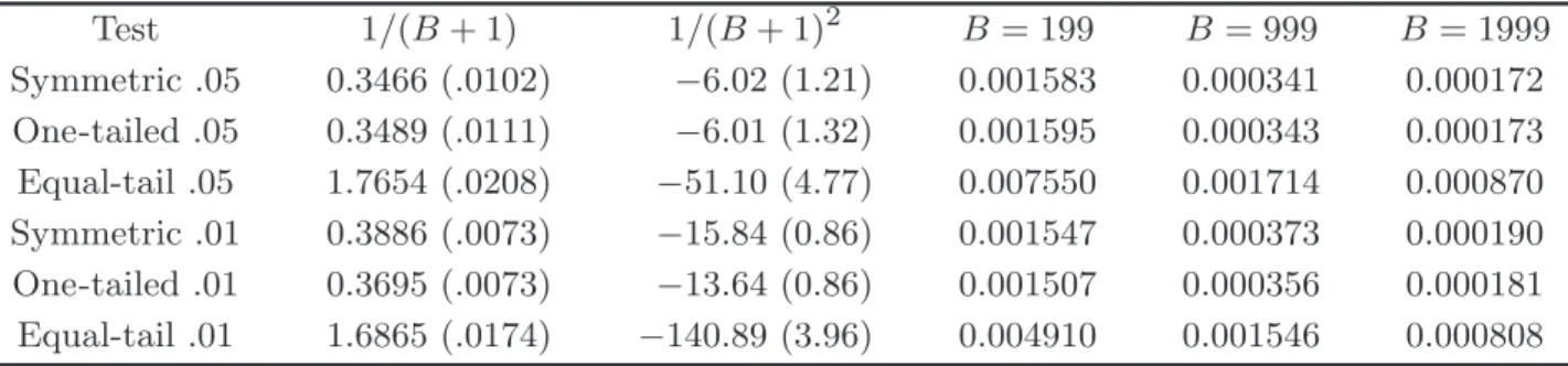
with no constant term. These regressions fit extremely well. Results for tests at the .05 and .01 levels are presented in Table 1. There are 54 experiments for the one-tailed and symmetric tests and 47 experiments for the equal-tail tests. There are fewer experiments for the latter because values of B for which α(B + 1) is an integer but (α/2)(B + 1) is not (namely, 99 and 299) cannot be used. Since each experiment uses 1 million replications, the experimental error should be very small.
Table 1. Response surface regressions for FDB overrejection as a function of B
Test 1/(B+ 1) 1/(B+ 1)2 B= 199 B= 999 B= 1999 Symmetric .05 0.3466 (.0102) −6.02 (1.21) 0.001583 0.000341 0.000172 One-tailed .05 0.3489 (.0111) −6.01 (1.32) 0.001595 0.000343 0.000173 Equal-tail .05 1.7654 (.0208) −51.10 (4.77) 0.007550 0.001714 0.000870 Symmetric .01 0.3886 (.0073) −15.84 (0.86) 0.001547 0.000373 0.000190 One-tailed .01 0.3695 (.0073) −13.64 (0.86) 0.001507 0.000356 0.000181 Equal-tail .01 1.6865 (.0174) −140.89 (3.96) 0.004910 0.001546 0.000808
In addition to coefficients and standard errors, Table 1 shows the fitted values from each of the regressions forB = 199, B = 999, andB = 1999. It can be seen
that all the FDB tests, especially the equal-tail ones, tend to overreject whenB is small. Precisely why this is happening is not clear, although it is probably related to the way in which quantiles are estimated. This is a problem for studies of the finite-sample properties of FDB tests, which must avoid using small values of B. In practice, however, overrejection should not be a problem, because any sensible investigator will use a large value ofB whenever the bootstrap P value is not well above, or well below, the level of the test; see Davidson and MacKinnon (2000b) for a discussion of how to chooseB sequentially when it is expensive to calculate bootstrap test statistics.
6. Relations with the Double Bootstrap
The genuine double bootstrap, as originally laid out in Beran (1988), bootstraps, not the RPcA procedure, but rather the much more expensive conventional
proce-dure described at the beginning of Section 4. Again the idea is to estimate the RP of the single bootstrap test for a nominal level equal to the single bootstrap P value. Briefly, one proceeds as follows. After having computed the realization ˆτ of the statistic τ and the realization ˆµ of the bootstrap DGP from the real data, one uses B1 first-level bootstrap samples to compute bootstrap statistics τj∗ for
j = 1, . . . , B1. If we assume as usual that τ is approximately U(0,1), the next step
is to calculate the first-level bootstrap P value ˆp∗(ˆτ) according to (19).
Each first-level bootstrap sample is also used to generate a second-level bootstrap DGP µ∗∗
j , which is then used to generate B2 bootstrap samples from which we
compute second-level bootstrap test statistics τ∗∗
jl for l = 1, . . . , B2. For the jth
first-level bootstrap sample, the second-level bootstrap P value is ˆ p∗∗j = 1 B2 B2 X l=1 I(τjl∗∗ < τj∗); (25)
compare (11). Thedouble-bootstrap P valueis the proportion of the ˆp∗∗
j that are less than ˆp∗(ˆτ): ˆ p∗∗(ˆτ) = 1 B1 B1 X j=1 I¡pˆ∗∗j ≤pˆ∗(ˆτ)¢. (26)
The inequality in (26) is not strict, because there may well be cases for which ˆ
p∗∗
j = ˆp∗(ˆτ). For this reason, it is desirable that B2 6=B1.
If ˆτ, the τ∗
j, and the τjl∗∗ all come from the same distribution, then it follows
that, for B1 =B2 =∞, the double bootstrap yields exactly the same inferences
as the single bootstrap. Suppose, instead, that the bootstrapping process causes the distribution of the τ∗
j to contain fewer extreme values than the distribution
of τ itself. Therefore, the P values associated with moderately extreme values of ˆ
τ are too small. But it is reasonable to expect that the distributions of the τ∗∗
jl
contain even fewer extreme values than the distribution of theτ∗
j. Therefore, the
ˆ p∗∗
j should tend to be too small, at least for small values of ˆp∗(ˆτ). This implies that
the double-bootstrap P value ˆp∗∗(ˆτ) will be larger than ˆp∗(ˆτ), which is exactly
what we want. By a similar argument, ˆp∗∗(ˆτ) will tend to be smaller than ˆp∗(ˆτ)
when the distribution of theτ∗
j contains more extreme values than the distribution
of τ itself. The same intuition applies as well to the FDB.
Of course, even the double bootstrap cannot be expected to work perfectly. Just as the first-level bootstrap distribution may provide an inadequate approximation to the distribution ofτ underµ0, so may the distribution of the second-level bootstrap
P values provide an inadequate approximation to that of the first-level P values. In principle, any bootstrap procedure, including the double bootstrap, may or may not provide an acceptable approximation to the trueP value associated with ˆτ. The advantage of the double bootstrap, relative to the new FDB procedure, is that it does not require any sort of independence between the bootstrap DGP and the test statistic. But this comes at an enormous computational cost. For each of B1 bootstrap samples, we need to compute B2 + 1 test statistics. Thus the
total number of test statistics that must be computed is 1 +B1 +B1B2. Even
if B2 is somewhat smaller than B1, as is often recommended, this will be vastly
more expensive than computing 1 + 2B test statistics, for reasonable values of B ≈ B1 and B2 ≤ B1. For example, if B = B1 = 999 and B2 = 399, the
FDB procedure involves computing 1999 test statistics, while the genuine double bootstrap involves computing no fewer than 399,601 of them.
7. Tests for Omitted Variables in Probit Models
In this section and the next two, we present results from a number of simulation experiments designed to see whether the procedures proposed in this paper can work well enough to be useful in practice. In this section, we focus on whether
c
RPA and RPfA provide good approximations to the actual rejection probabilities
for single bootstrap tests based on ˆp∗, and on whether the FDB procedure can yield
bootstrap tests with smaller errors in rejection probability than single bootstrap tests.
We begin by studying the OPG version of the LM test for omitted variables in the probit model. This test has noticeably worse finite-sample properties than other tests of the same hypothesis, such as the LR test and the efficient score version of the LM test; see Davidson and MacKinnon (1984). Therefore, it should rarely be used in practice. However, its poor finite-sample performance makes it a good example for the study of alternative bootstrap procedures.
The probit model we study can be written as
E(yt|Xt) = Φ(X1tβ1+X2tβ2), (27)
where yt is a binary dependent variable that can equal 0 or 1, Φ(·) is the
cumu-lative standard normal distribution function, Xt = [X1t X2t] is a 1×k vector of
exogenous variables, with k = k1 +k2, β1 is a k1--vector, and β2 is a k2--vector.
The null hypothesis is that β2 =0. The OPG test statistic is the explained sum
of squares from a regression of ann--vector of 1s on the derivatives of the contri-butions to the loglikelihood with respect to each of the parameters, evaluated at
the ML estimates under the null hypothesis. See Davidson and MacKinnon (1984) for more details.
We report experimental results for two different cases. In Case 1, k1 = 2, k2 = 6,
and β1>= [0 1]. The number of restrictions, k2, is relatively large because the
finite-sample performance of the test becomes worse as k2 increases, and
pre-liminary experiments revealed that the finite-sample performance of the single bootstrap test does likewise. In Case 2, k1 = 2, k2 = 8, and β1>= [1 2]. With
these parameter values, the bootstrap test performs worse because there are more restrictions, the probit model fits better, and the proportion of 0s in the sample is much less than one-half.
For each of the two cases, we perform 161 experiments, with 100,000 replications each, for all sample sizes between 40 and 200. The exogenous variables, other than the constant, are redrawn from the standard normal distribution for each replication, so as to avoid undue dependence on the design matrix. In these experiments, rejection frequencies of the asymptotic test and approximate rejection probabilities of the bootstrap test (bothRPcAandRPfA) are estimated. In addition,
we perform 17 much more expensive experiments, forn= 40,50,60, . . . ,200, also with 100,000 replications, in which we estimate the actual performance of the bootstrap test and the FDB test using B= 999. The results of these experiments are presented graphically in Figures 1 through 3.
Figure 1 shows the rejection frequencies for the asymptotic tests, which always overreject severely, much more so for Case 2 than for Case 1. As expected, the overrejection gradually diminishes as the sample size increases, after an initial increase for Case 2, but it remains quite substantial even at n= 200.
40 50 60 70 80 90 100 110 120 130 140 150 160 170 180 190 200 0.00 0.05 0.10 0.15 0.20 0.25 0.30 0.35 0.40 0.45 0.50 ...... ...... ...... ... ...... ...... ... ...... ...... .. Case 1 Case 2 n
Figure 1. Asymptotic rejection frequencies at .05 level for probit OPG test
40 50 60 70 80 90 100 110 120 130 140 150 160 170 180 190 200 0.038 0.040 0.042 0.044 0.046 0.048 0.050 0.052 0.054 ... ...... ...... ... ... ...... ......... ... ... ......... ... ... ...... ......... ... ... ... ... ...... ... ... ...... ... ......... ...... ... ............ ... ... ... ... ... ... ... ...... ... ...... ...... ... ... ... ......... ...... ... ......... ... ... ... ... ... ...... ... ... ......... ... ... ... ......... ... ......... ... ... ......... ... ... ...... ... ... ... ......... ... ...... ...... ......... ... ... ......... ... ... c RPA ...... ... ... ... .......... .......... ... ... .......... ... ...... .... ... .. ...... ... ...... ... ......... ... .......... ... ... ...... .......... ......... ... ......... ... ......... ... ... f RPA Bootstrap • • • • • • • • • • • • • • • • • • • • FDB ? ? ? ? ? ? ? ? ? ? ? ? ? ? ? ? ? ? ? ? n
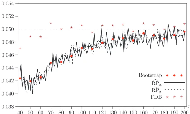
Figure 2. Bootstrap rejection frequencies at .05 level for probit OPG test, Case 1
Figures 2 and 3 pertain to Cases 1 and 2, respectively. Each of these figures shows the rejection frequencies for the (single) bootstrap and FDB tests, along with the approximate rejection probabilities given by RPcA and RPfA. Compared
with the asymptotic tests, the bootstrap tests always perform remarkably well. However, they may either underreject or overreject for small sample sizes and then underreject for a range of somewhat larger sample sizes. The reason for the initial overrejection in Case 2 is explained below. Moreover, as can be seen from the figures, the approximationsRPcAandRPfAare almost always very good indeed,
except for the very smallest sample size.
In Section 4, we discussed the relationship between the variances ofRPcA,RPfA, and
the estimated rejection probability for the asymptotic test. In order to investigate this matter, we regress both estimates of bootstrap rejection probability errors on a number of powers of n−1/2 (with no constant, since asymptotically there is no
error) for each of the two cases. The standard errors of the preferred regressions are estimates of the magnitude of experimental error. For RPcA, these standard
errors are 0.000869 and 0.001004 for Cases 1 and 2, respectively. For RPfA, the
corresponding standard errors are 0.000650 and 0.000765. Thus it appears that, as expected,RPfAcan produce results with noticeably less experimental error than
c
RPA.
In almost all cases, the FDB test outperforms the single bootstrap test. This is most noticeable for the smallest sample sizes and, in Case 2, for the larger sample sizes where the single bootstrap test systematically underrejects. The few cases in which FDB does not perform better seem to occur when both methods perform very well, and some of them can probably be attributed to experimental error.
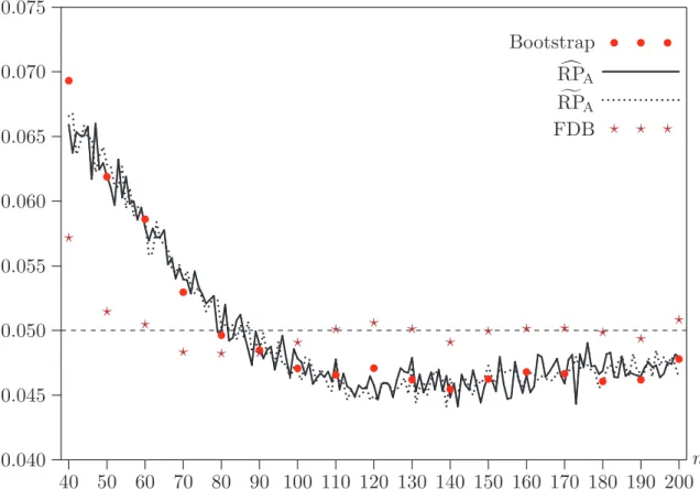
40 50 60 70 80 90 100 110 120 130 140 150 160 170 180 190 200 0.040 0.045 0.050 0.055 0.060 0.065 0.070 0.075 ......... ...... ... ... ... ... ...... ......... ... ...... ... ... ...... ...... ......... ... ............... ............ ... ... ... ... ... ...... ... ......... ...... ... ... ... ... ... ... c RPA ...... ... ......... ......... ...... ....... ... ........... .......... .......... .................... ............... ......... ... f RPA Bootstrap • • • • • • • • • • • • • • • • • • • • FDB ? ? ? ? ? ? ? ? ? ? ? ? ? ? ? ? ? ? ? ? n
Figure 3. Bootstrap rejection frequencies at .05 level for probit OPG test, Case 2
The tendency of the single bootstrap test to overreject in very small samples for Case 2 has a simple explanation. In these cases, ML estimation of the null model not infrequently achieves a perfect fit. When this happens, the test statistic is equal to zero. As is well known, probit models tend to fit too well in small samples. Therefore, the slope coefficients used to generate the bootstrap samples tend to be larger than the ones used to generate the original samples; see MacKinnon and Smith (1998). This means that perfect fits are achieved more often for the bootstrap samples than they are for the original samples. In consequence, there are fewer large values of theτ∗
j than there are of theτj, and the bootstrapP values are
therefore biased downwards. This problem tends to go away rapidly asnincreases.
Table 2. Rejection frequencies at .05 level, 10,000 replications
n B1 B2 Bootstrap FDB Double Bootstrap
Case 1 40 399 199 0.0402 0.0447 0.0462 Case 1 80 399 199 0.0447 0.0502 0.0511 Case 1 160 399 199 0.0514 0.0543 0.0531 Case 2 40 399 199 0.0685 0.0564 0.0330 Case 2 80 399 199 0.0503 0.0496 0.0500 Case 2 160 399 199 0.0488 0.0519 0.0527
We calculate genuine double bootstrap P values in a few experiments. Despite having only 10,000 replications, with B1 = 399 and B2 = 199, these experiments
are far more expensive than any of the others. Table 2, in which these results are reported, provides no evidence to suggest that double bootstrapP values are any more accurate than FDB P values. In Case 2 with 40 observations, where perfect fits occur with some frequency, the double bootstrap actually performs substantially less well. In the other five cases, bearing in mind that the standard errors of the estimated rejection frequencies are roughly 0.0022, there is little to choose between them.
8. Tests for Serial Correlation
The simulation experiments of the second set concern tests for serial correlation. They are designed in part to shed light on the choice between symmetric and equal-tail tests, which can have quite different power properties.
Commonly-used tests for serial correlation are not exact in models with lagged dependent variables or nonnormal disturbances. Consider the linear regression model
yt =Xtβ+γyt−1+ut, ut =ρut−1+εt, εt ∼IID(0, σε2), (28)
where there arenobservations, and Xt is a 1×k vector of observations on
exoge-nous variables. The null hypothesis is that ρ= 0. A simple and widely-used test statistic for serial correlation in this model is thetstatistic on ˆut−1 in a regression
of yt on Xt, yt−1, and ˆut−1. This procedure is proposed in Durbin (1970) and
Godfrey (1978). The test statistic is asymptotically distributed as N(0,1) under the null hypothesis. Since this test can either overreject or underreject in finite samples, it is natural to use the bootstrap in an effort to improve its finite-sample properties.
In order to bootstrap the Durbin-Godfrey test under weak assumptions about the εt, we first estimate the regression in (28) by ordinary least squares. This
yields ˆβ, ˆγ, and a vector of residuals with typical element ˆut. It is then natural to
generate the bootstrap data using the semiparametric bootstrap DGP
yt∗ =Xtβˆ+ ˆγyt∗−1+u∗t, (29)
where the u∗
t are obtained by resampling the vector of rescaled residuals with
typical element (n/(n−k−1))1/2uˆ
t. The initial valuey0∗ is set equal to the actual
pre-sample valuey0. The bootstrap DGP (29) imposes the IID assumption on the
disturbances without imposing any additional distributional assumptions.
In all the reported experiments, the disturbances are normally distributed, the first column of theX matrix is a constant, and the remaining columns are generated by independent, stationary AR(1) processes with normal innovations and parameter ρx. A newX matrix is drawn for each replication. Both asymptotic and bootstrap
rejection frequencies are found to depend strongly onk,ρx,σε, andγ, as well as on
the sample sizen. Since the performance of the asymptotic test improves rapidly as nincreases, n= 20 is used for most of the experiments.
Asymptotic results are based on 200,000 replications for values ofγ between−0.99 and 0.99 at intervals of 0.01. Bootstrap results are based on 100,000 replications for values of γ between −0.9 and 0.9 at intervals of 0.1 using 1999 bootstrap samples. This is an unusually large number to use in a Monte Carlo experiment. It is used because the results in Table 1 suggest that the equal-tail FDB tests will tend to overreject noticeably if B is not quite large.
Results under the null
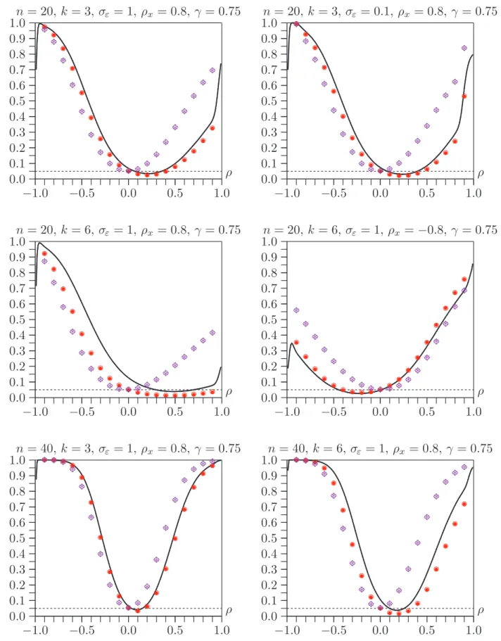
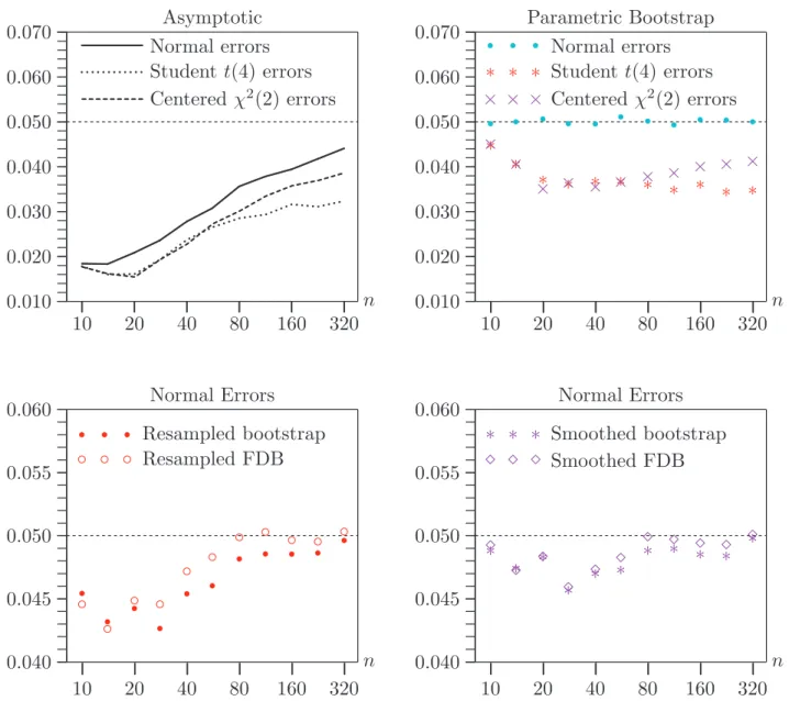
Figure 4 shows three sets of rejection frequencies for the performance of asymptotic and bootstrap tests under the null hypothesis when n = 20. These are represen-tative of the results for a much larger number of similar experiments. Rejection frequencies for tests at the .05 level are shown on the vertical axis, andγ is shown on the horizontal axis. Each row concerns the same set of experiments. Results for the asymptotic test are shown in both panels. The left-hand panel shows re-jection frequencies for symmetric bootstrap and FDB tests, and the right-hand panel shows rejection frequencies for equal-tail bootstrap and FDB tests.
The first row of the figure contains results for a case in which all the bootstrap tests work very well. In the left-hand panel, we see that there is very little difference between the rejection frequencies for the symmetric bootstrap test, based on (2), and for its FDB variant. This is not merely true on average, but also for every replication: The correlation between the two P values is 0.999 for every value ofγ. Thus an investigator who performs both tests would obtain extremely similar results and would probably conclude, correctly, that the bootstrapP value is very reliable.
In the right-hand panel of the first row of the figure, we see that the equal-tail boot-strap test is generally not quite as reliable as the symmetric bootboot-strap test. More-over, the FDB procedure yields noticeably different rejection frequencies which are, in most cases, closer to the nominal level of .05. However, the correlation between the two P values is still very high at approximately 0.996 for all values of γ.
The second and third rows of the figure show results for cases in which, on average, the bootstrap tests do not work as well. In both cases,σ = 10, which is ten times larger than for the case in the first row, andk = 6, which is twice as large. Thus the bootstrap DGP depends on more parameters, and they are estimated less precisely. The only difference between the two cases is thatρx = 0.8 in the second
row, and ρx =−0.8 in the third row.
Several interesting results are evident in the second and third rows of the figure. All four bootstrap tests generally work much better than the asymptotic test on which they are based. It is apparent that a symmetric bootstrap test can overreject when an equal-tail test underrejects, andvice versa. However, the equal-tail tests seem to be a bit more prone to overreject than the symmetric tests. The FDB tests generally work better than the single bootstrap tests, especially when the latter are least reliable. Nevertheless, the correlations between the single bootstrap and FDB tests remain quite high. They are never less than 0.976 for the equal-tail tests and 0.998 for the symmetric ones.
−1.0 −0.5 0.0 0.5 1.0 0.03 0.04 0.05 0.06 0.07 0.08 ... ... ... ... ... ... Asymptotic
. ...
. . .
Symmetric bootstrap ◦ ◦ ◦ ◦ ◦ ◦ ◦ ◦ ◦ ◦ ◦ ◦ ◦ ◦ ◦ ◦ ◦ ◦ ◦ ◦ ◦ ◦ Symmetric FDB γ k = 3,σε = 1, ρx = 0.8 −1.0 −0.5 0.0 0.5 1.0 0.03 0.04 0.05 0.06 0.07 0.08 ... ... ... ... ... ... Asymptotic ∗ ∗ ∗ ∗ ∗ ∗ ∗ ∗ ∗ ∗ ∗ ∗ ∗ ∗ ∗ ∗ ∗ ∗ ∗ ∗ ∗ ∗ Equal-tail bootstrap ¦ ¦ ¦ ¦ ¦ ¦ ¦ ¦ ¦ ¦ ¦ ¦ ¦ ¦ ¦ ¦ ¦ ¦ ¦ ¦ ¦ ¦ Equal-tail FDB γ k = 3, σε = 1, ρx = 0.8 −1.0 −0.5 0.0 0.5 1.0 0.00 0.02 0.04 0.06 0.08 0.10 0.12 ... ... ... ...... ......... ... Asymptotic. . . ...
. . .
Symmetric bootstrap ◦ ◦ ◦ ◦ ◦ ◦ ◦ ◦ ◦ ◦ ◦ ◦ ◦ ◦ ◦ ◦ ◦ ◦ ◦ ◦ ◦ ◦ Symmetric FDB γ k = 6, σε= 10, ρx = 0.8 −1.0 −0.5 0.0 0.5 1.0 0.00 0.02 0.04 0.06 0.08 0.10 0.12 ... ... ... ...... ......... ... Asymptotic ∗ ∗ ∗ ∗ ∗ ∗ ∗∗ ∗ ∗ ∗∗ ∗ ∗ ∗ ∗ ∗ ∗ ∗ ∗ ∗ ∗ Equal-tail bootstrap ¦ ¦ ¦ ¦ ¦ ¦ ¦ ¦ ¦ ¦ ¦ ¦ ¦ ¦ ¦ ¦ ¦ ¦ ¦ ¦ ¦ ¦ Equal-tail FDB γ k = 6, σε = 10,ρx = 0.8 −1.0 −0.5 0.0 0.5 1.0 0.00 0.02 0.04 0.06 0.08 0.10 0.12 ... ... ... ... ... Asymptotic. ...
. . . .
. . .
Symmetric bootstrap ◦ ◦ ◦ ◦ ◦ ◦ ◦ ◦ ◦ ◦ ◦ ◦ ◦ ◦ ◦◦ ◦ ◦ ◦ ◦ ◦ ◦ Symmetric FDB γ k = 6, σε= 10, ρx =−0.8 −1.0 −0.5 0.0 0.5 1.0 0.00 0.02 0.04 0.06 0.08 0.10 0.12 ... ... ... ... ... Asymptotic ∗ ∗ ∗∗ ∗ ∗ ∗ ∗ ∗ ∗ ∗ ∗ ∗ ∗ ∗ ∗ ∗ ∗ ∗ ∗ ∗ ∗ Equal-tail bootstrap ¦ ¦ ¦ ¦ ¦ ¦ ¦ ¦ ¦ ¦ ¦ ¦ ¦ ¦ ¦ ¦ ¦ ¦ ¦ ¦ ¦ ¦ Equal-tail FDB γ k = 6, σε = 10,ρx =−0.8Figure 4. Durbin-Godfrey test rejection frequencies at .05 level under the null,n= 20
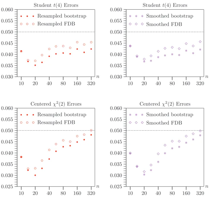
It is of interest to see how fast the performances of the single bootstrap and FDB tests improve as the sample size increases. Figure 5 contains six panels, comparable
0.035 0.040 0.045 0.050 0.055 0.060 0.065 ... ... ...... ...... ...... ...... ...... 10 20 40 80 160 320
. . . .
. . .
Symmetric bootstrap ◦ ◦ ◦ ◦ ◦ ◦ ◦ ◦ ◦ ◦ ◦ ◦ ◦ ◦ Symmetric FDB n k = 3, σε = 1, ρx = 0.8, γ = 0.6 0.035 0.040 0.045 0.050 0.055 0.060 0.065 ... ... ...... ...... ...... ...... ...... 10 20 40 80 160 320 ∗ ∗ ∗ ∗ ∗ ∗ ∗ ∗ ∗ ∗ ∗ ∗ ∗ ∗ Equal-tail bootstrap ¦ ¦ ¦ ¦ ¦ ¦ ¦ ¦ ¦ ¦ ¦ ¦ ¦ ¦ Equal-tail FDB n k = 3, σε = 1, ρx = 0.8, γ = 0.6 0.035 0.040 0.045 0.050 0.055 0.060 0.065 ... ... ...... ...... ...... ...... ...... 10 20 40 80 160 320.
.
. .
.
.
. . . . .
. . .
Symmetric bootstrap ◦ ◦ ◦ ◦ ◦ ◦ ◦ ◦ ◦ ◦ ◦ ◦ ◦ ◦ Symmetric FDB n k = 6, σε= 10, ρx = 0.8, γ = 0.4 0.035 0.040 0.045 0.050 0.055 0.060 0.065 ... ... ...... ...... ...... ...... ...... 10 20 40 80 160 320 ∗ ∗ ∗ ∗ ∗ ∗ ∗ ∗ ∗ ∗ ∗ ∗ ∗ ∗ Equal-tail bootstrap ¦ ¦ ¦ ¦ ¦ ¦ ¦ ¦ ¦ ¦ ¦ ¦ ¦ ¦ Equal-tail FDB n k = 6, σε= 10, ρx = 0.8, γ = 0.4 0.035 0.040 0.045 0.050 0.055 0.060 0.065 ... ... ...... ...... ...... ...... ...... 10 20 40 80 160 320. .
.
. . .
. . . . .
. . .
Symmetric bootstrap ◦ ◦ ◦ ◦ ◦ ◦ ◦ ◦ ◦ ◦ ◦ ◦ ◦ ◦ Symmetric FDB n k = 6, σε = 10, ρx =−0.8, γ = 0.75 0.035 0.040 0.045 0.050 0.055 0.060 0.065 ... ... ...... ...... ...... ...... ...... 10 20 40 80 160 320 ∗ ∗ ∗ ∗ ∗ ∗ ∗ ∗ ∗ ∗ ∗ ∗ ∗ ∗ Equal-tail bootstrap ¦ ¦ ¦ ¦ ¦ ¦ ¦ ¦ ¦ ¦ ¦ ¦ ¦ ¦ Equal-tail FDB n k = 6, σε = 10, ρx =−0.8, γ = 0.75Figure 5. Durbin-Godfrey test rejection frequencies at .05 level under the null
to those in Figure 4. In each of these experiments,γ is fixed at a value associated
with relatively poor performance of at least one of the tests for n = 20, and n takes on the values 10, 14, 20, 28, 40, 56, 80, 113, 160, 226, and 320. Each of these sample sizes is larger than the previous one by a factor of approximately √2. As before, there are 100,000 replications, and B= 1999.
The left-hand panel of the first row shows that the symmetric bootstrap and FDB tests work extremely well for all sample sizes when k = 3 and σε = 1. There is
essentially nothing to choose between them. However, as can be seen from the right-hand panel, the equal-tail tests tend to underreject for very small values of n in this case, with the FDB tests underrejecting less severely than the single bootstrap tests.
The next two rows of the figure, in whichk = 6 andσε = 10, are more interesting.
We see both noticeable overrejection and noticeable underrejection by the single bootstrap tests. With a few exceptions, the FDB tests perform substantially better than the single bootstrap tests when the latter perform badly. The results in the right-hand panel of the second row and the left-hand panel of the third row are particularly dramatic. In these cases, the gain from using the FDB procedure is quite substantial.
It appears that the equal-tail FDB tests overreject slightly for large values of n. This appears to be a manifestation of the phenomenon seen in Table 1. Since the magnitude of the overrejection is just about what we would expect from the results in Table 1, allowing for a certain amount of experimental error, it would surely be even smaller if B were larger than 1999.
Results under the alternative
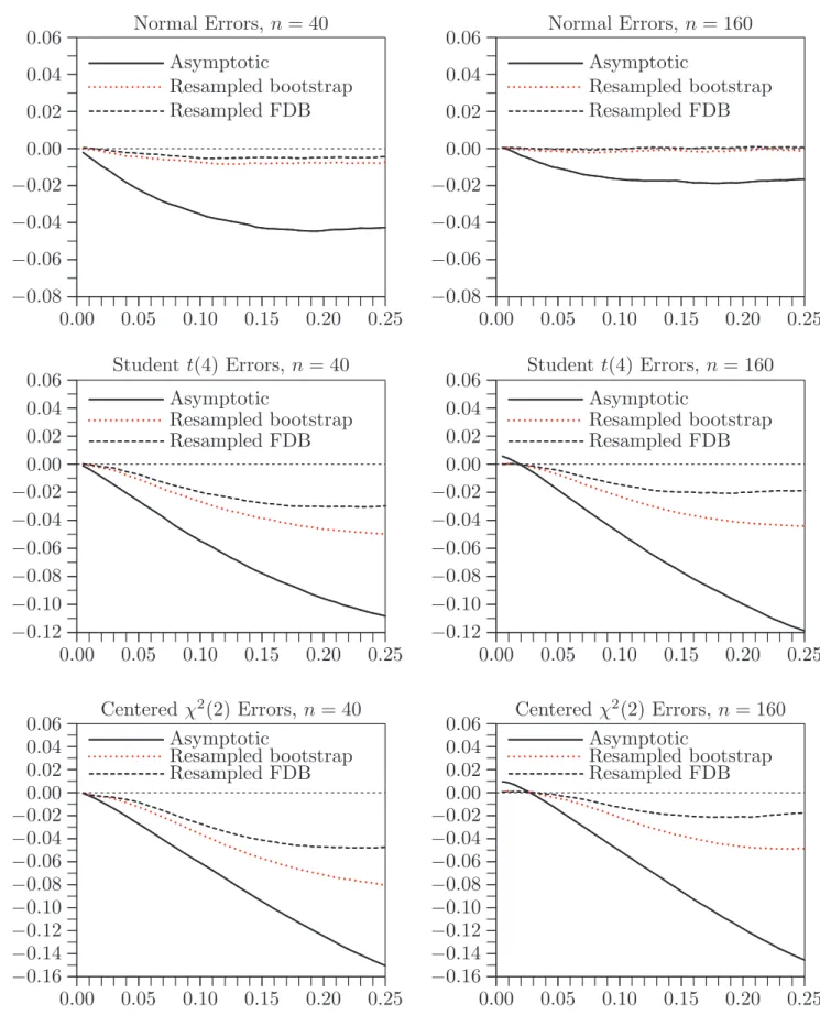
Figure 6 shows power functions for six sets of experiments. The value of ρ is on the horizontal axis, and the rejection frequency is on the vertical axis. Asymptotic results are based on 200,000 replications for 199 values of ρ between −0.99 and 0.99, and bootstrap results are based on 100,000 replications for 19 values of ρ between −0.9 and 0.9. Every panel shows results for both symmetric and equal-tail tests. Because the single bootstrap and FDB tests always have essentially the same power, their symbols always overlap. Thus it may not be immediately apparent that the same symbols are used as in Figures 4 and 5.
In the first two rows of the figure, n = 20. In the four panels in these rows, the shapes of the asymptotic power functions differ dramatically from the inverted bell shape that they must have asymptotically. The power functions for the symmetric bootstrap tests always have essentially the same shape as those for the asymptotic tests, although with a vertical displacement that is quite large in the case of the left-hand panel in the second row. This vertical displacement arises because the asymptotic test overrejects quite severely under the null hypothesis. The symmetric bootstrap test, which does not overreject, inevitably has noticeably less power against all alternatives.
In contrast, the shapes of the power functions for the equal-tail bootstrap tests are dramatically different from the ones for the symmetric bootstrap tests. The former have somewhat less power in whichever direction the asymptotic tests have high power, but they have much more power in the other direction. Specifically,
−1.0 −0.5 0.0 0.5 1.0 0.0 0.1 0.2 0.3 0.4 0.5 0.6 0.7 0.8 0.9 1.0 ... ... ... ... ... ...... ...... ...... ...... ...... ...... ... ... ... ... ... ... ... ...
. .
.
.
.
.
.
. ...
. .
.
◦ ◦ ◦ ◦ ◦ ◦ ◦ ◦ ◦ ◦ ◦ ◦ ◦ ◦ ◦◦◦ ◦◦ ∗ ∗ ∗ ∗ ∗ ∗ ∗ ∗ ∗ ∗ ∗ ∗∗ ∗ ∗ ∗ ∗ ∗∗ ¦ ¦ ¦ ¦ ¦ ¦ ¦ ¦ ¦ ¦ ¦ ¦¦ ¦ ¦ ¦ ¦¦ ¦ ρ n= 20, k = 3, σε= 1, ρx = 0.8, γ = 0.75 −1.0 −0.5 0.0 0.5 1.0 0.0 0.1 0.2 0.3 0.4 0.5 0.6 0.7 0.8 0.9 1.0 ... ... ... ... ...... ...... ...... ...... ...... ...... ... ... ... ... ... ... ... ... .... .
.
.
.
.
.
. .
. ...
.
.
.
◦ ◦ ◦ ◦ ◦ ◦ ◦ ◦ ◦ ◦ ◦ ◦ ◦ ◦ ◦◦◦ ◦ ◦ ∗ ∗ ∗ ∗ ∗ ∗ ∗ ∗ ∗ ∗ ∗ ∗∗ ∗ ∗ ∗ ∗ ∗ ∗ ¦ ¦ ¦ ¦ ¦ ¦ ¦ ¦ ¦ ¦ ¦ ¦¦ ¦ ¦ ¦ ¦¦ ¦ ρ n= 20,k = 3, σε = 0.1, ρx = 0.8, γ = 0.75 −1.0 −0.5 0.0 0.5 1.0 0.0 0.1 0.2 0.3 0.4 0.5 0.6 0.7 0.8 0.9 1.0 ... ... ... ...... ...... ...... ...... ... ...... ... ..........
.
.
.
.
.
. .
. ...
◦ ◦ ◦ ◦ ◦ ◦ ◦ ◦ ◦ ◦ ◦ ◦ ◦ ◦ ◦ ◦ ◦ ◦ ◦ ∗ ∗ ∗ ∗ ∗ ∗ ∗ ∗ ∗ ∗ ∗ ∗ ∗∗∗ ∗∗ ∗∗ ¦ ¦ ¦ ¦ ¦ ¦ ¦ ¦ ¦ ¦ ¦ ¦ ¦¦ ¦¦ ¦¦ ¦ ρ n= 20, k = 6, σε= 1, ρx = 0.8, γ = 0.75 −1.0 −0.5 0.0 0.5 1.0 0.0 0.1 0.2 0.3 0.4 0.5 0.6 0.7 0.8 0.9 1.0 ... ... ...... ......... ... ... ... ... ... ... ... ....
.
. .
. ...
.
.
.
.
.
.
.
◦ ◦ ◦ ◦ ◦ ◦ ◦ ◦ ◦ ◦ ◦◦ ◦◦ ◦ ◦ ◦ ◦◦ ∗ ∗ ∗ ∗ ∗ ∗ ∗ ∗ ∗ ∗ ∗ ∗ ∗∗ ∗ ∗ ∗ ∗ ∗ ¦ ¦ ¦ ¦ ¦ ¦ ¦ ¦ ¦ ¦ ¦ ¦ ¦¦ ¦ ¦ ¦ ¦ ¦ ρ n= 20,k = 6, σε = 1,ρx =−0.8, γ = 0.75 −1.0 −0.5 0.0 0.5 1.0 0.0 0.1 0.2 0.3 0.4 0.5 0.6 0.7 0.8 0.9 1.0 ... ...... ...... ...... ...... ...... ...... ... ... ... ... ... ... ... ... ... ... ... .... . ..
.
.
.
.
.
. ..
.
.
.
.
.
. .
◦ ◦ ◦ ◦ ◦ ◦ ◦ ◦ ◦ ◦ ◦ ◦ ◦ ◦ ◦ ◦ ◦ ◦◦ ∗ ∗ ∗∗ ∗ ∗ ∗ ∗ ∗ ∗ ∗ ∗ ∗ ∗ ∗ ∗∗ ∗ ∗ ¦ ¦ ¦¦ ¦ ¦ ¦ ¦ ¦ ¦ ¦ ¦ ¦ ¦ ¦ ¦¦ ¦ ¦ ρ n= 40, k = 3, σε= 1, ρx = 0.8, γ = 0.75 −1.0 −0.5 0.0 0.5 1.0 0.0 0.1 0.2 0.3 0.4 0.5 0.6 0.7 0.8 0.9 1.0 ... ...... ...... ...... ...... ...... ...... ... ... ... ... ... ... ... ... ... ... ... .... . ..
.
.
.
.
. ...
.
.
.
.
.
◦ ◦ ◦◦ ◦ ◦ ◦ ◦ ◦ ◦ ◦ ◦ ◦◦ ◦ ◦ ◦ ◦ ◦ ∗ ∗ ∗ ∗ ∗ ∗ ∗ ∗ ∗ ∗ ∗∗ ∗ ∗ ∗ ∗ ∗∗ ∗ ¦ ¦ ¦ ¦ ¦ ¦ ¦ ¦ ¦ ¦ ¦ ¦ ¦ ¦ ¦ ¦ ¦¦ ¦ ρ n= 40,k = 6, σε = 1,ρx = 0.8,γ = 0.75Figure 6. Power of Durbin-Godfrey tests at .05 level
when ρx and γ are both positive, the equal-tail tests always have more power
against positive values ofρthan the symmetric tests, and the differences are often dramatic. Since this is a case that we might expect to encounter quite frequently, this is an important result.
In the third row of Figure 6, n = 40. Increasing the value of n brings the shape of the asymptotic power functions much closer to the inverted bell shape that they should have, as can be seen by comparing the left-hand panel in the top row with the left-hand panel in the bottom row and the left-hand panel in the middle row with the right-hand panel in the bottom row. However, it does not change the results about the power of the symmetric and equal-tail bootstrap tests. The equal-tail tests have somewhat less power against negative values ofρ and a great deal more power against positive values