Nonparametric estimation for a stochastic volatility
model.
Fabienne Comte, Valentine Genon-Catalot, Yves Rozenholc
To cite this version:
Fabienne Comte, Valentine Genon-Catalot, Yves Rozenholc. Nonparametric estimation for a
stochastic volatility model.. Finance and Stochastics, Springer Verlag (Germany), 2010, 14 (1),
pp.49-80.
<
10.1007/s00780-009-0094-z
>
.
<
hal-00200874
>
HAL Id: hal-00200874
https://hal.archives-ouvertes.fr/hal-00200874
Submitted on 21 Dec 2007
HAL
is a multi-disciplinary open access
archive for the deposit and dissemination of
sci-entific research documents, whether they are
pub-lished or not.
The documents may come from
teaching and research institutions in France or
abroad, or from public or private research centers.
L’archive ouverte pluridisciplinaire
HAL
, est
destin´
ee au d´
epˆ
ot et `
a la diffusion de documents
scientifiques de niveau recherche, publi´
es ou non,
´
emanant des ´
etablissements d’enseignement et de
recherche fran¸cais ou ´
etrangers, des laboratoires
publics ou priv´
es.
hal-00200874, version 1 - 21 Dec 2007
(will be inserted by the editor)
Nonparametric estimation for a stochastic volatility model.
F. Comte · V. Genon-Catalot · Y. RozenholcReceived: 2007
Corresponding author: F. Comte, MAP5 UMR 8145, Universit´e Paris Descartes,
45 rue des Saints-P`eres,
75270 Paris cedex 06, FRANCE. email: [email protected]
Abstract Consider discrete time observations (Xℓδ)1≤ℓ≤n+1 of the processX
satis-fyingdXt=√VtdBt, withVta one-dimensional positive diffusion process independent of the Brownian motionB. For both the drift and the diffusion coefficient of the un-observed diffusion V, we propose nonparametric least square estimators, and provide bounds for their risk. Estimators are chosen among a collection of functions belonging to a finite dimensional space whose dimension is selected by a data driven procedure. Implementation on simulated data illustrates how the method works. December 21, 2007
Keywords Diffusion coefficient·Drift·Mean square estimator ·Model selection· Nonparametric estimation·Penalized contrast·Stochastic volatility
Mathematics Subject Classification (2000) 62G08·62M05·62P05
1 Introduction
In this paper, we consider a bivariate process (Xt, Vt)t≥0with dynamics described by
the following equations:
dXt=√VtdBt, X0= 0,
dVt=b(Vt)dt+σ(Vt)dWt V0=η, Vt>0, for allt≥0, (1) where (Bt, Wt)t≥0is a standard bidimensional Brownian motion andηis independent
of (Bt, Wt)t≥0. Our aim is to propose and study nonparametric estimators ofb(.) and
σ2(.) on the basis of discrete time observations of the processX only.
F. Comte E-mail: [email protected] ·V. Genon-Catalot E-mail:
[email protected]·Y. Rozenholc E-mail: [email protected]
Model (1) was introduced by Hull and White (1987) under the name of Stochastic Volatility model. It is often adopted in finance to model stock prices, stock indexes or short term interest rates: see for instance Hull and White (1987), Anderson and Lund (1997), the review of Stochastic Volatility models in Ghyselset al.(1996) or the recent book by Shephard (2005) and the references therein. See also an econometric analysis of the subject in Barndorff-Nielsen and Shephard (2002).
The approach to study model (1) is often parametric: the unknown functions are specified up to a few unknown parameters, see the popular examples of Heston (1993) or Cox, Ingersoll and Ross (1985). General statistical parametric approaches of the problem are studied in Genon-Catalot et al.(1999), Hoffmann (2002), Gloter (2007), A¨ıt-Sahalia and Kimmel (2007). A nonparametric estimation of the stationary density ofVtis studied in Comte and Genon-Catalot (2006). A recent proposal for nonparamet-ric estimation of the drift and diffusion coefficients ofV can be found in Ren´o (2006), who studies the empirical performance of a Nadaraya-Watson kernel strategy on two parametric simulated examples. Our approach is new and different, and it is based on a nonparametric mean square strategy. We consider the same probabilistic and sam-pling settings as Gloter (2007) and follow the ideas developed in Comteet al. (2006, 2007), where direct or integrated discrete observations of the process (Vt) are consid-ered. Here, our assumptions ensure that (Vt) is stationary and we consider discrete time observations (Xℓδ)1≤ℓ≤n+1 of the process (Xt) in the so-called high frequency context: δ is small, n is large and nδ =T, the time interval where observations are taken, is large.
We assume thatn=kNand define as it is usual, fori= 0,1, . . . , N−1, the realized quadratic variation associated with (Xℓδ)ik+1≤ℓ<(i+1)k:
ˆ ¯ Vi=kδ1 kX−1 j=0 X(ik+j+1)δ−X(ik+j)δ2.
Setting∆=kδ, ˆV¯i provides an approximation of the integrated volatility: ¯ Vi= 1 ∆ Z (i+1)∆ i∆ Vsds, (2)
which in turn may be, for well chosen k, δ, a satisfactory approximation of Vi∆. We have in mind to obtain regression-type equations, forℓ= 1,2:
Yi(+1ℓ) =f(ℓ)( ˆV¯i) + noise + remainder, where f(1)=b, Yi(1)= ˆ ¯ Vi+1−Vˆ¯i ∆ andf (2)=σ2, Y(2) i = 3 2 ( ˆV¯i+1−Vˆ¯i)2 ∆ . (3)
Choosing a collection of finite dimensional spaces, we use the regression-type equations to construct estimators on these spaces. Then, we propose a data driven procedure to select a relevant estimation space in the collection. As it is usual with these methods, the risk of an estimator ˜f off=borσ2is measured viaE(kf−f˜k2
N) wherekf−f˜k2N = (1/N)PNi=0−1(f−f˜)2( ˆV¯i). We obtain risk bounds which can be interpreted as n, N tend to infinity,δ, ∆tend to 0 andT =nδ=N ∆tends to infinity. These bounds are compared with Hoffmann’s (1999) minimax rates in the case of direct observations of
V. For what concernsb, our method leads to the best rate that can be expected. For what concerns σ2, no benchmark is available in this asymptotic framework. Indeed, Gloter (2000) and Hoffmann (2002) only treat the case of observations within a fixed length time interval, in a parametric setting. As it is always the case, the rates are different for the two functions.
The paper is organized as follows. Section 2 describes the assumptions on the model and the collection of estimation spaces. In Section 3, the estimators are defined and their risks are studied. Section 4 completes the procedure by the data driven selection of the estimation space. Examples of models and simulation results are presented in Section 5. Lastly, proofs are gathered in Section 6.
2 The assumptions
2.1 Model assumptions.
Let (Xt, Vt)t≥0be given by (1) and assume that only discrete time observations ofX,
(Xℓδ)1≤ℓ≤n+1 are available. We want to estimate the drift functionband the square
of the diffusion coefficient σ2 when V is stationary and exponentially β-mixing. We assume that the state space of (Vt) is a known open interval (r0, r1) ofR+and consider
the following set of assumptions. [A1 ] 0≤r0< r1≤+∞,
◦
I= (r0, r1), withσ(v)>0, for allv∈
◦
I. LetI= [r0, r1]∩R.
The functionbbelongs toC1(I),b′is bounded onI,σ2∈C2(I), (σ2)′σis Lipschitz on I, (σ2)′′is bounded onIandσ2(v)≤σ21 for allvinI.
[A2 ] For all v0, v ∈
◦
I, the scale density s(v) = exph−2Rvv 0b(u)/σ
2(u)dui satisfies
R
r0s(x)dx = +∞ =
Rr1
s(x)dx, and the speed density m(v) = 1/(σ2(v)s(v)) satisfiesRr1
r0 m(v)dv=M <+∞.
[A3 ]η∼πand∀i,E(η2i)<∞, whereπ(v)dv= (m(v)/M)1I(r0,r1)(v)dv.
[A4 ] The process (Vt) is exponentiallyβ-mixing,i.e., there exist constantsK >0, θ >0, such that, for allt≥0,βV(t)≤Ke−θt.
Under [A1]-[A3], (Vt) is strictly stationary with marginal distribution π, ergodic andβ-mixing,i.e.limt→+∞βV(t) = 0. Here,βV(t) denotes theβ-mixing coefficient of (Vt) and is given by
βV(t) =
Z r1
r0
π(v)dvkPt(v, dv′)−π(v′)dv′kT V.
The normk.kT V is the total variation norm andPtdenotes the transition probability of (Vt) (see Genon-Catalotet al.(2000)). To prove our main result, we need the stronger mixing condition [A4], which is satisfied in most standard examples. Under [A1]-[A4], for fixed∆, ( ¯Vi)i≥0is a strictly stationary process. And we have:
Proposition 2.1 Under[A1]-[A4], for fixedkandδ,( ˆV¯i)i≥0is strictly stationary and
2.2 Spaces of approximation
The functionsbandσ2 are estimated only on a compact subsetAof the state space
◦
I. For simplicity and without loss of generality, we assume from now on that
A= [0,1], and we set bA=b1A, σA=σ1A. (4) To estimate f = b, σ2, we consider a family Sm, m ∈ Mn of finite dimensional subspaces ofL2([0,1]) and compute a collection of estimators ˆfmwhere for allm, ˆfm belongs toSm. Afterwards, a data driven procedure chooses among the collection of estimators the final estimator ˆfmˆ.
We consider here simple projection spaces, namely trigonometric spaces,Sm, m∈
Mn. The spaceSm is linearly spanned in L2([0,1]) by ϕ1, . . . , ϕ2m+1 withϕ1(x) =
1[0,1](x),ϕj(x) =√2 cos(2πjx)1[0,1](x) for evenj’s andϕj(x) =√2 sin(2πjx)1[0,1](x)
for odd j’s larger than 1. We have Dm = 2m+ 1 = dim(Sm) ≤ Dn and Mn =
{1,3, . . . ,Dn}. The largest space in the collection has maximal dimension Dn, which is subject to constraints appearing later.
Actually, the theory requires smooth bases and regular wavelet bases would also be adequate.
In connection with the collection of spacesSm, we need an additional assumption on the marginal density of the stationary process ( ˆV¯i)i≥0:
[A5 ] The process ( ˆV¯i)i≥0 admits a stationary densityπ∗ and there exist two positive
constantsπ∗0andπ1∗(independent ofn, δ) such that∀m∈ Mn,∀t∈Sm,
π0∗ktk2≤E(t2( ˆV¯0))≤π1∗ktk2. (5)
The existence of the density π∗ is easy to obtain. The checking of (5) is more technical. See the discussion on [A5] in Section 6.2. Below, we use the notations:
ktk2π∗= Z t2(x)π∗(x)dx, ktk2= Z 1 0 t2(x)dx and ktk∞= sup x∈[0,1]| t(x)|. (6)
3 Mean squares estimators of the drift and volatility
3.1 Regression equations
Reminding of (3), we first prove the developments, forℓ= 1,2:
Yi(+1ℓ) =f(ℓ)( ˆV¯i) +Zi(+1ℓ) +R(ℓ)(i+ 1), (7) where the Zi(ℓ)’s are noise terms (with martingale properties) and the R(ℓ)(i)’s are negligible residual terms given in Section 6. For the noise terms, we have, for ℓ= 1 (f(1)=b): Zi(1)= 1 ∆2 Z (i+2)∆ i∆ ψi∆(u)σ(Vu)dWu+ (ui+1,k−ui,k)/∆, with
and ui,k=∆1 kX−1 j=0 Z (ik+j+1)δ (ik+j)δ √ VsdBs !2 − Z (ik+j+1)δ (ik+j)δ Vsds .
Note that ˆV¯i= ¯Vi+ui,k.
On the other hand, forℓ= 2 (f(2)=σ2), we haveZi(2)=Zi(2,1)+Z(2i ,2)+Zi(2,3)with
Zi(2,1)= 3 2∆3 Z (i+2)∆ i∆ ψi∆(s)σ(Vs)dWs !2 − Z (i+2)∆ i∆ ψi∆2 (s)σ2(Vs)ds , Zi(2,2)= 3 ∆b(Vi∆) Z (i+2)∆ i∆ ψi∆(s)σ(Vs)dWs + 3 ∆3 Z (i+2)∆ i∆ Z (i+2)∆ s ψ2i∆(u)du ! [(σ2)′σ](Vs)dWs,
whereψi∆ is given in (8), and Zi(2,3)= 3
∆( ¯Vi+1−V¯i)(ui+1,k−ui,k).
3.2 Mean squares contrast
Equation (7) gives a natural regression equation to estimatef(ℓ). In light of this, we consider the following contrast, for a function t ∈ Sm where Sm is a space of the collection and forℓ= 1,2:
γ(Nℓ)(t) = 1
N NX−1
i=0
[Yi(+1ℓ)−t( ˆV¯i)]2. (9) Then the estimators are defined as
ˆ
fm(ℓ)= arg min t∈Smγ
(ℓ)
N (t). (10)
The minimization ofγN(ℓ)overSmusually leads to several solutions. In contrast, the ran-domRN-vector ( ˆfm(ℓ)( ˆV¯0), . . . ,fˆm(ℓ)( ˆV¯N−1))′ is always uniquely defined. Indeed, let us
denote byΠmthe orthogonal projection (with respect to the inner product ofRN) onto the subspace ofRN,{(t( ˆV¯0), . . . , t( ˆV¯N−1))′, t∈Sm}, then ( ˆfm(ℓ)( ˆV¯0), . . . , fm(ℓ)( ˆV¯N−1))′=
ΠmY(ℓ)whereY(ℓ)= ( ¯Y1(ℓ), . . . , YN(ℓ))′. This is the reason why we consider a properly defined risk for ˆfm(ℓ)based on the design points, i.e.
E " 1 N NX−1 i=0 ( ˆfm(ℓ)( ˆV¯i)−f( ˆV¯i))2 # .
Thus, the error is measured via the riskE(kfˆm(ℓ)−f(ℓ)k2N) where
ktk2N = 1 N NX−1 i=0 t2( ˆV¯i).
Let us mention that for a deterministic functionE(ktk2N) =ktk2π∗ =
R
t2(x)π∗(x)dx. Moreover, under Assumption [A5], the normsk.kandk.kπ∗are equivalent for functions
inSm(see notations (6)).
The following decomposition of the contrast holds:
γN(ℓ)(t)−γN(ℓ)(f(ℓ)) =kt−f(ℓ)k2N − 2 N NX−1 i=0 (Yi(+1ℓ) −f(ℓ)( ˆV¯i))(f(ℓ)−t)( ˆV¯i) In view of (7), we define the centered empirical processes, forℓ= 1,2:
νN(ℓ)(t) = 1
N NX−1
i=0
t( ˆV¯i(ℓ))Zi(+1ℓ),
and the residual process:
R(Nℓ)(t) = 1
N NX−1
i=0
t( ˆV¯i)R(ℓ)(i+ 1). Then we obtain that
γN(ℓ)(t)−γN(ℓ)(f(ℓ)) =kt−f(ℓ)k2N −2νN(ℓ)(t−f
(ℓ))
−2R(Nℓ)(t−f(ℓ)).
Letfm(ℓ)be the orthogonal projection off(ℓ)onSm. Write simply thatγN(ℓ)( ˆfm(ℓ))≤ γN(ℓ)(fm(ℓ)) by definition of the estimator, and therefore thatγN(ℓ)( ˆf
(ℓ) m )−γ(Nℓ)(f(ℓ)) ≤ γN(ℓ)(fm(ℓ))−γN(ℓ)(f(ℓ)). This yields kfˆm(ℓ)−f(ℓ)k2N ≤ kfm(ℓ)−f(ℓ)kN2 + 2νN(ℓ)( ˆf (ℓ) m −fm(ℓ)) + 2R(Nℓ)( ˆfm(ℓ)−fm(ℓ)). The functions ˆfm(ℓ)andfm(ℓ)beingA-supported, we can cancel the termskf1IAck2
N that appears in both sides of the inequality. Therefore, we get
kfˆm(ℓ)−fA(ℓ)k2N ≤ kfm(ℓ)−fA(ℓ)kN2 + 2νN(ℓ)( ˆf
(ℓ)
m −fm(ℓ)) + 2R(Nℓ)( ˆfm(ℓ)−fm(ℓ)). (11) Taking expectations and finding upper bounds for
E( sup
t∈Sm,ktk=1
[νN(ℓ)(t)]2) and E( sup t∈Sm,ktk=1
[R(Nℓ)(t)2) will give the rates for the risks of the estimators.
3.3 Risk for the collection of drift estimators
For the estimation ofb, we obtain the following result.
Proposition 3.1 Assume thatN ∆≥1and1/k≤∆. Assume that[A1]-[A5]hold and consider a modelSmin the collection of models withDn≤O(√N ∆/ln(N))whereDn
is the maximal dimension (see Section 2.2). Then the estimatorfˆm(1)= ˆbmoff(1)=b
is such that
E(kˆbm−bAk2n)≤7kbm−bAk2π∗+KE
(σ2(V0))Dm N ∆ +K
′∆, (12) wherebA=b1I[0,1] andK, K′ andK”are some positive constants.
Note that the condition onDnimplies that√N ∆/ln(N) must be large enough. It follows from (12) that it is natural to select the dimensionDmthat leads to the best compromise between the squared bias termkbm−bAk2π∗ (which decreases when
Dmincreases) and the variance term of orderDm/(N ∆).
Now, let us consider the classical high frequency data setting: let∆=∆n,k=kn andN=Nn be, in addition, such that∆n→0,N=Nn→+∞, Nn∆n/ln2(Nn)→ +∞when n → +∞and that 1/(kn∆n) ≤ 1. Assume for instance that bA belongs to a ball of some Besov space,bA ∈ Bα,2,∞([0,1]),α≥1, and that kbm−bAk2π∗ ≤
π∗1kbm−bAk2, thenkbA−bmk2π∗ ≤C(α, L, π1∗)D−m2α, forkbAkα,2,∞≤L(see Lemma
12 in Barronet al.(1999)). Therefore, if we chooseDm= (Nn∆n)1/(2α+1), we obtain
E(kˆbm−bAk2n)≤C(α, L)(Nn∆n)−2α/(2α+1)+K′∆n. (13) The first term (Nn∆n)−2α/(2α+1) =Tn−2α/(2α+1)is the optimal nonparametric rate proved by Hoffmann (1999) for direct observation ofV.
Now, let us find conditions under which the last term is negligible. For instance, under the standard condition ∆n = O(1/(Nn∆n)), the term ∆n is negligible with respect to (Nn∆n)−2α/(2α+1).
Now, consider the choiceskn= 1/∆nandδn=n−c. Let us see if there are possible choices of c for which all our constraints are fulfilled. To havenδn → +∞ requires 0< c <1. As∆n=knδn =δn/∆n, we have∆n =√δn=n−c/2and Nn=n/kn = n1−c/2. Thus,∆n →0 andNn, Nn∆n→+∞. Finally, the last constraint to fulfill is that Nn∆2n = n1−3c/2 =O(1). Thus for 2/3 ≤c < 1, the dominating term in (13) is (Nn∆n)−2α/(2α+1), i.e. the minimax optimal rate. We have obtained a possible “bandwidth” of stepsδn.
3.4 Risk for the collection of volatility estimators
For the collection of volatility estimators, we have the result
Proposition 3.2 Assume that [A1]-[A5] hold and consider a model Sm in the
col-lection of models with maximal dimensionDn ≤O(√N ∆/ln(N)). Assume also that 1/k≤∆andN ∆≥1,∆≤1. Then the estimatorfˆm(2)= ˆσ2moff(2)=σ2is such that
E(kσˆm2 −σA2k2N)≤7kσ2m−σA2k2π∗+KE
(σ4(V0))Dm
N +K
′
Res(Dm, k, ∆), (14)
where the residual term is given by
Res(Dm, k, ∆) =Dm2∆2+Dm5∆3+D 3 m k2 + 1 k2∆2, (15)
whereσA2 =σ21I[0,1], andK,K′ are some positive constants.
The discussion on rates is much more tedious. Consider the asymptotic setting de-scribed forb. Assume thatσA2 belongs to a ball of some Besov space,σA2 ∈ Bα,2,∞([0,1]),
and thatkσm2 −σ2Ak2π∗ ≤π∗1kσ2m−σA2k2, thenkσ2A−σ2mk2π∗ ≤C(α, L, π∗1)D−m2α, for
kσ2Akα,2,∞≤L. Therefore, if we chooseDm=Nn1/(2α+1), andkn≤1/∆n, we obtain
The first termNn−2α/(2α+1)is the optimal nonparametric rate proved by Hoffmann (1999) whenNn discrete time observations ofV are available.
For the second term, let us set kn =na,∆n =n−b,δn = n−c, and recall that nδn=Nn∆nandn/Nn=kn, so thatNn=n1−a anda+b=c. We look fora, bsuch that
Res(Nn1/(2α+1), kn, ∆n)≤Nn−2α/(2α+1).
For this, we take 1/(k2n∆2n) =Nn−2α/(2α+1)which implies 2(a−b)/(1−a) = 2α/(2α+1). We get
a=(2α+ 1)c+α 5α+ 2 , b=
(3α+ 1)c−α
5α+ 2 . Then we imposeNn2/(2α+1)∆n2 ≤Nn−2α/(2α+1)which is equivalent to
2b≥[(2α+ 2)/(2α+ 1)](1−a)⇒c≥(3α+ 2)[2(2α+ 1)].
NextNn5/(2α+1)∆n3 ≤Nn−2α/(2α+1) leads to
3b≥[(2α+ 5)/(2α+ 1)](1−a)⇒c≥(7α+ 5)/(11α+ 8).
LastlyNn3/(2α+1)/kn2≤Nn−2α/(2α+1)holds for−2a≤ −[(3 + 2α)/(2α+ 1)](1−a),i.e. c≥2(α+ 3)/(6α+ 5).
The optimal dimension has also to fulfillNn1/(2α+1)≤ Dn≤√Nn∆ni.e.−[(2α− 1)/[2(2α+ 1)]](1−a)≤ −b/2 which impliesc≤(5α−2)/(5α). Finally, we must have
c∈ 3α+ 2 2(2α+ 1), 5α−2 5α →α→+∞ 3 4,1 .
This interval is nonempty as soon asα >2.
In terms of the initial numbernof observations, the rate is now (n1−a)−2α/(2α+1) where 1−a is at most 1/2, when α→+∞. This is consistent with Gloter’s (2000) result: in the parametric case, he obtainsn−1/2instead ofn−1 for the quadratic risk.
4 Data driven estimator of the coefficients
The second step is to ensure an automatic selection of Dm, which does not use any knowledge onf(ℓ), and in particular which does not require to know the regularityα. This selection is standardly done by setting
ˆ m(ℓ)= arg min m∈Mn h γn(ℓ)( ˆfm(ℓ)) + pen(ℓ)(m) i , (17)
with pen(ℓ)(m) a penalty to be properly chosen. We denote by ˜f(ℓ)= ˆfm(ˆℓ)(ℓ)the resulting estimator and we need to determine pen such that, ideally,
E(kf˜(ℓ)−fA(ℓ)k2n)≤C inf m∈Mn k fA(ℓ)−fm(ℓ)k2+E(σ 2ℓ(V 0))Dm N ∆2−ℓ ! + negligible terms,
4.1 Result for the data driven estimator ofb
We almost reach this aim for the estimation ofb.
Theorem 4.1 Assume that [A1]-[A5] hold,1/k≤∆, ∆≤1 andN ∆≥1. Consider the collection of models with maximal dimension Dn ≤ O(√N ∆/ln(N)). Then the
estimator˜b= ˆfm(1)ˆ(1) ofbwheremˆ
(1) is defined by (17) with
pen(1)(m)≥κσ12Dm
N ∆, (18)
whereκis a universal constant, is such that
E(k˜b−bAk2n)≤C inf m∈Mn kbm−bAk2π∗+ pen(1)(m) +K ∆+ 1 N ∆+ 1 ln2(N)k∆ . (19) For comments on the practical calibration of the penalty, see Section 5.2.
It follows from (19) that the adaptive estimator automatically realizes the bias-variance compromise, provided that the last terms can be neglected as discussed above. Here, the bandwidth for the choices of δn is slightly narrowed because of a stronger constraint. More precisely, we choose 1/(kn∆n) =∆n (instead of 1 previously), that is kn=∆−n2, so that∆n=knδn=∆−n2δ−n1. Therefore∆n=δn1/3and ifδn=n−c, then ∆n=n−c/3. Also,Nn =n/kn =n1−2c/3,Nn∆n =nδn =n1−c,Nn∆2n=n1−4c/3. Hence if 3/4< c <1, we have altogether:Nn,Nn∆n/ln2(Nn) tend to infinity withn, ∆n,Nn∆2ntend to zero.
In that case, whenever bA belongs to some Besov ball (see (13)), and if kbm− bAk2π∗ ≤π1∗kbm−bAk2, then ˜bachieves the optimal corresponding nonparametric rate. Note that, in the parametric framework, Gloter (2007) obtains an efficient estimation ofbin the same asymptotic context.
4.2 Result for the data driven estimator of the volatility We can prove the following Theorem.
Theorem 4.2 Assume that [A1]-[A5] hold, 1/k ≤ ∆, ∆ ≤ 1 and N ∆ ≥ 1. Con-sider the collection of models with maximal dimension Dn ≤√N ∆/ln(N). Then the
estimator ˜σ2= ˆfm(2)ˆ(2) ofσ
2wheremˆ(2)is defined by (17) with
pen(2)(m)≥κσ14Dm
N , (20)
whereκis a universal constant, is such that
E(kσ˜2−σA2k2N)≤C inf m∈Mn kσ2m−σ2Ak2π∗+ pen(2)(m) +C′Resg(N, k, ∆), (21) where g Res(N, k, ∆) =N ∆3+N5/2∆11/2+(N ∆) 3/2 k2 + 1 k2∆2. (22)
Now, ifσ2Abelongs to a ball of some Besov space, σ2A∈ Bα,2,∞([0,1]), then auto-matically, inf m∈Mn kσm2 −σA2k2π∗+ pen(2)(m) =O(Nn−2α/(2α+1)) without requiring the knowledge ofα. Therefore,
E(k˘σm2˘ −σ2Ak2N)≤C(α, L)Nn−2α/(2α+1)+C′Resg(Nn, kn, ∆n).
It remains to study the residual term. Notice that we do not know the optimal min-imax rate for estimating σ2, under our set of assumptions on the models and on the asymptotic framework. However, Gloter (2000) and Hoffmann (2002), with observa-tions within a fixed length time interval, obtain the parametric rate n−1/2 (in vari-ance). Taking this as a benchmark, we try to make the residual less than O(n−1/2). Let us set kn =na, ∆n =n−b, henceNn =n/kn =n1−a and Nn∆n =n1−(a+b). This yields that 1−a−3b,(5−5a−11b)/2,(3−7a−3b)/2,2(b−a) must all be less than or equal to−1/2, in association witha+b <1 andNn1/(2α+1)≤√Nn∆n. This set of constraint is not empty (e.g.a= 9/16, b= 5/16 fits).
5 Examples and numerical simulation results
In this section, we consider examples of diffusions and implement the estimation algo-rithm on simulated data for the stochastic volatility modelX given by (1).
5.1 Simulated paths
We consider the processesVt(i) for i= 1, . . . ,4 specified by the couples of functions
bi, σi2,i= 1, . . . ,4: 1. b1(x) =x
−θln(x) +12c2, σ12(x) =c2x2which corresponds to exp(Ut) forUtan Ornstein-Uhlenbeck process, dUt=−θUtdt+cdWt. Whatever the chosen step,Ut is exactly simulated as an autoregressive process of order 1. We took θ = 1 and
c= 0.75.
2. b2(x) =b0(x−2),σ22(x) =σ20(x−2), whereb0(x) =−(1−x2)
h
c2x+θ2ln1+1−xxi andσ02(x) =c(1−x2) are the diffusion coefficients of the process th(Ut) (th(x) = (ex−e−x)/(ex+e−x), with the same parameters as for case 1). The processVt(2)
corresponds to th(Ut) + 2 which is a positive bounded process.
3. b3(x) =x(b0(ln(x)) +12σ02(ln(x))) andσ23(x) =x2σ02(ln(x)) which corresponds to
the processVt(3)= exp(th(Ut)).
4. b4(x) = dc2/4−θx, σ42(x) = c2x which corresponds to the Cox-Ingersoll-Ross
process. A discrete time sample is obtained in an exact way by taking the Euclidean norm of ad-dimensional Ornstein-Uhlenbeck process with parameters −θ/2 and
c/2. We tookd= 9,θ= 0.75 andc= 1/3.
We obtain samples of discrete observations of the processes (Vℓδ(j′))1≤ℓ≤N′ for j =
1, . . . ,4 withδ′=δ/10,N′δ′=T, from which we generate (Xℓδ(j))1≤ℓ≤n, by using that
Xℓδ−X(ℓ−1)δ =
sZ ℓδ
(ℓ−1)δ
k= 150 k= 200 k= 250 k= 300 k= 500
b mean 1,70.10−3 1,87.10−3 1,95.10−3 2,1.10−3 2,91.10−3
(std) (5,38.10−4) (5,06.10−4) (4,93.10−4) (4,92.10−4) (4,68.10−4)
σ2 mean 14,8.10−5 6,23.10−5 8,77.10−5 15,3.10−5 28,6.10−5
(std) (3,26.10−5) (2,26.10−5) (3,74.10−5) (4,0.10−5) (3,39.10−5)
Table 1 Mean squared errors (with standard deviations in parenthesis) for the estimation of
bandσ2, 100 paths of the CIR process, different values ofkfor the quadratic variation, when
using the trigonometric basis.
Process Vt(1)[T] V (2) t [T] V (3) t [T] V (4) t [T] V (4) t [GP] b mean 4,08.10−2 7,51.10−2 7,05.10−2 1,95.10−3 1,04.10−3 (std) (6,89.10−3) (8,56.10−3) (8,12.10−3) (4,93.10−4) (2,89.10−4) σ2 mean 1,42.10−1 1,89.10−2 8,32.10−2 8,77.10−5 4,61.10−5 (std) (3,47.10−2) (1,54.10−3) (1,61.10−2) (3,74.10−5) (3,19.10−5)
Table 2 Mean squared errors (with standard deviations in parenthesis) for the estimation of
b and σ2, 100 paths of the processesVt(i),i = 1, . . . ,4 when using the trigonometric basis
(except the last column, piecewise polynomial basis),k= 250.
with (εℓ) i.i.d.N(0,1) independent of (Vs, s≥ 0). Approximations of the integrated processes are computed by discrete integration (with a trapeze method).
The generatedVjδ(i′),i= 1, . . . ,4 samples have lengthN
′ = 5.106, for a stepδ′ =
1000/5.106= 2.10−4, and the integrated process is computed using 10 data, therefore, we obtainn= 5.105andδ= 2.10−3, forT =nδ= 1000. Different values ofkare used, but the best value,k= 250, corresponds to∆=kδ= 0.5 andN = 2000 data for the sameT.
5.2 Estimation algorithms and numerical results
We use the algorithm of Comte and Rozenholc (2004). The precise calibration of penal-ties is difficult and done for the trigonometric basis but also for a general piecewise polynomial basis, described in detail in Comteet al(2006). Additive correcting terms are involved in the penalty. Such terms avoid under-penalization and are in accordance with the fact that the theorems provide lower bounds for the penalty. The correcting terms are asymptotically negligible and do not affect the rate of convergence. For the trigonometric polynomial collection (denoted by [T]), the drift penalty (i= 1) and the diffusion penalty (i= 2) are given by
2sˆ 2 i n Dm+ ln2.5(Dm+ 1) , withDmat most [N ∆/ln1.5(N)].
For the penalty when considering general piecewise polynomial bases (denoted by [GP]), we refer the reader to Comte et al. (2006). The constantsκ1 and κ2 in both
drift and diffusion penalties have been set equal to 2. The term ˆs21replacesσ12/∆for
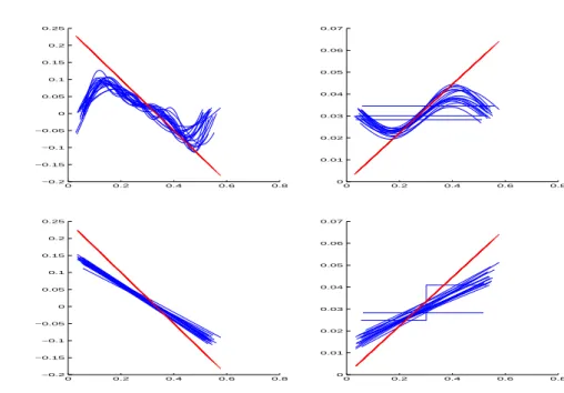
0 0.2 0.4 0.6 0.8 −0.2 −0.15 −0.1 −0.05 0 0.05 0.1 0.15 0.2 0.25 0 0.2 0.4 0.6 0.8 0 0.01 0.02 0.03 0.04 0.05 0.06 0.07 0 0.2 0.4 0.6 0.8 −0.2 −0.15 −0.1 −0.05 0 0.05 0.1 0.15 0.2 0.25 0 0.2 0.4 0.6 0.8 0 0.01 0.02 0.03 0.04 0.05 0.06 0.07
Fig. 1 Estimation ofb(left) andσ2 (right) for 20 paths of the CIR process with the
trigono-metric basis (top) and the piecewise polynomial basis (bottom),k= 250.
how ˆs22is obtained. We run once the estimation algorithm ofσ2with the basis [T] and with a preliminary penalty where ˆs22 is taken equal to 2 maxm(γ(2)n (ˆσ2m)). This gives a preliminary estimator ˜σ20. Afterwards, we take ˆs2 equal to twice the 99.5%-quantile
of ˜σ20. The use of the quantile is here to avoid extreme values. We get ˜σ2. We use this estimate and set ˆs21= max0≤k≤N−1(˜σ2( ˆV¯k))/∆for the penalty ofb. The results given
0 1 2 3 −1 −0.5 0 0.5 0 1 2 3 0 0.5 1 1.5 2 2.5
Fig. 2 Estimation ofb (left) andσ2 (right) for 20 paths of the processVt(1) (exponential
Ornstein Uhlenbeck) with the trigonometric basis,k= 250.
by our algorithm are described in Figure 1 and 2. We plot in Figure 1 the true function (thick curve) and 20 estimated functions (thin curves) in the casebandσ2when using
first the basis [T] and then the basis [GP], in the case of the CIR process. We can see that the trigonometric basis finds the right slope in the central part of the interval, whereas the basis [GP] in general selects only one bin and a straight curve, but with a slightly too small slope. The same type of result holds in Figure 2 for the exponen-tial Orsntein Uhlenbeck process. For comparison with direct or integrated observations of V, we refer to Comteet al. (2006,2007). It is not surprising that in the case of a stochastic volatility model, empirical results are less satisfactory and require a large number of observations.
We also give in Tables 1 and 2 results of Monte-Carlo type experiments. In Table 1, we show the results of the estimation procedure with the basis [T] and the CIR process when choosing different values ofkfor building the quadratic variation. Clearly, there is an optimal value. If k is too large, there are not enough observations left for the estimation algorithm. Ifkis too small, bias phenomena appear, related to the violation of the theoretical assumptions (mainly 1/k≤∆). We repeated the experiment for the other processes and obtained analogous results. In general, for this sample size, the choicek= 250 seems to be relevant. In Table 2, we can see from the last two columns that the basis [GP] seems to be better than [T], at least for the CIR process. The errors are computed as the mean over 100 simulated paths of the empirical errors (e.g. (1/NPNi=0−1[b( ˆV¯i)−˜b( ˆV¯i)]2 forb).
6 Discussion on the assumptions and proofs
6.1 Proof of Proposition 2.1
We start with some preliminaries. LetIt=R0tVsds. The joint process (Vt, It)t≥0is a
two dimensional diffusion satisfying:
dVt=b(Vt)dt+σ(Vt)dWt, V0=η,
dIt=Vtdt, I0= 0
Under regularity assumptions on b and σ, this process admits a transition density, sayqt(v0, i0,;v, i) for the conditional density of (Vt, It) given V0 =v0,I0=i0. This
density is w.r.t. the Lebesgue measure on (0,+∞)2(see Rogers and Williams (2000)). We assume that these assumptions hold.
Now, let us set
Jℓδ =
Z ℓδ
(ℓ−1)δ
Vsds, ℓ≥1. (23) The discrete time process (Vℓδ, Jℓδ)ℓ≥1is strictly stationary and Markov. Its one step
transition operator is given by the density:
(v, j)→qδ(v0,0;v, j) :=qδ(v0;v, j).
Its stationary density is given byR π(v0)dv0qδ(v0;v, j) :=πδ(v, j). Let us set, forℓ≥1,
Zℓ=Xℓδ−X(ℓ−1)δ (24) and defineεℓby the relation:Zℓ=Jℓδ1/2εℓ. Conditionally on (Vt)t≥0, the random
the r.v (εℓ, ℓ ≥1) are i.i.d. with distributionN(0,1) and the sequence (εℓ, ℓ≥1) is independent of (Vt)t≥0. Hence (Zℓ)ℓ≥1and ( ˆV¯i)i≥0are strictly stationary processes.
From the preliminaries and the above remarks, we deduce that the process (Vℓδ, Jℓδ, εℓ)ℓ≥1
is stationary Markov. Itsℓ-step transition operator is given by:
Qℓδ(v0;dv, dj, du) =qδ(ℓ)(v0;v, j)n(u)dvdjdu
whereqδ(ℓ)(v0;v, j) is theℓ-step transition density of (Vℓδ, Jℓδ) andn(u) is the standard gaussian density. The stationary density of (Vℓδ, Jℓδ, εℓ)ℓ≥1isπδ(v, j)n(u). Hence
kQ(δℓ)(v0;dv, dj, du)−πδ(v, j)n(u)dvdjdukT V = Z |qδ(ℓ)(v0, vj)−πδ(v, j))|n(u)dvdjdu = Z |qδ(ℓ)(v0;v, j)−πδ(v, j))|dvdj. We may now use the representation of theβ-mixing coefficient of strictly stationary Markov processes (see e.g. Genon-Catalotet al.(2000)) to compute
βV.δ,J.δ,ε(ℓ) =
Z
πδ(v0, j0)n(u0)du0dv0dj0kQδ(ℓ)(v0;dv, dj, du)−πδ(v, j)n(u)dvdjdukT V =βV.δ,J.δ(ℓ).
Now, we haveβZ(ℓ)≤βV.δ,J.δ,ε(ℓ) =βV.δ,J.δ(ℓ)≤βV((ℓ−1)δ). Finally, βVˆ¯(i)≤βZ(ik)≤βV((ik−1)δ)≤cβV(i∆). 2
6.2 Discussion on the assumptions
Actually, Assumption [A3] is too strong. We only need the existence of moments up to a certain order. Let us now discuss [A5]. Using the representation
ˆ ¯ V0= 1 kδ k X ℓ=1 Jℓδε2ℓ,
we see that ˆV¯0has a conditional density given (Vt, t≥0). Integrating this density w.r.t. the distribution of (Jℓδ, ℓ= 1, . . . , k), we get that ˆV¯0 has a densityπ∗. However the
formula forπ∗ is untractable.
On the other hand, we can obtain (5) by another approach. We have
t2( ¯V0) =t2(V0) + ( ¯V0−V0)(t2)′(V0) + 1 2( ¯V0−V0) 2Z 1 0 (t2)”(V0+u( ¯V0−V0))du.
Now we use that, for anyt∈Sm, there exists some constantCsuch that
k(t2)′k∞≤CDm2ktk2 andk(t2)”k∞≤CD3mktk2.
Noting that|E V¯0−V0|F0|=O(∆), we get|E[( ¯V0−V0)(t2)′(V0)]| ≤CDm2∆ktk2= O(D2m∆). On the other hand,
E " ( ¯V0−V0)2 Z 1 0 (t2)”(V0+u( ¯V0−V0))du # ≤ k(t 2)” k∞E[( ¯V0−V0)2] ≤CD3m∆ktk2.
It follows that|E(t2( ¯V0)−t2(V0))| ≤C∆Dm3ktk2. Next, t2( ˆV¯0) =t2( ¯V0) + ( ˆV¯0−V¯0)(t2)′(V0) + ( ˆV¯0−V¯0)[(t2)′( ¯V0)−(t2)′(V0)] +1 2( ˆV¯0−V¯0) 2Z 1 0 (t2)”( ¯V0+u( ˆV¯0−V¯0))du.
By Gloter’s (2007) Proposition 3.1, we have|E[( ˆV¯0−V¯0)|V0]| ≤cδ(1 +V0)candE[|Vˆ¯0−
¯ V0|2]≤c/k. Hence |E(t2( ˆV¯0)−t2( ¯V0))| ≤Cktk2(∆D2m+ √ ∆D3m √ k + D3m k ). Since 1/k≤∆ |E(t2( ˆV¯0)−t2(V0))| ≤Cktk2∆D3m.
As there exist two positive constants π0, π1 such that∀v∈ A, π0 ≤π(v) ≤π1, we
obtain
(π0−C∆Dn3)ktk2≤ ktkπ2∗ ≤(π1+C∆Dn3)ktk2.
Under the constraint that∆D3n=o(1), we get (5) fornlarge enough. This constraint is compatible with the other ones, see the discussion after Theorem 4.1.
6.3 Definition of the residuals and their properties We have
R(1)(i+ 1) =b( ¯Vi)−b( ˆV¯i) +R∗(1)((i+ 1)∆)
where R(1)∗ is the residual term for bstudied in Comte et al.(2006, Proposition 3.1)
and defined by R∗(1)((i+ 1)∆) =b(V(i+1)∆)−b( ¯Vi) + 1 ∆2 Z (i+3)∆ (i+1)∆ ψ(i+1)∆(s)(b(Vs)−b(V(i+1)∆))ds. On the other hand,
R(2)(i+ 1) = 3 2 (ui+1,k−ui,k)2 ∆ + [σ 2(V (i+1)∆−σ2( ˆV¯i)] +R(2)∗ ((i+ 1)∆)
whereR(2)∗ is the residual term forσ2studied in Comteet al.(2006, Propositions 4.1,
4.2 and 4.3) defined byR(2)∗ =P3m=1R (2,m) ∗ with R∗(2,1)(i∆) = 3 2∆3 Z (i+2)∆ i∆ ψi∆(s)b(Vs)ds !2 R∗(2,2)(i∆) = 3 ∆3 Z (i+2)∆ i∆ ψi∆(u)(b(Vu)−b(Vi∆))du ! Z (i+2)∆ i∆ ψi∆(u)σ(Vu)dWu ! R∗(2,3)(i∆) = 3 2∆3 Z (i+2)∆ i∆ Z (i+2)∆ s ψi∆2 (u)du ! τb,σ(Vs)ds,
where τb,σ= (σ2/2)(σ2)” +b(σ2)′. This decomposition is obtained by applying Ito’s formula and Fubini’s theorem.
We may now summarize the following useful results, proved in Comte et al. (2006, Propositions 3.1, 4.1, 4.2 and 4.3):
Lemma 6.1 Under Assumptions [A1]-[A2]-[A3],
1. Forℓ= 1,2, form= 1,2, for alli,E{[R(∗ℓ)(i∆)]2m} ≤c∆2mℓwherecis a constant. 2. LetZ∗(1)(i) = (1/∆2)
R(i+2)∆
i∆ ψi∆(s)σ(Vs)dWs. For alli,E([Z∗(1)(i)]2)≤(2/3∆)E(σ2(V0)).
3. For alli,E([Zi(2,1)]2)≤c1E(σ4(V0))andE([Z(2i ,2)]2)≤c2σ12∆.
We also need the following result:
Lemma 6.2 Under assumptions [A1]-[A3], for any integeri,E[( ¯Vi−V¯ˆi)2] =E(u2i,k)≤ 2E(V02)/k andE[( ¯Vi−Vˆ¯i)4] =E(u4i,k)≤56E(V04)/k2.
Proof of Lemma 6.2.This follows from Proposition 3.1 p.504 in Gloter (2007).2
6.4 Proof of Propositions 3.1 and 3.2
For sake of brevity, we give both proofs at the same time. The main difference lies in the orders of the expectations and in the appearance of a specific term in the study of the estimator ofσ2. Let us thus defineR(∗∗ℓ)forℓ= 1,2 asR(1)∗∗ =R(1) and
R(2)∗∗(i+ 1) =R(2)(i+ 1)−[σ2(V(i+1)∆−σ2( ˆV¯i)]. Moreover letTN(1)(t) = 0 and
TN(2)(t) = 1
N NX−1
i=0
(σ2(V(i+1)∆−σ2( ˆV¯i))t( ˆV¯i). Let us consider the set
ΩN = ( ω/ ktk2N ktk2 π∗ −1 ≤ 1 2, ∀t∈ ∪m,m′∈Mn(Sm+Sm′)/{0} ) . (25) OnΩN,ktkπ∗ ≤√2ktkN. From (11), we deduce kfˆm(ℓ)−fA(ℓ)k2N ≤ kfm(ℓ)−fA(ℓ)k2N + 1 8kfˆ (ℓ) m −fm(ℓ)k2π∗+ 16 sup t∈Sm,ktkπ∗=1 [νN(ℓ)]2(t) +16 sup t∈Sm,ktkπ∗=1 [TN(ℓ)(t)]2 +1 8kfˆ (ℓ) m −fm(ℓ)k2N+ 8 N NX−1 i=0 [R∗∗(ℓ)(i+ 1)]2 ≤ kfm(ℓ)−fA(ℓ)k2N + 3 8kfˆ (ℓ) m −fm(ℓ)k2N + 16 sup t∈Sm,ktkπ∗=1 [νN(ℓ)]2(t) +16 π∗0t∈Sm,supktk=1 [TN(ℓ)(t)]2+ 8 N NX−1 i=0 [R(∗∗ℓ)(i+ 1)]2.
In the last line above, we use the lower boundπ0∗introduced in [A5]. Setting Bm(0,1) = {t ∈ Sm,ktk = 1} and Bπ
∗
m(0,1) = {t ∈ Sm,ktkπ∗ = 1}, the
following holds on the setΩN: 1 4kfˆ (ℓ) m −fA(ℓ)k 2 N ≤ 7 4kf (ℓ) m −fA(ℓ)k 2 N+16 sup t∈Bπ∗ m(0,1) [νN(ℓ)]2(t)+16 π∗ 0 sup t∈Bm(0,1) [TN(ℓ)(t)]2+8 N NX−1 i=0 [R(∗∗ℓ)(i+1)]2.
Lemma 6.3 Under assumptions [A1]-[A3] and [A5], if1/k≤∆, we have, forℓ= 1,2 E sup t∈Bπ∗ m(0,1) [νN(ℓ)]2(t) ! ≤K CℓDm N ∆2−ℓ, withCℓ=E(σ2ℓ(V0)).
The Lipschitz condition on band Lemma 6.2 imply that
E[(b( ¯Vi)−b( ˆV¯i))2]≤cbE[( ¯Vi−Vˆ¯i)2]≤2cbE(V02)/k.
Consequently, there exists a constantcsuch that
E N8 NX−1 i=0 [R(1)∗∗(i+ 1)]2 ! ≤c(∆+k−1). Thus E(kˆbm−bAk2N1IΩN)≤7kbm−bk2π∗+ 32 π0∗E t∈Sm,supktk=1 [ν(1)N (t)]2 ! +c”(∆+k−1).
By gathering all bounds, we find
E(kˆbm−bk2N1IΩN)≤7kbm−bk2π∗+KE (σ2(V0))Dm N ∆ (1 + 1 k∆) +K ′(∆+k−1).
On the other hand, Lemma 6.1 and Lemma 6.2 imply that
E(1 N NX−1 i=0 [R(2)∗∗(i+ 1)]2≤2E " 1 N NX−1 i=0 [R(2)∗ (i+ 1)]2+ 9 4 (ui+1,k−ui,k)4 ∆2 !# ≤2c∆2+ 36 ∆2E(u 4 1,k)≤C(∆2+ 1 k2∆2).
Next we need to boundE
supt∈Sm,ktk=1[TN(2)(t)]
2. This is obtained in the
fol-lowing Lemma:
Lemma 6.4 Under the Assumptions of Proposition 3.2 and if1/k≤∆, there exists a constantC such that
E sup
t∈Sm,ktk=1
[TN(2)(t)]2
!
≤C(D2m∆2+D5m∆3+D3m/k2+Dm/(N k)). We can use Lemma 6.1 in Comteet al.(2005) to obtain that, ifDn≤C√N ∆/ln(N), then
P(ΩNc )≤ c
N4.
This enables to check thatE(kfˆm(ℓ)−f(ℓ)k2N1IΩc
n) ≤c/N using the same lines as the analogous proof given p.532 in Comteet al.(2007). For this reason, details are omitted.
6.5 Proof of Lemma 6.3.
Caseℓ= 1. Next, let us defineFt=σ((Ws, Bs),0≤s≤t, η).We can use martingale properties to see that,∀t∈Sm,
E(t( ˆV¯i)Zi(1)+1) =E(E(t( ˆV¯i)Zi(1)+1|F(i+1)∆)) =E(t( ˆV¯i)E(Zi(1)+1|F(i+1)∆)) = 0 because the last conditional expectation is zero. Moreover, the same tool shows that the covariance term E(t( ˆV¯i)t( ˆV¯ℓ)Zi(1)+1Z
(1)
ℓ+1) for ℓ ≥ i+ 2 is also null by inserting a
conditional expectation givenF(ℓ+1)∆. Consequently, it is now easy to see that
E sup t∈Sm,ktk=1 [νN(1)(t)]2 ! ≤ Dm X j=1 E[νN2(ϕj)]≤ Dm X j=1 Var " 1 N NX−1 i=0 ϕj( ˆV¯i)Zi(1)+1 # ≤ N2 Dm X j=1 Varϕj( ˆV¯1)Z(1)2 ≤ N2 Dm X j=1 E(ϕ2j( ˆV¯1)Z2(1))2)≤ 2DmE[(Z2(1))2] N .
Now, Lemma 6.2 implies that E[(ui+2,k−ui+1,k)2/∆2 = E[(u2i+2,k+u2i+1,k)/∆2 ≤ c/(k∆2). Then, applying also Lemma 6.1 (ii), it follows that, with
E sup t∈Sm,ktk=1 [νN(1)(t)]2 ! ≤KDm N ∆ 1 + 1 k∆ .
Caseℓ= 2. Next, for the martingale terms, we write
E( sup t∈Bπ∗ m(0,1) [νN(2)(t)]2)≤ 1 π0∗E(t∈Bsupm(0,1) [νN(2)(t)]2)≤ 1 π0∗ Dm X j=1 E([νn(2)(ϕj)]2) = 1 π∗ 0 Dm X j=1 E N1 NX−1 i=0 ϕj( ˆV¯i)Zi(2)+1 !2 ≤ π2∗ 0 Dm X j=1 E 1 N NX−1 i=0 ϕj( ˆV¯i)(Zi(2+1,1)+Z (2,2) i+1 ) !2 + 9 N ∆ NX−1 i=0 ϕj( ˆV¯i)( ¯Vi+2−V¯i)(ui+2,k−ui+1,k) !2
Both terms are bounded separately. For the first one, we use that, forr= 1,2 cov(ϕj( ˆV¯i)Zi(2+1,r), ϕj( ˆV¯ℓ)Zℓ(2+1,r)) = 0
ifℓ≥i+ 2, by inserting a conditional expectation with respect toF(ℓ+1)∆. Now, for r= 1,2, Dm X j=1 E 1 N NX−1 i=0 ϕj( ˆV¯i)Zi(2+1,r) !2 ≤ 1 N2 Dm X j=1 E X 0≤i,ℓ≤N−1 ϕj( ˆV¯i)Zi(2+1,r)ϕj( ˆV¯ℓ)Zℓ(2+1,r) = 1 N2 X j=1 DmE (N−1 X i=0 h ϕ2j( ˆV¯i)[Zi(2+1,r)] 2 +ϕj( ˆV¯i)Zi(2+1,r)ϕj( ˆV¯i+1)Zi(2+2,r) i) ≤ N2k Dm X j=1 ϕj2k∞E[(Z2(2,r))2]≤2Dm N [˜c1E(σ 4(V 0)) + ˜c2∆] by using Lemma 6.1.
For the second part, let us define the filtration generated byBand the whole path ofV, i.e.
GVt =σ(Vs, s∈R+, Bs, s≤t) =σ(Ws, s∈R+, Bs, s≤t, η). Now we observe that
E(t( ˆV¯i)( ¯Vi+2−V¯i+1)ui+1,k) =E h E(t( ˆV¯i)( ¯Vi+2−V¯i+1)ui+1,k)|G(Vi+1)∆) i =E h t( ˆV¯i)( ¯Vi+2−V¯i+1)E(ui+1,k)|G(Vi+1)∆) i = 0
asE(ui+1,k)|G(Vi+1)∆) = 0. Moreover for anyℓ > i,
E(t( ˆV¯i)( ¯Vi+2−V¯i+1)ui+1,kt( ˆV¯ℓ)( ¯Vℓ+2−V¯ℓ+1)uℓ+1,k)) = 0
by inserting a conditional expectation with respect toG(Vℓ+1)∆. The last remark is that one can easilty see that
E[( ¯Vi+1−V¯i)4]≤ 1 ∆4E Z (i+2)∆ (i+1)∆ (Vs−Vs−∆)ds !4 ≤C∆2. Now we have Dm X j=1 E N ∆1 NX−1 i=0 ϕj( ˆV¯i)( ¯Vi+2−V¯i)ui+1,k !2 = 1 N2∆2 Dm X j=1 NX−1 i=0 E ϕ2j( ˆV¯i)( ¯Vi+2−V¯i)2u2i+1,k ≤ N ∆Dm2E 1/2[( ¯V 2−V¯1)4]E1/2[u42,k] ≤CDm N 1 k∆.
The second part of this term can be treated in the same way, and it follows that if 1/k≤∆, then this term is less thanC′Dm/N.2
6.6 Proof of Lemma 6.4.
Let us recall that we know from Comteet al.(2006) that
TN∗(t) = 1 N NX−1 i=0 (σ2(V(i+1)∆−σ2( ¯Vi))t( ¯Vi) is such that E( sup t∈Bm(0,1) [TN∗(t)]2)≤C(D2m∆2+D5m∆3).
Here, we write thatTN(2)(t) =TN(2,1)(t) +TN(2,2)(t) +TN(2,3)(t) +TN∗(t) with
TN(2,1)(t) = 1 N NX−1 i=0 [t( ˆV¯i)−t( ¯Vi)][σ2( ˆV¯i)−σ2( ¯Vi)], TN(2,2)(t) = 1 N NX−1 i=0 t( ¯Vi)[σ2( ˆV¯i)−σ2( ¯Vi)], TN(2,3)(t) = 1 N NX−1 i=0 [t( ˆV¯i)−t( ¯Vi)][σ2( ¯Vi)−σ2(V(i+1)∆)]. We shall use the following decompositions obtained by the Taylor formula:
σ2( ˆV¯i)−σ2( ¯Vi) = ( ˆV¯i−V¯i)(σ2)′( ¯Vi) +Ri, t( ˆV¯i)−t( ¯Vi) = ( ˆV¯i−V¯i)t′( ¯Vi) +Si(t) withE(R2i)≤C/k2andE(R4i)≤C/k4if (σ2)” is bounded, andE
supt∈Bm(0,1)Si(t)2 ≤ CDm5/k2,E1/2 supt∈Bm(0,1)Si(t)4 ≤CD5m/k2 because kt”k2∞ ≤CD5mktk2. Now, the three terms can be studied as follows. First
TN(2,1)(t) = 1 N NX−1 i=0 ( ˆV¯i−V¯i)2(t′)( ¯Vi)(σ2)′( ¯Vi) + 1 N NX−1 i=0 ( ˆV¯i−V¯i)t′( ¯Vi)Ri +1 N NX−1 i=0 ( ˆV¯i−V¯i)(σ2)′( ¯Vi)Si(t) + 1 N NX−1 i=0 RiSi(t) :=TN(2,1,1)(t) +TN(2,1,2)(t) +TN(2,1,3)(t) +TN(2,1,4)(t),
and we bound each term successively. Clearly by Schwarz inequality applied to each term, we find, E( sup t∈Bm(0,1) [TN(2,1,1)(t)]2)≤CE1/2( ¯V14) D3m k2 using thatkt′k2∞≤CDm3ktk2, E( sup t∈Bm(0,1) [TN(2,1,2)(t)]2)≤CD 3 m k3 , E( sup t∈Bm(0,1) [TN(2,1,3)(t)]2)≤CE1/2( ¯V14) D5m k3 , and E( sup t∈Bm(0,1) [TN(2,1,4)(t)]2)≤CD 5 m k4 . Therefore, if 1/k≤∆,E(supt∈Bm(0,1)[TN(2,1)(t)]2)≤C(Dm3/k2+Dm5/k3).
Next, we write that TN(2,2)(t) = 1 N NX−1 i=0 t( ¯Vi)(σ2)′( ¯Vi)( ˆV¯i)−V¯i) +N1 NX−1 i=0 t( ¯Vi)Ri =TN(2,2,1)(t) +TN(2,2,2)(t).
We obtain easily that
E( sup t∈Bm(0,1) [TN(2,2,2)(t)]2)≤E( sup t∈Bm(0,1)k tk2∞N1 N X i=1 R2i)≤Φ20DmE(R21)≤CDm/k2,
a term which is negligible with respect to the previous ones.
Then ( ˆV¯i−V¯i)ψ( ¯Vi) is a martingale increment with respect to the filtration (GtV), for any measurable functionψ. In particular,
E[( ˆV¯i−V¯i)ψ( ¯Vi)] =E[E[( ˆV¯i−V¯i)ψ( ¯Vi)|Gi∆V ]] =E[ψ( ¯Vi)E[( ˆV¯i−V¯i)|Gi∆V ]] = 0 sinceE( ˆV¯i|Gi∆V ) = ¯Vi. In the same way, fori < ℓ,
E
( ˆV¯i−V¯i)ψ( ¯Vi)( ˆV¯ℓ−V¯ℓ)ψ( ¯Vℓ)
= 0
by inserting a conditional expectation with respect toGVℓ∆. Therefore
E( sup t∈Bm(0,1) [TN(2,2,1)(t)]2)≤ Dm X j=1 E N1 NX−1 i=0 ϕj( ¯Vi)(σ2)′( ¯Vi)( ˆV¯i−V¯i) !2 = Dm X j=1 1 NE ϕj( ¯V1)(σ2)′( ¯V1)( ˆV¯1−V¯1 2 ≤ N1E ( Dm X j=1 ϕ2j( ¯V1))[(σ2)′( ¯V1)]2( ˆV¯1−V¯1)2 ≤ DNmE1/2[(σ2)′( ¯V1)4]E1/2[u41,k]≤CE1/2( ¯V14)Dm N k.
For the last term, we writeTN(2,3)(t) =TN(2,3,1)(t) +TN(2,3,2)(t) where
TN(2,3,1)(t) = (1/N) NX−1 i=0 ( ˆV¯i−V¯i)t′( ¯Vi)(σ2( ¯Vi)−σ2(V(i+1)∆)), TN(2,3,2)(t) = (1/N) NX−1 i=0 Si(t)(σ2( ¯Vi)−σ2(V(i+1)∆)).
Moreover, we know from Comte et al. (2006) that E[(σ2( ¯Vi)−σ2(V(i+1)∆))2] ≤
E1/2[(σ2( ¯Vi)−σ2(V(i+1)∆))4]≤C∆. Now, forTN(2,3,1)(t), we proceed as forT
(2,2,1)
N (t)
since both have the same martingale property w.r.t.GVs. We get
E( sup t∈Bm(0,1) [TN(2,3,1)(t)]2)≤ Dm X j=1 E N1 NX−1 i=0 ϕ′j( ¯Vi)( ˆV¯i−V¯i)(σ2( ¯Vi)−σ2(V(i+1)∆)) !2 ≤ N1 Dm X j=1 E (ϕ′j)2( ¯V1)( ˆV¯1−V¯1)2(σ2( ¯V1)−σ2(V2∆))2 ≤ CD 3 m N E 1/2(u4 1,k)E1/2[(σ2( ¯V1)−σ2(V2∆))4] ≤CD 3 m∆ N k
asPj(ϕ′j)2(x)≤CDm3. UsingDm2 ≤N ∆and 1/k≤∆impliesE(supt∈Bm(0,1)[TN(2,3,1)(t)]
2) ≤
CDm∆3. On the other hand,E(supt∈Bm(0,1)[T (2,3,2)
N (t)]
2)
≤CD5m∆/k2≤CD5m∆3, as 1/k≤∆.
By gathering and comparing all terms and assuming that 1/k≤∆, we obtain the bound given in Lemma 6.4.2
6.7 Proof of Theorem 4.1
The proof of this theorem relies on the following Bernstein-type Inequality:
Lemma 6.5 Under the assumptions of Theorem 4.1, for any positive numbers ǫand
v, we have P "N−1 X i=0 t( ˆV¯i)Z((1)i+1)∆≥N ǫ,ktk2N ≤v2 # ≤exp −N ∆ǫ 2 2σ2 1v2 .
Proof of Lemma 6.5: Noting that W is a Brownian motion with respect to the augmented filtrationFs=σ((Bu, Wu), u≤s, η), the proof is obtained as the analogous proof in Comteet al.(2007), Lemma 2 p.533.2
Now we turn to the proof of Theorem 4.1.
As in the proof of Proposition 3.1, we have to splitk˜b−bAk2N =kb˜−bAk2N1IΩN+k˜b− bAk2N1IΩc
N. For the study onΩ c
N, the end of the proof of Proposition 3.1 can be used. Now, we focus on what happens on ΩN. From the definition of ˜b, we have,∀m∈
Mn,γN(ˆbmˆ) + pen( ˆm)≤γN(bm) + pen(m). We proceed as in the proof of Proposition 3.1 with some additional penalty terms and obtain
E(kˆbmˆ −bAk2N1IΩN)≤7kbm−bAk2π∗+ pen(m) + 32E sup
t∈Sm+Sm,ˆ ktkπ∗=1
[νN(1)(t)]21IΩN
!
−E(pen( ˆm)) + 32c′∆.
The difficulty here is to control the supremum of νN(1)(t) on a random ball (which depends on the random ˆm). This is done by settingνN(1)=νN(1,1)+νN(1,2), with
νN(1,1)(t) = 1 N NX−1 i=0 Z((1)i+1)∆t( ˆV¯i), ν(1N,2)(t) = 1 N NX−1 i=0 t( ˆV¯i) u i+2,k−ui+1,k ∆ .
We use the martingale property ofνN(1,1)(t) and a rough bound forνN(1,2)(t) as follows. ForνN(1,2), we simply write, as previously
E sup t∈Sm+Sm,ˆ ktkπ∗=1 [νn(1,2)(t)]2 ! ≤ π1∗ 0 E sup t∈Sn,ktk=1 [νn(1,2)(t)]2 ! ≤ π1∗ 0 Dn X j=1 E[(νN(2)(ϕj))2] ≤ π4D∗n 0N E[(u1,k/∆)2]≤ 4Dn π∗ 0N kn∆2 ≤ 4 π∗ 0 1 kn∆.
ForνN(1,1), let us denote by
Gm(m′) = sup t∈Sm+Sm′,ktkπ∗=1
νN(1,1)(t)
the quantity to be studied. Introducing a functionp(m, m′), we first write
G2m( ˆm)1IΩN ≤[(G2m( ˆm)−p(m,mˆ))1IΩN]++p(m,mˆ)
≤ X
m′∈Mn
[(G2m(m′)−p(m, m′))1IΩN]++p(m,mˆ).
Then pen is chosen such that 32p(m, m′)≤pen(m)+pen(m′). More precisely, the next Proposition determines the choice ofp(m, m′) which in turn will fix the penalty.
Proposition 6.1 Under the assumptions of Theorem 4.1, there exists a numerical constantκ1 such that, forp(m, m′) =κ1σ12(Dm+Dm′)/(n∆), we have
E[(G2m(m′)−p(m, m′))1IΩN]+≤cσ12
e−Dm′
N ∆ .
Proof of Proposition 6.1.The result of Proposition 6.1 follows from the inequality of Lemma 6.5 by theL2-chaining technique used in Baraud et al. (2001b) (see Section 7 p.44-47, Lemma 7.1, withs2=σ12/∆). 2
It is easy to see that the result of Theorem 4.1 follows from Proposition 6.1 with pen(m) =κσ12Dm/(N ∆).2
6.8 Proof of Theorem 4.2
The lines of the proof are the same as the ones of Theorem 4.1. Moreover, they follow closely the analogous proof of Theorem 2 p.524 in Comteet al.(2007), see also Comte
References
1. A¨ıt-Sahalia, Y. and Kimmel,R.: Maximum likelihood estimation of stochastic volatility models. J. Finance Econ.83, 413-452 (2007).
2. Andersen, T., Lund, J.: Estimating continuous-time stochastic volatility models of the short-term interest rate. J. Econom.77, 343-377 (1997).
3. Barndorff-Nielsen, O. E., Shephard, N.: Econometric analysis of realized volatility and its use in estimating stochastic volatility models. J. R. Stat. Soc. Ser. B Stat. Methodol.64, 253–280 (2002).
4. Barron, A.R., Birg´e, L., Massart, P.: Risk bounds for model selection via penaliza-tion.Probab. Theory Related Fields113, 301–413 (1999).
5. Comte, F., Genon-Catalot, V. Penalized projection estimator for volatility density. Scand. J. Statist.33, 875-893 (2006).
6. Comte, F., Genon-Catalot, V., Rozenholc, Y.: Penalized nonparametric mean square estimation of the coefficients of diffusion processes. Bernoulli 13, 514-543 (2007).
7. Comte, F., Genon-Catalot, V., Rozenholc, Y.: Nonparametric estimation for a dis-cretely observed integrated diffusion model. Preprint MAP5, 2006-11 (2006). 8. Comte, F., Rozenholc, Y.: A new algorithm for fixed design regression and
denois-ing. Ann. Inst. Statist. Math.56, 449-473 (2004).
9. Cox, J. C., Ingersoll, J. E., Jr., Ross, S. A.: A theory of the term structure of interest rates. Econometrica53, 385-407 (1985).
10. Genon-Catalot, V., Jeantheau, T., Lar´edo, C.: Parameter estimation for discretely observed stochastic volatility models . Bernoulli5, 855-872 (1999).
11. Genon-Catalot, V., Jeantheau, T., Lar´edo, C.: Stochastic volatility models as hid-den Markov models and statistical applications. Bernoulli,6, 1051-1079 (2000). 12. Ghysels, E., Harvey, A., Renault, E.: Stochastic volatility. In: Maddala, G. (Ed.)
Handbook of Statistics, vol. 14, North-Holland, Amsterdam, 119-191 (1996). 13. Gloter, A.: Estimation of the volatility diffusion coefficient for a stochastic volatility
model. (French) C. R. Acad. Sci. Paris, Sr. I Math.330, 3, 243-248 (2000). 14. Gloter, A.: Efficient estimation of drift parameters in stochastic volatility models.
Finance Stoch.,11, 495-519 (2007).
15. Heston, S.: A closed-form solution for options with stochastic volatility with ap-plications to bond and currency options. Rev. Financial Stud.6, 327-343 (1993). 16. Hoffmann, M.: Adaptive estimation in diffusion processes. Stochastic Process.
Appl.79, 135-163 (1999).
17. Hoffmann, M.: Rate of convergence for parametric estimation in a stochastic volatil-ity model. Stochastic Process. Appl.97, 147-170 2002.
18. Hull, J., White, A.: The pricing of options on assets with stochastic volatility. J. of Finance42, 281-300 (1987).
19. Ren`o, R.: Nonparametric estimation of stochastic volatility models. Economic Let-ters90, 390-395 (2006).
20. Rogers, L.C.G., Williams, D.: Diffusions, Markov processes, and martingales. Vol. 2, Reprint of the second (1994) edition, Cambridge Univ. Press, Cambridge (2000). 21. Shephard, N.: Stochastic volatility. Selected readings. (Advanced texts in