using Cartesian Genetic Programming
Andrew James Turner
PhD
University of York Electronics
Abstract
NeuroEvolution is the application of Evolutionary Algorithms to the training of Artifi-cial Neural Networks. NeuroEvolution is thought to possess many benefits over traditional training methods including: the ability to train recurrent network structures, the capabil-ity to adapt network topology, being able to create heterogeneous networks of arbitrary transfer functions, and allowing application to reinforcement as well as supervised learning tasks.
This thesis presents a series of rigorous empirical investigations into many of these perceived advantages of NeuroEvolution. In this work it is demonstrated that the abil-ity to simultaneously adapt network topology along with connection weights represents a significant advantage of many NeuroEvolutionary methods. It is also demonstrated that the ability to create heterogeneous networks comprising a range of transfer functions represents a further significant advantage.
This thesis also investigates many potential benefits and drawbacks of NeuroEvolution which have been largely overlooked in the literature. This includes the presence and role of genetic redundancy in NeuroEvolution’s search and whether program bloat is a limitation. The investigations presented focus on the use of a recently developed NeuroEvolution method based on Cartesian Genetic Programming. This thesis extends Cartesian Genetic Programming such that it can represent recurrent program structures allowing for the creation of recurrent Artificial Neural Networks. Using this newly developed extension, Recurrent Cartesian Genetic Programming, and its application to Artificial Neural Net-works, are demonstrated to be extremely competitive in the domain of series forecasting.
Contents
Abstract iii
Contents v
List of figures ix
List of tables xiii
Acknowledgements xvii
Declaration xix
1 Introduction 1
1.1 Structure of this Chapter . . . 1
1.2 Motivation . . . 1
1.3 Thesis Aims . . . 3
1.4 Thesis Contributions . . . 3
1.5 Thesis Outline . . . 5
2 NeuroEvolution 7 2.1 Structure of this Chapter . . . 7
2.2 Basic Principles . . . 7
2.3 Advantages of NeuroEvolution . . . 19
2.4 Scope of NeuroEvolution . . . 24
2.5 NeuroEvolution Encoding and Decoding . . . 26
2.6 Review of NeuroEvolutionary Methods . . . 28
2.7 Review of the NeuroEvolutionary Literature . . . 47
2.8 Discussion . . . 54
3 Cartesian Genetic Programming 57 3.1 Structure of this Chapter . . . 57
3.2 Encoding . . . 57
3.3 Decoding and Executing . . . 59
3.4 Evolutionary Strategy . . . 60
3.5 Parameters . . . 62
3.6 Advantages of Cartesian Genetic Programming . . . 63
3.7 Applications . . . 65
3.8 Extensions . . . 66
3.9 Related Theory . . . 68
4 Cartesian Genetic Programming of Artificial Neural Networks 75
4.1 Structure of this Chapter . . . 75
4.2 Implementation . . . 76
4.3 Possible Advantages . . . 77
4.4 Previous Applications . . . 84
4.5 Initial Experiments . . . 85
4.6 Connection Switch Genes . . . 90
4.7 Program Bloat . . . 94
4.8 Summary . . . 104
5 Recurrent Cartesian Genetic Programming 105 5.1 Structure of this Chapter . . . 105
5.2 Background . . . 106
5.3 Implementation . . . 106
5.4 Implications of Recurrent Connections . . . 109
5.5 Experiments . . . 110
5.6 Summary . . . 124
6 Topology Evolution 127 6.1 Structure of this Chapter . . . 127
6.2 Background . . . 127
6.3 Is it Beneficial to Evolve Network Topology? . . . 129
6.4 Relative Importance of Topology Evolution . . . 139
6.5 Summary . . . 143
7 Evolving Heterogeneous Artificial Neural Networks 147 7.1 Structure of this Chapter . . . 147
7.2 Background . . . 148
7.3 Investigations . . . 149
7.4 Evolving Homogeneous Networks . . . 152
7.5 Evolving Heterogeneous Networks . . . 157
7.6 Evolving Transfer Function Parameters . . . 158
7.7 Evolving Heterogeneous Networks and Transfer Function Parameters . . . . 162
7.8 Box and Whisker Plots . . . 164
7.9 Discussion . . . 169
7.10 Summary . . . 172
8 Neutral Genetic Drift 173 8.1 Structure of this Chapter . . . 173
8.2 Background . . . 174
8.3 Redundancy in CGP . . . 177
8.4 Investigating Neutral Genetic Drift in CGP . . . 182
8.5 Investigating Increasing Explicit Genetic Redundancy . . . 192
8.6 Investigating Neutral Genetic Drift in CGPANN . . . 196
8.7 Summary . . . 204
9 CGPANN Applied to Classification 207 9.1 Structure of this Chapter . . . 207
9.2 Background . . . 207
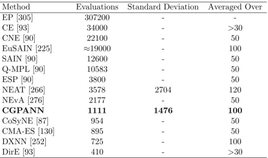
9.4 Applying CGPANN to Classification . . . 210 9.5 Comparative Methods . . . 212 9.6 Benchmarks . . . 214 9.7 Results . . . 215 9.8 Discussion . . . 217 9.9 Summary . . . 219
10 Recurrent CGPANN Applied to Series Forecasting 221 10.1 Structure of this Chapter . . . 221
10.2 Background . . . 222
10.3 Recurrent CGPANN . . . 223
10.4 Applying CGP, RCGP, CGPANN and RCGPANN to Series Forecasting . . 224
10.5 Comparative Methods . . . 226
10.6 Results . . . 228
10.7 Discussion . . . 239
10.8 Summary . . . 241
11 Conclusions and Further Work 243 11.1 Structure of this Chapter . . . 243
11.2 Overall Conclusions . . . 243
11.3 Further Work . . . 250
11.4 Final Remarks . . . 259
Appendix 261 A Benchmarks 261 A.1 Structure of this Appendix . . . 261
A.2 Control . . . 261
A.3 Classification . . . 266
A.4 Boolean Circuits . . . 271
A.5 Symbolic Regression . . . 272
A.6 Forecasting . . . 275
B Statistical Significance Testing 279 B.1 Structure of this Appendix . . . 279
B.2 Background . . . 279
B.3 Distribution of Evolutionary Algorithm Results . . . 280
B.4 Non-Parametric Statistical Significance Testing . . . 281
C Cartesian Genetic Programming Library 283 C.1 Structure of this Appendix . . . 283
C.2 Background . . . 283 C.3 Overall Functionality . . . 284 C.4 Visualisation . . . 286 C.5 NeuroEvolution . . . 287 C.6 Recurrent Networks . . . 288 C.7 Licenses . . . 288
C.8 Using the CGP Library . . . 288
C.9 Discussion . . . 289
List of Figures
2.1 Simple depiction of a biological neuron taken fromwww.newworldencyclopedia. org. . . 9 2.2 Simple generalised model of an artificial neuron. . . 11 2.3 Common non-spiking neuron models. . . 13 2.4 Example of data which is linearly separable (a) and the XOR gate which is
not linearly separable (b). . . 14 2.5 Zero hidden layer feed-forward neural network with four inputs and one
output. . . 14 2.6 Simple ANN comprising two inputs, one hidden layer containing three
neu-rons, and one output neuron. . . 16 2.7 Example of a SANE individual showing that each neuron describes the
inputs and outputs to which it connects and the corresponding connection weights. . . 32 2.8 Example Cellular Encoding developmental operations. (a) gives an initial
network. (b) gives an example of parallel cell division; where the mother cell is replaced (divided) into two identical cells. (b) gives an example of sequential cell division; where the mother cell is replaced (divided) into two cells with the first taking the mother cells inputs, the second taking the mother cells outputs. . . 36 2.9 An example NEAT genotype and its decoded phenotype. . . 37 2.10 Example of HyperNEAT. The first network, constructed using NEAT, is
used to assign the weights in the second based on the positions of the two connected nodes. Here only connections between layers are shown but typically connections between all possible nodes would be evaluated. . . 38 2.11 An example of a GNARL ANN. . . 40 2.12 EANT Genotype Phenotype mapping, taken from [143]. The Genotype (a)
is decoded as a tree from root to leaves. N gives the node to connect to and I the input. J F and J R stand for feed forward and recurrent jumper connections respectively and are added to the tree by assuming they increase the arity of the current node. The corresponding phenotype is given in (b). 44 2.13 NevA Genotype Phenotype mapping, taken from [276] . . . 45 3.1 Example CGP program with three inputs, three available nodes and two
outputs. The active genes are shown in bold with the inactive in grey. The corresponding chromosome is as follows: 012 233 104 3 4 . . . 58 3.2 Generalised depiction of the original rows and columns form of a CGP
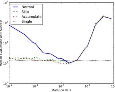
chromosome; shown graphically above and as a string below. Image taken from [202] . . . 59 3.3 Comparison of various mutation methods on the 3 Bit Even Parity
4.1 Example CGPANN program with three inputs, three available nodes and
two outputs. . . 76
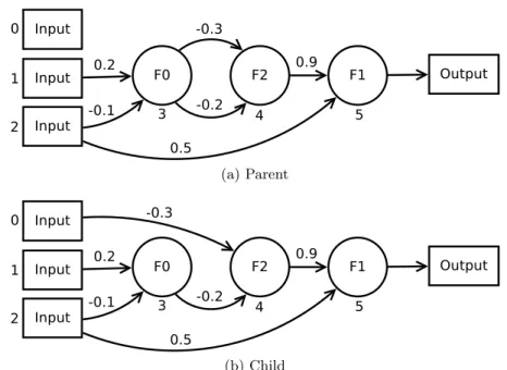
4.2 Small topology mutation. The parent chromosome (a) has had a single topology mutation resulting in a child (b) where node 4 is now connected to input 0. All other nodes are left unchanged. . . 79
4.3 Large topology mutation. The parent chromosome (a) has had a single topology mutation resulting in a child (b) where the output is now connected to input 0. All other nodes are now unused. . . 79
4.4 Depiction that multiple inter-node connections (a) is equivalent to one con-nection with the sum of the individual concon-nection weights (b). . . 91
4.5 The bloat metric comparing standard tree-based GP (light gray) and DynOpEq GP (black) on (a) symbolic regression and (b)(c) two real world classifica-tion tasks. Images taken from [284]. . . 95
4.6 Average fitness, number of active nodes and program bloat Vs. generation for CGP applied to the six bit even parity benchmark. . . 97
4.7 Average fitness, number of active nodes and program bloat Vs. generation for CGP applied to the Pagie 1 benchmark. . . 98
4.8 Average fitness, number of active nodes and program bloat Vs. generation for CGPANN applied to the double pole benchmark. . . 100
4.9 Average fitness, number of active nodes and program bloat Vs. generation for CGPANN applied to the ball throwing benchmark. . . 101
4.10 Average fitness, number of active nodes and program bloat Vs. generation for CGPANN applied to the Monks Problem 1 benchmark. . . 102
5.1 Example RCGP program corresponding to the chromosome: 212 005 134 5 107 5.2 Example RCGP program corresponding to the chromosome: 002 055 144 5 109 5.3 Depiction of the “Santa Fe Ant Trail”. Black and white represents food and no food respectively. . . 112
5.4 Number of yearly recorded sunspots between 1700 and 1987. . . 113
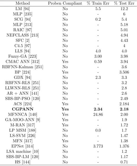
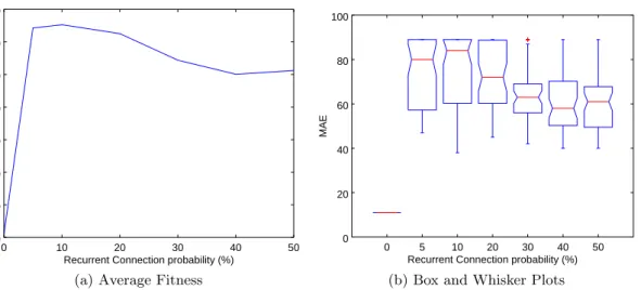
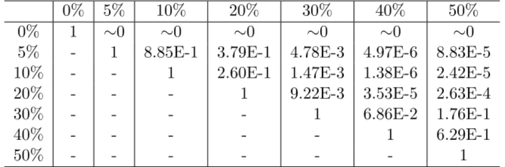
5.5 Results of varying RCGP’s recurrent connection probability on the Artificial Ant benchmark. . . 114
5.6 Results of varying RCGP’s recurrent connection probability on the Sunspots benchmark: training data. . . 116
5.7 Results of varying RCGP’s recurrent connection probability on the Sunspots benchmark: testing data. . . 116
5.8 Number sequences shown graphically. . . 120
5.9 Example CGP (a) and RCGP (b) Hexagonal solutions. . . 121
5.10 Example RCGP Lazy Caterer solutions. . . 121
5.11 Example CGP (a) and RCGP (b) Magic Constants solutions. . . 122
5.12 Example RCGP Fibonacci solution. . . 122
6.1 Effect of sweeping topology and topology limits for CNE and CGPANN respectively. . . 134
6.2 MLP trained using resilient back propagation on the Monks Problem. Note the larger range of finesses than displayed in Figure 6.1. . . 135
6.3 Solution found by CGPANN for the Double Pole Balancing benchmark. . . 137
6.4 Comparing the relative importance of connection weight evolution and topology evolution using CGPANN on the Ball Throwing benchmark. . . . 140 6.5 Comparing the relative importance of connection weight evolution and
6.6 Comparing the relative importance of connection weight evolution and topology evolution using CGPANN on the Monks Problem 1 benchmark. . 141 7.1 Heaviside step function (a), Gaussian function (b) and the logistic sigmoid
function (c). Withσ= 1 for the Gaussian and logistic functions. . . 151 7.2 Variable Gaussian function. . . 151 7.3 Variable logistic sigmoid function. . . 151 7.4 Fitnesses achieved from applying CNE to the Ball Throwing benchmark. . . 164 7.5 Generations required from applying CNE to the Ball Throwing benchmark. 164 7.6 Fitnesses achieved in applying CNE to the Full Adder benchmark. . . 165 7.7 Generations required from applying CNE to the Full Adder benchmark. . . 165 7.8 Fitnesses achieved in applying CNE to the Monks Problem 1 benchmark
-Training. . . 165 7.9 Fitnesses achieved in applying CNE to the Monks Problem 1 benchmark
-Testing. . . 165 7.10 Fitnesses achieved in applying CNE to the Two Spirals benchmark. . . 166 7.11 Fitnesses achieved in applying CNE to the Proben Cancer1 benchmark
-Training. . . 166 7.12 Fitnesses achieved in applying CNE to the Proben Cancer1 benchmark
-Testing. . . 166 7.13 Fitnesses achieved in applying CGPANN to the Ball Throwing benchmark. 166 7.14 Generations required from applying CGPANN to the Ball Throwing
bench-mark. . . 167 7.15 Fitnesses achieved in applying CGPANN to the Full Adder benchmark. . . 167 7.16 Generations required from applying CGPANN to the Full Adder benchmark.167 7.17 Fitnesses achieved in applying CGPANN to the Monks Problem 1
bench-mark - Training. . . 167 7.18 Fitnesses achieved in applying CGPANN to the Monks Problem 1
bench-mark - Testing. . . 168 7.19 Fitnesses achieved in applying CGPANN to the Two Spirals benchmark. . . 168 7.20 Fitnesses achieved in applying CGPANN to the Proben Cancer1 benchmark
- Training. . . 168 7.21 Fitnesses achieved in applying CGPANN to the Proben Cancer1 benchmark
- Training. . . 168 8.1 Implicit genetic redundancy in tree-based GP. Active nodes are shown in
black, implicitly redundant nodes in grey. . . 175 8.2 Example of ENGD occurring with a fitness improvement. Active genes are
given in bold, explicitly inactive in grey and implicitly inactive in dashed. . 183 8.3 Example of ENGD occurring without a fitness improvement. Active genes
are given in bold, explicitly inactive in grey and implicitly inactive in dashed.184 8.4 Example of INGD occurring with a fitness improvement. Active genes are
given in bold, explicitly inactive in grey and implicitly inactive in dashed. . 184 8.5 Example of INGD occurring without a fitness improvement. Active genes
are given in bold, explicitly inactive in grey and implicitly inactive in dashed.185 8.6 Number of available nodes versus fitness and percentage of active nodes. . . 194 9.1 Results given in Table 9.1, presented as bar charts. . . 216 10.1 Depiction of recurrent forecasting and the use of embedding dimension and
10.2 Spread of the forecasts produced using stochastic methods on the Laser
benchmark. . . 232
10.3 Spread of the forecasts produced using stochastic methods on the Mackey Glass benchmark. . . 234
10.4 Spread of the forecasts produced using stochastic methods on the Sunspots benchmark. . . 236
10.5 Laser forecasts produced using the various forecasting methods. . . 236
10.6 Mackey Glass forecasts produced using the various forecasting methods. . . 237
10.7 Sunspots forecasts produced using the various forecasting methods. . . 238
11.1 Depiction of length bias in CGP. Generated by applying CGP to a flat fitness landscape. Image taken from [82] . . . 251
11.2 Results from applying RCGPANN to the configuration of the reservoir to be used by reservoir computing. . . 253
A.1 Depiction of the single pole balancing benchmark. . . 262
A.2 Depiction of the double pole balancing benchmark. . . 262
A.3 Depiction of the ball throwing benchmark. . . 265
A.4 Depiction of the Two Spiral Classification benchmark. . . 271
A.5 Nguyen 10 . . . 273
A.6 Pagie . . . 274
A.7 Tower Problem . . . 274
A.8 Laser series forecasting benchmarks. . . 276
A.9 Mackey-Glass series forecasting benchmarks. . . 277
A.10 Sunspot series forecasting benchmarks. . . 277
B.1 Histogram of 1000 runs showing the number of generations required for CGP to find a solution to the full adder task. . . 281
B.2 Depiction of the effect size measure. (a) shows two distribution which would be awarded a smaller effect size and (b) a larger. . . 282
List of Tables
2.1 Taxonomy of NeuroEvolutionary methods . . . 46
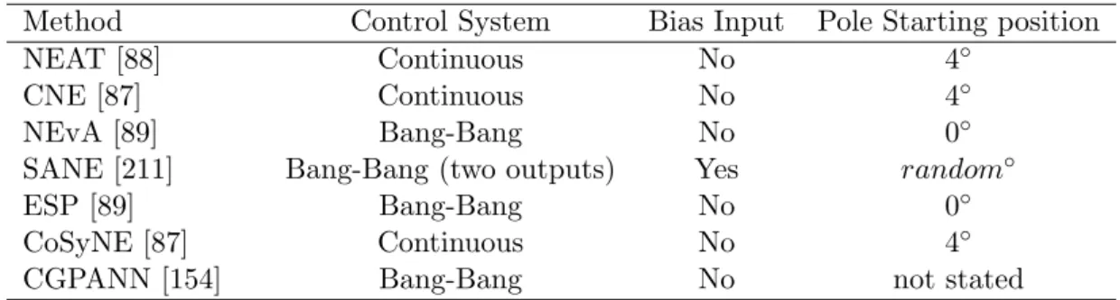
2.2 Differences in the single pole benchmark implementations used in the Neu-roEvolutionary literature. . . 53
3.1 Standard parameters used by CGP. . . 63
4.1 Comparison of results for the Double Pole Balancing benchmark . . . 87
4.2 Comparison of results for the Ball Throwing benchmark . . . 88
4.3 Comparison of results for the Proben 1: Cancer 1 benchmark . . . 89
4.4 Applying CGPANN to a range of benchmarks with and without the use of connection switch (CS) genes. The best performance is given in bold. Statistical significance is also give with p < 0.05 given in bold. The effect size is also given. . . 93
5.1 Artificial Ant: pvalues comparing pairs of recurrent connection probabilities.115 5.2 Sunspots training fitness: p values comparing pairs of recurrent connection probabilities. . . 116
5.3 Sunspots testing fitness: p values comparing pairs of recurrent connection probabilities. . . 117
5.4 Performance of CGP and RCGP finding explicit and recurrent equations respectively which produce famous mathematical sequences. In each case the average number of evaluations is given followed by the number of runs which successfully solved the task in brackets. . . 120
5.5 GP methods applied to the Fibonacci Sequence benchmark . . . 123
6.1 Statistical analysis of the relative importance of connection weight evolution and topology evolution on the Ball Throwing benchmark. . . 142
6.2 Statistical analysis of the relative importance of connection weight evolution and topology evolution on the Double Pole benchmark. . . 142
6.3 Statistical analysis of the relative importance of connection weight evolution and topology evolution on the Monks Problem 1 benchmark. . . 142
7.1 Fitness achieved using homogeneous ANNs of different TFs trained using CNE. . . 154
7.2 Number of generations required to find optimal solutions using homoge-neous ANNs of different TFs trained using CNE. . . 154
7.3 fitness achieved using homogeneous ANNs of different TFs trained using CGPANN. . . 154
7.4 Number of generations required to find optimal solutions using homoge-neous ANNs of different TFs trained using CGPANN. . . 154
7.5 Statistical significance between the homogeneous CNE fitness results given in Table 7.1. . . 154 7.6 Statistical significance between the homogeneous CNE generational results
given in Table 7.2. . . 155 7.7 Statistical significance between the homogeneous CGPANN fitness results
given in Table 7.3. . . 155 7.8 Statistical significance between the homogeneous CGPANN generational
results given in Table 7.4. . . 155 7.9 Effect Size between the homogeneous CNE fitness results given in Table 7.1. 155 7.10 Effect Size between the homogeneous CNE generational results given in
Table 7.2. . . 155 7.11 Effect Size between the homogeneous CGPANN fitness results given in
Ta-ble 7.3. . . 156 7.12 Effect Size between the homogeneous CGPANN generational results given
in Table 7.4. . . 156 7.13 Average results achieved using heterogeneous ANNs trained using CNE.
The result is given in bold if evolving heterogeneous ANNs outperformed the average fitness of using each transfer function individually. . . 158 7.14 Average results achieved using heterogeneous ANNs trained using
CG-PANN. The result is given in bold if evolving heterogeneous ANNs out-performed the average fitness of using each transfer function individually. . 158 7.15 Average fitness of ANNs of variable Gaussian TFs trained using CNE. . . . 159 7.16 Average number of generations required to find optimal solutions using
ANNs of variable Gaussian TFs trained using CNE. . . 160 7.17 Average fitness of ANNs of variable logistic TFs trained using CNE. . . 160 7.18 Average number of generations required to find optimal solutions using
ANNs of variable logistic TFs trained using CNE. . . 160 7.19 Average fitness of ANNs of variable Gaussian TFs trained using CGPANN. 160 7.20 Average number of generations required to find optimal solutions using
ANNs of variable Gaussian TFs trained using CGPANN. . . 160 7.21 Average fitness of ANNs of variable logistic TFs trained using CGPANN. . 160 7.22 Average number of generations required to find optimal solutions using
ANNs of variable logistic TFs trained using CGPANN. . . 161 7.23 Average fitness of variable heterogeneous ANNs trained using CNE. . . 163 7.24 Average number of generations required to find optimal solutions using
variable heterogeneous ANNs trained using CNE. . . 163 7.25 Average fitness of variable heterogeneous ANNs trained using CGPANN. . . 163 7.26 Average number of generations required to find optimal solutions using
variable heterogeneous ANNs trained using CGPANN. . . 163 8.1 Restrictions made to CGP used in order to investigate NGD. . . 186 8.2 Comparing regular CGP to only mutating active genes in order to isolate
the benefit of ENGD. In all cases a lower fitness represents a better search. 187 8.3 Comparing regular CGP to only selecting fitness improvements in order to
isolate the benefit of NGD and other forms of redundancy aiding the escape from local optima. In all cases a lower fitness represents a better search. . . 188 8.4 Selecting only fitness improvements compared with only allowing mutations
to active genes while also only selecting fitness improvements. This isolates the benefits of ENGD other than aiding the escape of local optima. In all cases a lower fitness represents a better search. . . 189
8.5 Number of available nodes which resulted in the lowest errors presented in Figure 8.6. . . 195 8.6 Comparing regular CGPANN to only mutating active genes in order to
isolate the benefit of ENGD. In all cases a lower fitness represents a better search. . . 198 8.7 Comparing regular CGPANN to only mutating active genes in order to
isolate the benefit of ENGD. In all cases a lower number of generations represents a better search. . . 198 8.8 Comparing regular CGPANN to only selecting fitness improvements in
or-der to isolate the benefit of NGD aiding the escape from local optima. In all cases a lower fitness represents a better search. . . 199 8.9 Comparing regular CGPANN to only selecting fitness improvements in
or-der to isolate the benefit of NGD aiding the escape from local optima. In all cases a lower number of generations represents a better search. . . 199 8.10 Selecting only fitness improvements compared with only allowing mutations
to active genes while only selecting fitness improvements. This isolates the benefits of ENGD other than aiding the escape of local optima. In all cases a lower fitness represents a better search. . . 200 8.11 Selecting only fitness improvements compared with only allowing mutations
to active genes while only selecting fitness improvements. This isolates the benefits of ENGD other than aiding the escape of local optima. In all cases a lower number of generations represents a better search. . . 200 8.12 Percentage of active nodes used by CGP and CGPANN. . . 201 8.13 Comparing regular CGPANN using an increased number of available nodes
to only mutating active genes in order to isolate the benefit of ENGD. In all cases a lower fitness represents a better search. . . 202 8.14 Comparing regular CGPANN using an increased number of available nodes
to only mutating active genes in order to isolate the benefit of ENGD. In all cases a lower number of generations represents a better search. . . 202 9.1 Classification accuracy of a range of classification methods. . . 215 9.2 Closer Comparison of MLPs and CGPANN . . . 217 9.3 Previously presented classification performance of standard classification
algorithms and CGPANN on the breast cancer benchmark. . . 218 10.1 Parameters by CGP and its derivatives. . . 226 10.2 Results from applying various forecasting methods to the Laser benchmark. 231 10.3 Statistical significance testing between the stochastic methods applied to
the Laser benchmark. . . 231 10.4 Results from applying various forecasting methods to the Mackey-Glass
benchmark. . . 233 10.5 Statistical significance testing between stochastic methods on the
Mackey-Glass benchmark. . . 233 10.6 Results from applying various forecasting methods to the Sunspots
bench-mark. . . 235 10.7 Statistical significance testing between stochastic methods on the Sunspots
benchmark. . . 235 A.1 Pole balancing symbol definitions and commonly used values. . . 263 A.2 Ball throwing symbol definitions and commonly used constants. . . 265
A.3 Monks Problem Robot Appearances. . . 270 C.1 Example CGP chromosome displayed using printChromosome. . . 286
Acknowledgements
I would like to acknowledge the funding provided by the EPSRC, without which this thesis would not have been possible. I am pleased to live in a country which both values and supports academic research.
The experience of undertaking a PhD is strongly determined by the relationship be-tween the student and their supervisor. In this regard I consider myself highly fortunate. Julian has not only been an exceptional supervisor, but also a mentor. He has given academic, and life advice. I am wholly grateful for his time and company, both in a supervisory setting, and in the early hours at conference hotel bars.
There are two particular friends which have been quintessential to my PhD experience. Nils Morozs and Stuart Lacy, we will graduate from York not once, but twice together. I wish you both great success.
I will be forever grateful to my Mum, Dad and Brother, my family. I don’t know their initial feelings when I turned down a “proper job” to perpetuate my life as a student, but they have shown nothing but loving support. I have the utmost pride in my family, and feel fulfilled in the pride they have for me.
Katherine, we share a life here in York which I hope will never end. We love, support and amuse each other as we ramble through life day to day. I can’t wait to see where our ramblings take us next together.
Declaration
I declare that the research described in this thesis is original work, which I undertook at the University of York during 2012 - 2015. This work has not previously been presented for an award at this, or any other, University.
Some parts of this thesis have been published in journals and conference proceedings; where items were published jointly with collaborators, the author of this thesis is respon-sible for the material presented here. For each published item the primary author is the first listed author.
Journal Articles and Letters
• Turner, A. J. & Miller, J. F. Introducing A Cross Platform Open Source Cartesian Genetic Programming Library. In Genetic Programming and Evolvable Machines, vol 16, pages 83-91, 2014.
• Turner, A. J. & Miller, J. F. NeuroEvolution: Evolving Heterogeneous Artificial Neural Networks. InEvolutionary Intelligence, vol 7, pages 135-154, 2014.
• Turner, A. J. & Miller, J. F. Neutral Genetic Drift: an Investigation using Cartesian Genetic Programming. InGenetic Programming and Evolvable Machines, 2015.
Conference Proceedings
• Turner, A. J. & Miller, J. F. Cartesian Genetic Programming encoded Artificial Neural Networks: A Comparison using Three Benchmarks. In Proceedings of the Conference on Genetic and Evolutionary Computation (GECCO-13), pages 1005-1012, 2013.
• Turner, A. J. & Miller, J. F. The Importance of Topology Evolution in NeuroEvo-lution: A Case Study Using Cartesian Genetic Programming of Artificial Neural Networks. In Research and Development in Intelligent Systems XXX, pages 213-226, 2013.
• Turner, A. J. & Miller, J. F. Cartesian Genetic Programming: Why No Bloat?. In
Genetic Programming: 17th European Conference (EuroGP-2014), pages 193-204, 2014.
Evolution and Heterogeneous Networks. In Proceedings of the 50th Anniversary Convention of the AISB, pages 158-165, 2014.
• Turner, A. J. & Miller, J. F. Recurrent Cartesian Genetic Programming. In 13th International Conference on Parallel Problem Solving from Nature (PPSN 2014), pages 476-486, 2014.
• Turner, A. J. & Miller, J. F. Recurrent Cartesian Genetic Programming Applied to Famous Mathematical Sequences. In Proceedings of the Seventh York Doctoral Symposium on Computer Science & Electronics (YDS 2014), pages 37-46, 2014. • Turner, A. J. & Miller, J. F. Recurrent Cartesian Genetic Programming Applied
to Series Forecasting. In Proceedings of the Genetic and Evolutionary Computation Conference (GECCO-15), pages 1499-1500, 2015.
Introduction
This chapter provides an overview of the thesis, presenting the motivation and aims of the work, the main contributions made and a summary of the chapters presented.
1.1
Structure of this Chapter
Section 1.2 provides high level motivation for the work presented throughout this thesis. Section 1.3 gives the high level aims of the thesis. Section 1.4 describes the significant contributions which have been made during the thesis. Finally, Section 1.5 gives an outline of the remaining chapters and appendixes.
1.2
Motivation
Artificial Neural Network (ANN)s and Evolutionary Algorithm (EA)s represent two pow-erful, widely adopted, machine learning methodologies strongly inspired by biological sys-tems. However, there is one important distinction between ANNs and EAs. ANNs repre-sent an abstraction of biological brains which must be trained (optimised) in order to solve a given task. Whereas EAs are an optimisation method based on Darwinian Evolution. Interestingly, this means that these two, independent, machine learning methods can be combined by using EAs to optimise the configuration of ANNs. This union of ANNs and EAs is termed NeuroEvolution (NE).
The combination of EAs and ANNs is not just of academic interest but is thought to provide a number of significant advantages over many other ANN training methods. For instance, NE can easily be applied to the creation of feed-forward and recurrent networks,
it can be used to apply ANNs to supervision and reinforcement learning tasks, the depth of the network has no influence on the learning algorithm, it can be used to evolve networks of heterogeneous neuron transfer functions, and finally, it can be used to adapt both connection weights as well as the network topology.
Despite the increasing popularity of NE methods, there are a number of significant gaps in the literature; notably those concerning the perceived benefits of NE. For example, it is often stated that one of the major advantages of NE is its ability to determine network topology. However, there is surprisingly little empirical research which assess whether, and to what extent, evolving network topology actually provides an advantage. Additionally, it is often stated that the ability for NE to create heterogeneous ANNs represents an advantageous characteristic. However, as with topology configuration, there is currently very little empirical evidence to support this.
There are also highly significant topics within the field of EAs that are mostly absent in the field of NE. For instance, issues concerning program bloat and the effect of genetic redundancy are almost never considered.
Therefore, if the field of NE is to progress, these gaps in the literature must be ad-dressed. This represents one of the key motivations of this work.
The second motivation is concerned with developing further the technique of Cartesian Genetic Programming of Artificial Neural Networks (CGPANN), a recently developed NE method created by Maryam Mahsal Khan et al. in 2010. CGPANN is a NE method based on Cartesian Genetic Programming (CGP). CGP is a graph based form of Genetic Pro-gramming (GP) which is uniquely suited to describing ANNs; due to it encoding general directed feed-forward Multiple-Input Multiple-Output (MIMO) graphs of computational elements. The only alterations required to apply CGP to the evolution of ANNs is the addition of connection weights and the use of transfer functions typically associated with ANNs. Additionally, CGP is an established GP method which has undergone much de-velopment and theoretical study. A large proportion of this previous work applies directly to CGPANN and therefore provides many possibilities for future ANN developments.
1.3
Thesis Aims
Based on the described motivations, and material presented in the literature review, a number of thesis aims are proposed.
1. To investigate whether the ability to adapt network topology represents an advan-tageous property of NeuroEvolution.
2. To investigate whether the ability to create heterogeneous Artificial Neural Networks represents an advantageous property of NeuroEvolution.
3. To extend the Cartesian Genetic Programming algorithm to be capable of creating recurrent program structures.
4. To apply the developed recurrent Cartesian Genetic Programming extension to the evolution of recurrent Artificial Neural Networks.
5. To investigate the role of genetic redundancy on Cartesian Genetic Programming’s evolutionary search; with a focus on its application to training Artificial Neural Networks.
6. To investigate the suitability of applying Cartesian Genetic Programming as a train-ing method for Artificial Neural Networks in the domains of classification and series forecasting.
1.4
Thesis Contributions
Throughout this thesis a number of substantial contributions are made to CGP, CGPANN and the wider field of NE. The most significant contributions are now summarised.
1. This thesis presents Recurrent Cartesian Genetic Programming (RCGP), a signifi-cant CGP extension which enables the creation of both acyclic and cyclic program structures. In this thesis RCGP is shown to be capable of solving tasks intractable to standard CGP. Additionally, when applied to series forecasting, RCGP is demon-strated to not only outperform standard CGP, but also a range of popular standard forecasting methods.
2. This thesis presents the application of the RCGP extension to CGPANN in order to facilitate the evolution of Recurrent Artificial Neural Network (RANN)s. This recur-rent CGPANN extension is termed Recurrecur-rent Cartesian Genetic Programming of Ar-tificial Neural Networks (RCGPANN). As with RCGP, RCGPANN is demonstrated to be a highly effective forecasting method outperforming all standard forecasting methods used for comparison.
3. A significant proportion of this thesis is dedicated to providing rigorous empirical evidence of many of the perceived advantages of NE. This has been achieved for two domains. Firstly, it has been show that the ability for many NE methods to evolve the network topology, as well as connection weights, of ANNs represents a significant advantage over training methods which only optimise connections weights. Results presented indicate that the importance of topology optimisation may even be more significant to training than connection weight optimisation. Secondly, it has been shown that the ability of nearly all NE methods to create heterogeneous ANNs represents a significant, and widely overlooked, advantage over training methods which solely train homogeneous ANNs.
4. This thesis rigorously, and extensively, evaluates the role and benefit of genetic redundancy in both CGP and CGPANN. It is shown that the presence of genetic redundancy in CGP provides a substantial advantage to the evolutionary search; primarily through its ability to aid the escape of local optima in the search space. It is also shown that the benefit of genetic redundancy is substantially lower when evolving ANNs. Theoretical explanations of this interesting discrepancy between CGP and CGPANN are provided based on the influence of connection weights on the search.
5. This thesis rigorously assesses CGPANN in the domains of classification and series forecasting. In both cases the studies go beyond previous applications of CGPANN in terms of the methodology, the range of benchmark problems employed and the number of methods used for comparison. From these applications it is demonstrated that CGPANN performs poorly in the domain of classification and exceptionally well in the domain of series forecasting.
6. Finally, during this thesis an open source cross platform CGP library was developed. This library provides a stable, tested, implementation of CGP along with all of
the extensions and developments made during this thesis: RCGP, CGPANN and RCGPANN. This contribution is significant for two main reasons. Firstly, it allows others to learn, use, research and apply all of the developments made in this thesis. Secondly, it allows the presented experiments to be able to be replicated by others.
1.5
Thesis Outline
This section outlines the remaining chapters of this thesis.
Chapter 2 provides an introduction to NE in general, including descriptions of the more popular NE methods. A substantial review of the NE literature is also undertaken with the insights gained used to guide the research presented.
Chapter 3 provides a detailed description of CGP, the underlying algorithm of the NE method of interest in this thesis; CGPANN. This description includes the basic algo-rithm, distinguishing features, a summary of common applications and a discussion of the extensions and theoretical work which have been developed.
Chapter 4describes CGPANN, the NE method of interest in this thesis. This chap-ter describes the CGPANN implementation, possible advantages over other NE methods and previous applications. Additionally, a number of experiments are presented applying CGPANN to standard benchmark problems, assessing previous design decisions made for CGPANN and demonstrating that CGPANN, like CGP, is immune to program bloat.
Chapter 5presents a new extension made to the CGP algorithm in order to enable the encoding of cyclic program structures. This new method is termedRecurrent Cartesian Genetic Programming and represents a superset of CGP; capable of evolving both recur-rent and feed-forward program structures. The chapter also presents a number of initial experiments demonstrating that RCGP is indeed capable of evolving cyclic programs.
Chapter 6presents a number of experiments demonstrating the advantages of evolv-ing ANN topology. This work fills a current gap in the literature where it is often assumed that evolving ANN topology represents an advantageous property, with little empirical evidence to support the claim.
Chapter 7 presents a number of experiments demonstrating the advantages of using NE to evolve heterogeneous ANNs. Despite many calls in the literature for research in this area, very little work has been previously presented which assesses the benefit of evolving heterogeneous ANNs. This work addresses this gap in the literature.
drift for both CGP and CGPANN. The work demonstrates that CGP greatly benefits from the increased genetic redundancy provided by its encoding. The work also identifies that CGPANN benefits significantly less from neutral genetic drift than CGP, despite being based on the same underlying algorithm.
Chapter 9presents a rigorous evaluation of CGPANN in the domain of classification. The work demonstrates that CGPANN performs poorly compared to a range of standard classification techniques.
Chapter 10 presents a rigorous evaluation of RCGPANN in the domain of series forecasting where it is shown to outperform all standard forecasting techniques used for comparison. Additionally, CGP, RCGP and CGPANN are applied to the same tasks in order to assess which aspects of RCGPANN contribute to its strong performance; the recurrent extension or the application to ANNs.
Chapter 11gives the final overall conclusions of the thesis along with proposed future work.
Appendix A describes, in detail, the benchmarks which are used throughout this thesis.
Appendix Bdescribes, and justifies, the statistical significance testing methods used when analysing the empirical investigations undertaken in this thesis.
Appendix C describes an open source cross platforms CGP implementation which was developed during the PhD program.
NeuroEvolution
NeuroEvolution (NE) [64,112,313] is a sub field of Machine Learning (ML) which combines both Evolutionary Algorithm (EA)s and Artificial Neural Network (ANN)s. This chapter introduces the field of NE with a focus on the more popular NE methods. This is followed by a review of the wider NE literature which is used to guide the research presented throughout this thesis.
2.1
Structure of this Chapter
Section 2.2 introduces the basic principles concerning NE along with a description of a simplistic NE method. Section 2.3 describes a number of advantageous properties of NE over other ANN training methods. Section 2.4 discusses the scope of NE in terms of which aspects of ANNs it can be used to optimise. Section 2.5 describes a range encoding schemes used by NE to describe ANNs. Section 2.6 provides a detailed review of many popular NE methods. Section 2.7 presents a detailed literature review of the general field of NE. Finally, Section 2.8 gives a closing discussion of the chapter.
2.2
Basic Principles
NE is the application of EAs to the training of ANNs. Therefore a brief introduction of both EAs and ANNs is provided. This is followed by a description of using a simple Genetic Algorithm (GA), a type of EA, as an ANN training method. This summary of the basic principles surrounding NE is intended to act as a reminder to those already familiar with the field, and to focus on concepts which will be relevant later in the thesis.
2.2.1 Evolutionary Algorithms
EAs [72, 228] represent a family of stochastic1, heuristic2 population based3 search tech-niques based on Darwinian evolution [49]4.
EAs are initialised by creating a population of random solutions to a given problem encoded in what are termed chromosomes or genotypes; taking the terminology from the biology from which they are inspired. Each of the chromosomes are then decoded into their corresponding solutions, termed phenotypes, and assigned a fitness value propor-tional to their effectiveness at solving the given task. The fitness of each chromosome is then used to determine which are selected, mimicking the concept of “survival of the fittest” or “natural selection”. The selected chromosomes are then used as parents in the creation of new child chromosomes; the unselected chromosomes are discarded. Child chromosomes can be created from their parents via asexual or sexual reproduction. In the asexual case, the created children are clones of the parents with random alterations applied; these alterations are termed mutations again using biological terminology. In the sexual case, the child chromosomes contain genetic material from two or more of the parent chromosomes; mutation can then also be applied. This next generation of chromosomes is then comprised of the newly created child chromosomes; with or without the selected parents. This process of assigning fitness, selection and reproduction is then repeated until a termination condition is reached. Typical termination conditions specify a maximum number of generations and a target fitness value i.e. when a solution is found which is considered satisfactory. The entire process is shown in Algorithm 1.
Algorithm 1 Basic Evolutionary Algorithm Initialise a population of random chromosomes
whileTermination Conditions not met do
Calculate chromosome fitness
Select chromosomes for reproduction Reproduce via mutation and/or crossover
end while
1Involves a random element in the search process. 2
Uses experience and/or learning to guide the search.
3Makes used of many agents working together or independently. 4
The creation of EAs is attributed to the contributions of three groups who indepen-dently conducted research in the area unaware of each other’s work. Each of their works is now considered a separate sub-field of EAs called: Evolutionary Programming (EP) [67], GAs [113] and Evolutionary Strategies (ES) [237]. Interestingly however, the notion of us-ing artificial evolution as a problem solvus-ing tool was also proposed by Alan Turus-ing in 1948 (long before the other discoveries), his essay was dismissed by his employer, the grandson of Charles Darwin, as a “schoolboy essay” [277]. For a more detailed and complete history of EAs see [66].
2.2.2 Artificial Neural Networks
Like EAs, ANNs are also heavily inspired by biology and represent, to a greater or lesser extent, a simplified abstraction of real neural networks found within the brains of animals. ANNs comprise a weighted directed acyclic/cyclic graph where each node implements a transfer function which approximates a biological neuron.
Biological neurons5 take the form of that shown in Figure 2.1. Each neuron gathers at its dendrites (inputs) signals from other neuron’s axons (outputs). These input signals propagate along the dendrites down into the soma (cell body). These signals cause the membrane potential of the neuron to increase or decrease depending upon whether the signal is excitatory or inhibitory respectively. If the membrane potential reaches a certain upper threshold, the neuron fires, propagating a signal down its own axon and out to other neurons; otherwise no output signal is produced.
Figure 2.1: Simple depiction of a biological neuron taken from www. newworldencyclopedia.org
5The existence of neurons was first discovered by Santiago Ram´on y Cajal the late 19thcentury which resulted in him receiving a noble prize for his contributions
Signals are passed between neurons, from axons to dendrites, at synaptic connec-tions. Synapses are the junctions between axon terminals and dendrites. They release a neurotransmitter when excited by a signal from the axon. This neurotransmitter then propagates across the gap between axon terminal and dendrite (synaptic cleft) causing a signal to be induced in the dendrite. The magnitude of this signal is proportional to the connection strength of the synapse. This signal is excitatory or inhibitory depending on the type of synapse between axon and dendrite.
In biological neural networks the signals passed between neurons are spikes of poten-tial difference between the ions internal and external to the neuron. ANNs which model this spiking behaviour are referred to as Spiking Neural Networks (SNN). Neuron mod-els commonly used by SNN include the Hodgkin-Huxley model6 [111], integrate and fire
model7 [1] and the Izhikevich neuron model [131].
However, the majority of NE methods, and ANN training methods in general, construct ANNs consisting of spiking neuron models. This is most likely because simulating non-spiking ANNs is much less computationally expensive whilst being powerful enough to be applied to many applications. Non-spiking neuron models do however contain many of the characteristics of their spiking counterparts. Their output is determined by their inputs and the strength of the connection weights (synapse connections). Additionally, although the signals passed between neurons are not actually spikes, they can be thought of as an abstraction of this concept. For instance, if a neuron outputs 0 or 1, 1 can be considered spiking and a 0 can be considered not spiking. Alternatively, if a neuron outputs a floating point value in the range [0,1], this can be considered as a spiking (firing) rate; with zero being no spikes, 0.5 being alternating spikes and no spikes, and 1.0 being continuous spiking.
Nearly all non-spiking neuron models can be generalised to the model shown in Figure 2.2. The inputsxi are the inputs from previous neurons, the weightswiare the connection
strengths of the synapses, the functionϕ() describes the transfer function (internal logic) of the neuron, the biasbis used for any internal thresholds, and the outputyis the output of the neuron provided byϕ().
Non-spiking neuron transfer functions are typically a function of the weighted sum of
6The implementation of the Hodgkin-Huxley neuron model was so significant that it resulted in Alan Lloyd Hodgkin and Andrew Huxley receiving the Nobel Prise in Physiology or Medicine in 1963.
7Interestingly the integrate and fire neuron model was developed by Louis Lapicque in 1907 [1], long before the mechanics of biological neurons were understood.
Figure 2.2: Simple generalised model of an artificial neuron.
inputs. The weighted sum of inputs S is equivalent to the dot product of the neuron’s inputs as a vector X and the neuron’s connection weight as a vector W, as shown in equation 2.1. The transfer function of a non-spiking neural model usually takes the form of Equation 2.2, whereϕ() changes from model to model.
S =W ·X= n X i=0 wixi (2.1) y=ϕ(S−b) (2.2)
There are many neuron transfer functions found in the literature [54] but in this chapter only the most commonly used are introduced. S will be used to denote the weighted sum of inputs andϕ() to denote the particular transfer function of each model.
The McCulloch and Pitts model, developed by W. McCulloch and W. Pitts [196] in 1943, is the earliest artificial neuron model. The model is also commonly referred to as the Heaviside step response model. The McCulloch and Pitts model outputs a ‘1’ if the weighted sum of inputs S is greater than a biasb, otherwise it outputs ‘0’. The transfer function takes the form of Equation 2.3 and is plotted graphically in Figure 2.3; with the bias set as zero.
ϕ(x) = 1, ifx>0 0, ifx <0 (2.3)
The Linear Combination neuron model is simpler than the McCulloch and Pitts model but does not model the threshold nature of real biological neurons. Instead the linear combination neuron model simply returns the weighted sum of inputs as its output. The
trivial transfer function is given in Equation 2.4 and plotted graphically in Figure 2.3.
ϕ(x) =x (2.4)
The logistic sigmoid function, often simply referred to as the sigmoid function in the ANN literature, is likely the most popular neuron transfer function. It is a continuous non-linear function which produces an output in the range [0,1]. The logistic sigmoid function is given in Equation 2.5 and plotted in Figure 2.3.
ϕ(x) = 1
1 +e−x (2.5)
Finally, another popular family of neuron transfer functions are radial basis functions. A radial basis function is any function which satisfies Equation 2.6; that is to say, sym-metrical around an origin. It can also be defined a function which only depends upon the distance from an origin. A commonly radial bias function used by ANNs is the Gaussian function given in Equation 2.7 and shown in Figure 2.3. The value of µ determines the offset from the origin and the value ofσ determines the width of the Gaussian curve.
φ(x) =φ(kxk) (2.6)
ϕ(x) =e−(x
−µ)2
2σ2 (2.7)
Although individual neuron models may be of interest from a biological standpoint, and in some cases capable of simple tasks, they are much more powerful when configured into networks of neurons. In fact, feed-forward networks of logistic sigmoid or radial basis functions have been shown to be capable of universal function approximation using a finite number of neurons; [48] and [221] respectively. Additionally, Recurrent Artificial Neural Network (RANN)s have also been shown to be universal dynamical system approximations [71,249]. This means ANNs and RANNs can be applied to a very wide range of applications
-4 -2 0 2 4 0 0.2 0.4 0.6 0.8 1
(a) Step Response
-10 -5 0 5 10 -10 -5 0 5 10 (b) Linear Combination -4 -2 0 2 4 0 0.2 0.4 0.6 0.8 1 (c) Logistic Sigmoid -4 -2 0 2 4 0 0.2 0.4 0.6 0.8 1 (d) Gaussian
Figure 2.3: Common non-spiking neuron models.
majority of ANN research, including NE, attempts to address this challenge.
The following sub sections describe two very distinctive, non NE, ANN training meth-ods; back prorogation and Reservoir Computing (RC). Back prorogation is introduced as it is the most widely adopted training method for ANNs and is reference throughout this thesis. RC is also introduced as an interesting contrast to back prorogation, and because it is also referenced in this thesis.
2.2.2.1 Back Propagation
The back propagation algorithm is by far the most widely used method for training multi-layered feed-forward ANNs. Its discovery is accredited to David Rumelhart et. al. in 1986 [245], but as described in [304], its history is complicated. Before the discovery of back propagation, ANNs were restricted to one input layer and one output layer. These zero hidden layer networks could only be applied to tasks which were linearly separable, Figure 2.4; such as implementing AND or OR logic gates. Zero hidden layer networks could famously not implement an XOR logic gate; Figure 2.4. The realisation that zero hidden layer ANNs could only solve linearly separable problems, coupled with the fact
(a) Linearly Separable (b) Non-linearly Separable
Figure 2.4: Example of data which is linearly separable (a) and the XOR gate which is not linearly separable (b).
there were no training methods for multilayer networks, lead to a decline in ANN interest during the 1970’s; until methods such as back propagation and Boltzmann machines [109] were created.
Before the invention of back propagation, networks with zero hidden layers, Figure 2.5, could be trained by updating the weights in order to reduce the network error8. Equation 2.8 shows a simple weight update rule wherewi is the weight between the output neuron
and the inputiand ∆wiis the change in connection strength. Here each weight is increased
or decreased depending upon whether it will reduce or increase the network error. For this update rule to operate, the change in network error is required as a function of each connection weight.
Figure 2.5: Zero hidden layer feed-forward neural network with four inputs and one output.
The behaviour of a simple zero hidden layer network, such as Figure 2.5, is described by Equation 2.9; where y is the network output,wi is the weight between input neuron i
8Where the network error is proportional to how badly the neural network performs on a given task i.e. it is strictly supervised learning.
and the output neuron,xi is the value of input neuroni, and ϕ() is the transfer function
of the output neuron. The error of this simple network is then given by Equation 2.10; whereE is the error,dis the desired output andyis the actual output. The error is given in this strange form as it is required that it is easily differentiable; as shall be seen later. The effect of changing each weight wi on the network error is then given by Equation
2.11. Producing the final weight update rule Equation 2.12; where ε is the leaning rate controlling the level of exploitation and exploration. This weight update rule can then either be applied after the ANN execute one input sample, or each ∆wi can be averaged
over the entire training set and then applied once. The process is then repeated until the desired behaviour is observed or a training time budget is reached. It should be noted that it is a requirement of this method that the neurons transfer functionϕ() be differentiable.
wi =wi+ ∆wi (2.8) y=ϕ X i xi.wi ! (2.9) E = 1 2(d−y) 2 (2.10) δE δwi = δE δy. δy δwi = (y−d)ϕ0(X j xj.wj).xi (2.11) ∆wi =ε(y−d)ϕ0( X j xj.wj).xi (2.12)
The back propagation algorithms follows a very similar logic to that previously pre-sented and can be applied to networks with multiple layers, see Figure 2.6. The difference being that the output of the network is now a function of the hidden nodes which are in turn a function of other nodes leading back to the inputs. An equation of the form given in Equation 2.9 can then be written for a multiple hidden layer networks and coupled with Equation 2.10 to form an error function in terms of each connection weight. This error function can then be differentiated with respect to each connection weight; as was done in Equation 2.11 for the zero hidden layer case. This δwδE
i can then be used to calculate ∆w for each connection weight and used to train the ANN.
The algorithm is called back propagation as the error value is effectively back propa-gated though the network in order to calculate δwδE
i for each weight. That is, in order to calculate ∆wi for a weight close to the inputs, all of the other δwδEi between this node and
the output need to have been previously calculated. The δwδE
Figure 2.6: Simple ANN comprising two inputs, one hidden layer containing three neurons, and one output neuron.
the outputs moving backwards towards the inputs.
2.2.2.2 Reservoir Computing
Reservoir Computing [182] is a relatively recently proposed training method for RANNs. Within RC there are two distinct sub fields: Liquid State Machines (LSM) [185] and Echo State Networks (ESN) [133]. LSM represents the application of RC to the training of spiking ANNs and ESN represents its application to the training of non-spiking ANNs. As this is thesis is focused on non-spiking ANNs, ESNs are now briefly described.
As ESN is a training method for RANNs, it is mainly applied to series forecasting or transforming one temporal input signals into another. For instance, a popular demonstra-tion of ESNs is the conversion of an input sinusoidal waveform into an output saw tooth waveform.
In their basic form, ESN are initialised by generating a random9 “reservoir” of sparsely connected neurons connected via feed-forward and recurrent connections. A proportion of these hidden neurons also connect to the program inputs. No output neurons are needed in the initial stages of training. The randomly generated connections are also given randomised connection weights.
Once the reservoir has been created, each of the training set sample inputs are applied to the network in turn, and each neuron in the reservoir updated. The state (output)
9In practice random reservoirs are rarely used in favour of reservoirs which exhibit a set of desirable properties.
of each neuron is recorded after each training sample is applied in a h ×n matrix S; whereh is the number of hidden neurons in the reservoir andn is the number of training samples. Note that the state of the reservoir is both a function of the current inputsand
the previous state of the reservoir due to the recurrent connections.
Once this initialisation process is complete, the output neurons are added to the net-work. Each output neuron is connected to every hidden neuron in the reservoir. The connection weights connecting the hidden neurons to the output neurons are specified in an o×h matrix Wout; where o is the number of outputs and h is the number of hidden
neurons in the reservoir.
Finally the desired outputs of each training sample are stored in a o×n matrix D; whereois the number of outputs and nis the number of training samples.
Therefore what is known is the state of the network after each applied training sample
S, and the desired outputs of each training sampleD. What is needed to be determined are the connection weightsWout which transform the corresponding states of the network
Sinto the desirable outputsD. The tasks can be formulated as the matrix equation given in Equation 2.13; where the unknown variable isWout; the output connection weights.
D=WoutS (2.13)
There are many methods available for solving Equation 2.13 in order to determine
Wout; these include linear regression methods or pseudo inverse techniques. In RC a range
of methods are used. Note that it is very unlikely that a value of Wout exists which
perfectly maps S onto D. Therefore the found value of Wout will typically produce an
approximate mapping ofS ontoD.
Once Wout has been determined, the output connection weights can be applied to the
network. The RANN will then, to a greater or lesser extent, transform the given training data into the desired outputs; thus completing the training.
An interesting property of RC is that the training data only needs to be applied once followed by solving a single, albeit large, matrix equation. This typically makes training ANNs using RC much faster than methods such as back propagation, which requires the training data to be applied multiple times during training.
2.2.3 NeuroEvolution
Now EAs and ANNs have been introduced, a simple NE method can be described. The described NE method is based on Conventional NeuroEvolution (CNE) which is described later in Section 2.6.1.
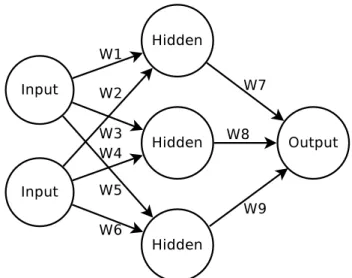
A simple application of EAs to the training of ANNs is the use of a standard GA to evolve the connection weights of a fixed topology network. Take an ANN of the form shown in Figure 2.6. Each of the connections in Figure 2.6 has an associated connection weight (wi). Assume also that each neuron uses a logistic sigmoid transfer function.
Here the NE method uses genotypes which comprise a string of floating point values describing the connection weights of each connection in the ANN. The genotypes are decoded into their corresponding phenotypes by assigning the connection weights to the predetermined topology; with the same connection weights always placed on the same connection. A genotype of this NE method, for this given topology, therefore takes the form of that given in Equation 2.14.
{w1, w2, w3, w4, w5, w6, w7, w8, w9} (2.14)
The fitness assigned to each genotype is then a measure of how well the decoded ANN performed on a given task. This fitness is then used to guide selection. Mutation is implemented by changing a given percentage of the connection weight values to a new random value. Crossover is implemented by creating child chromosomes which contain a proportion of the genes values from one parent, and the remainder from the other. The initial population is created by generating genotypes of random connection weight values. Finally, the search terminates when an ANN is found which performs suitably on the given task; or the maximum number of generations is reached.
As can be seen in this simple example, EAs can very easily be applied to the training of ANNs. However, even such a simple NE method has numerous advantages; as is discussed in Section 2.3. Additionally, many NE methods go beyond the simple application of a GA to the configuration of connection weights; as is described later in Section 2.6.
2.3
Advantages of NeuroEvolution
This section provides a number of possible advantages of using NE to train ANNs. These advantages are summarised as follows:
• Suited to supervised and reinforcement learning applications • Capable of training feed-forward and recurrent ANNs • Capable of training shallow and deep topologies • Capable of manipulating ANN topology
• No transfer function limitations
• Capable of creating homogeneous and heterogeneous ANNs • Always returns a solution
Of course there are also disadvantages of NE. For instance, like back propagation, NE is an iterative training process. This means that order of the training time is much larger than for non-iterative training methods such as RC [182]. Additionally, NE is a stochastic process which means the training time to produce its best solution varies, as does the quality of the final solutions found.
2.3.1 Application to Reinforcement Learning
In the field of machine learning there are three main types of learning; supervised, unsu-pervised and reinforcement. These are now briefly described.
The defining feature of supervised learning [163] is that it makes use of labelled data, that is, each training sample takes the form (xi, yi) where xi is an n-dimensional input
vector and yi is a discrete or continuous scalar associated with the input vector. The
system must learn to classify, or predict, the value ofyi based onxi. Supervised learning
systems are trained by showing sequences of training sets (xi, yi) in order for the system
can encode a relationshipf() between xi andyi;yi =f(xi).
Unsupervised learning [77], in contrast with supervised learning, uses unlabelled data
xi and attempts to find patterns and trends within that data. Unsupervised learning
systems are so called as they have no predefined measure of effectiveness and hence are unsupervised. Unsupervised learning is often used to cluster similar data sets or to predict future data sets based on previous examples.
Reinforcement learning [138] is where a system has to learn to perform a given task without any examples of desired behaviour, but where its behaviour can be given a per-formance value. The system has to take actions based on its current, and sometimes previous, inputs which are then given a score proportional to the desirability of the result of those actions. For example, if a human were to balance a broom upon their hand they have to learn in which direction to move their hand in order to keep the broom balanced. Bad actions in a given situation would see the broom fall from its central position and good movements would see the broom remain in, or approach, the central position. By noting which actions in which situations result in positive behaviour a human can learn to balance the broom. Reinforcement learning works much the same, there is no set of training examples to learn from, instead a system is given a score indicating its current performance i.e. the distance the broom is from vertical.
Generally the most popular training algorithms for ANNs allow ANNs to either be applied to supervised or unsupervised learning tasks. Common supervised learning meth-ods include back propagation [245] and radial basis function networks [180]. Common unsupervised learning methods include Hopfield networks [116] and restricted Boltzmann machines [260]. Additionally resent developments in deep belief neural networks, such as the application to playing GO [257], demonstrate a mechanism for training ANNs for reinforcement learning tasks. In such work the ANNs are trained using supervised learn-ing methods to predict the move chosen by expert GO players given a board state. This work effectively trained the ANNs as classifiers; a supervised learning task. The trained networks are then further trained using policy gradient reinforcement learning [270] to further the accuracy of the classifier. The trained networks are then used to estimate values of board states which is in turned used by Monte Carlo tree search [46].
As NE methods are based on EAs, they assess each solution by assigning a fitness value. This fitness value is representative of the ANN’s overall performance on a given task. Therefore, NE allows ANNs to be applied to reinforcement learning type tasks; tasks to which many standard ANN training methods cannot be applied. Additionally, as supervised learning tasks can be framed as reinforcement learning tasks, by looking at the overall performance rather than the performance on any particular sample, NE can also be used to train ANNs for supervised learning type tasks. As EAs cannot be applied to unsupervised learning this restriction also applies to NE.
to a wide range of applications; both supervised and reinforcement learning.
2.3.2 Recurrent Artificial Neural Networks
Another important benefit of NE is that it is not influenced by the topology of the ANN being trained. For instance, although back propagation can be extended to be capable of training RANN [19], by effectively “unwinding” the network, there are many unresolved issues [182]. One such issue is that as the error signal is propagated though the ANN it becomes weaker and the effect of training is diminished. This problem is increased if the error signal must traverse the network multiple times following the recurrent paths. Additionally, the computational expense of training increase proportionally to the depth of recurrence considered. Finally, as the error is only fed back a given number of times through the network, the result is always an approximation to the error at any given node, not the actual error.
As NE is not a function of the ANN topology these limitations simply do not apply. This is because NE training methods are not concerned with the internal state of the network at any given time, only the overall behaviour. Therefore, as long as a RANN can be applied to a problem and given some measure of fitness, it is no more complex, and has no more limitations, than training feed-forward ANNs.
2.3.3 Deep Artificial Neural Networks
Since the creation and demonstration of deep belief networks [108] by Geoffrey Hinton and Simon Osindero in 2006, the ability to train deep ANNs has been seen as increasingly significant. This is heightened by the fact that it is thought that deep ANNs can more efficiently implement a given function, in terms of the total number of nodes, than shallow networks [27].
However, back propagation alone has been shown to struggle to train deep ANNs [78, 178]; mainly due to the error gradient becoming smaller in magnitude as more layers are propagated. In resent work this issue has been overcome [79] via the use of rectifier neuron models.
Interestingly, as is described in the previous section, NE training algorithms are not a function of the ANN topology. NE can therefore be used to train deep ANNs without any alteration to the algorithm or use of rectifier neuron models.
2.3.4 Topology
It is known that the choice of topology has a large influence on the effectiveness of back propagation [178]. Additionally, there are no formal rules regarding the optimal/suitable choice of topology, only various “rules-of-thumb” [47]. A solution to this issue is to use training methods which adapt and find suitable topologies during training. To this end there are two common approaches used. 1) Constructive (growing) methods [168] start with a small number of hidden neurons (zero or one) and constructively add neurons during the search. 2) Destructive (pruning) [238] methods train using a large number of hidden neurons and destructively remove those which are unnecessary after the training is complete.
The constructive method of adding neurons is often considered suitable as it promotes the use of a minimal network sizes; aiding the generalisation of the ANN whilst keeping the dimensionality of the search low. When ANNs are trained on a data set for too long they begin to become capable of more accurately classifying samples within the training set at the expense of been able to correctly classify unseen samples. This phenomenon is referred to as over training. The ability to avoid this behaviour is referred to as generalisation. One method for avoiding over training is to limit the number of nodes available, ensuring that the ANN is not capable of very accurately classifying the training set, in order to preserve its ability to classify unseen items. For this reason constructive methods are often used as they are likely to create smaller, rather than larger, networks. It is also common to use regularization techniques with constructive method where the network is penalised for being too large; again favouring smaller networks. This method is often likened to the principle of Occam’s razor [30], where simpler solutions should be favoured over complex solutions if they are equivalent in quality.
Destructive methods (pruning) take the opposite approach. They train excessively large networks, which typically learn quickly and over train. Once trained, sections of the network which contribute the least to the output are removed. This method is thought to reduce the complexity of the network, reduce training time and aid generalisation. Destructive methods can be applied to any ANN regardless of how they have been trained and can therefore be used alongside other training methods, including NE [254], to aid generalisation.
However, destructive and constructive methods have their limitations. For instance iteratively adding neurons during the search is akin to topology hill climbing and is
sub-sequently likely to become trapped in topology local optima [15]. Destructive methods also have the issue of the user having to decide a suitably large number of neurons and requires careful removal of sections of the ANN post training.
In most cases however, the choice of topology is left to the user and a certain level of trial and error is often required in order to find suitable topologies. This is where many NE methods can offer a strong advantage. In the simplest case a standa