Civil Engineering Theses, Dissertations, and
Student Research Civil Engineering
Winter 11-3-2018
Effects of Moving Bottlenecks on Traffic
Operations on Four-lane Level Freeway Segments
Jianan ZhouUniversity of Nebraska - Lincoln, jianan.zhou@huskers.unl.edu
Follow this and additional works at:http://digitalcommons.unl.edu/civilengdiss
Part of theCivil Engineering Commons,Other Civil and Environmental Engineering Commons, and theTransportation Engineering Commons
This Article is brought to you for free and open access by the Civil Engineering at DigitalCommons@University of Nebraska - Lincoln. It has been accepted for inclusion in Civil Engineering Theses, Dissertations, and Student Research by an authorized administrator of
DigitalCommons@University of Nebraska - Lincoln.
Zhou, Jianan, "Effects of Moving Bottlenecks on Traffic Operations on Four-lane Level Freeway Segments" (2018).Civil Engineering Theses, Dissertations, and Student Research. 128.
EFFECTS OF MOVING BOTTLENECKS ON TRAFFIC OPERATIONS ON FOUR-LANE LEVEL FREEWAY SEGMENTS
by
Jianan Zhou
A DISSERTATION
Presented to the Faculty of
The Graduate College at the University of Nebraska In Partial Fulfillment of Requirements For the Degree of Doctor of Philosophy
Major: Civil Engineering
(Transportation Systems Engineering)
Under the Supervision of Professors Laurence R. Rilett and Elizabeth G. Jones
Lincoln, Nebraska
EFFECTS OF MOVING BOTTLENECKS ON TRAFFIC OPERATIONS ON FOUR-LANE LEVEL FREEWAY SEGMENTS
Jianan Zhou, Ph.D. University of Nebraska, 2018 Advisor: Laurence R. Rilett (Chair), Elizabeth G. Jones (Co-chair)
The Highway Capacity Manual (HCM) was developed to provide capacity and level of service analyses for roadway facilities. Trucks may adversely affect the quality of traffic flow on a roadway. In HCM, the passenger car equivalent (PCE) of a truck, which represents the number of passenger cars that have an equivalent effect on traffic flow, is used to account for the impacts of trucks.
However, in the past ten years rural freeways in the western rural U.S. have experienced conditions that lie outside the standard HCM conditions. Also, the current HCM truck PCEs may not be appropriate for the western rural U.S. This is because, the interstates in the western rural U.S. consistently experience truck percentages in an excess of 25 percent, but the highest truck percentage published in current HCM is 25 percent. Additionally, there are large free-flow speed differences between heavy trucks and passenger cars in western rural U.S., however, the current HCM estimates the PCEs under the assumption that trucks maintain the same speed as passenger cars on level terrain. Compounding the above two issues, trucks passing other trucks at low speed differentials may cause moving bottlenecks.
This dissertation proposed a definition, developed identification methods for the moving bottlenecks on four-lane freeway segments, and developed metrics for measuring their effects. Then, this dissertation calculated PCEs under western rural U.S. traffic flow
conditions with localized congestion caused by moving bottlenecks, by equal-density and equal-capacity method. Finally, this dissertation explored the impacts of changes in speed limits, truck passing restriction and data aggregation interval on PCEs.
The results demonstrate moving bottlenecks have an adverse effect on vehicles on the freeway. It was found that the PCE values in the HCM 2010 and HCM 2016
underestimate the effect of heavy trucks on level terrain freeways that experience high truck percentage, and where different vehicle types have large differences in average free-flow speeds. The results also show that speed limits, percentage of truck passing restriction, and data aggregation interval significantly affect the PCEs. The results will be helpful in understanding how trucks affect passenger cars in moving bottlenecks.
DEDICATION
ACKNOWLEDGMENTS
I would like to first sincerely thank my committee chair, Dr. Laurence Rilett for his professional guidance, inspiration and financial support during my Ph.D. studies at University of Nebraska-Lincoln. He always passes his enthusiasm about the research to me, and always leads to me to think positively and creatively. I would also like to sincerely thank my committee co-chair, Dr. Elizabeth Jones for her expertise and encouragement during my Ph.D. studies. I will always remember her willingness to see my success in academic and personal development.
I would also like to thank Dr. Aemal Khattak and Dr. Kathryn Hanford for serving on my committee and for sharing their knowledge and experience with me.
I would like to thank the Nebraska Department of Transportation, Mid-America Transportation Center and the Nebraska Transportation Center for providing the
resources and facilities to complete this research. I would also like to express my deep appreciation to Dr. George List and his colleagues at North Carolina State University for their information provided related to the 2016 HCM PCE estimation methodology.
My sincere thanks also go to Yifeng (Chaser), Li, Ernest, Huiyuan, Yashu, Amirfarrokh, Myungwoo, Waleed, Huong, Larissa, Amber, Huiling, and all my fellow students and all the staff and all the visiting scholars at NTC who have helped me with my research and also my everyday life.
Finally, I would like to thank my dear Mom and Dad and my families, and all my friends in China and in U.S. who have accompanied me on this long journey. Special thanks to my dear wife, for waiting for me four years. It is your love and courage that makes me confident to get a degree. I cherish you so much.
TABLE OF CONTENTS
CHAPTER 1 INTRODUCTION ... 1
1.1 Problems Introduction ... 1
1.2 Research Objective and Tasks ... 2
1.3 Definition of “Western Rural U.S.” Freeway Segments... 3
CHAPTER 2 BACKGROUND, LITERATURE REVIEW AND ISSUE STATEMENTS... 8
2.1 Trucks Definitions and Characteristics ... 8
2.2 Characteristics of Traffic Flow on Interstate 80 in Nebraska ... 9
2.3 Research on Moving Bottlenecks Identification ... 9
2.4 Research on Metrics for Level-of-Service of Uninterrupted Traffic Flow .. 10
2.5 Research on Passenger Car Equivalents ... 12
2.5.1 Overview ... 12 2.5.2 Equal-Density (HCM 2010) Method ... 15 2.5.3 Equal-Capacity (HCM 2016) Method ... 17 2.5.4 Equal-Impedance Method ... 19 2.5.5 Overtaking Method ... 22 2.5.6 Headway-Based Method ... 23 2.5.7 Delay-Based Method ... 24 2.5.8 Speed-Area-Based Method ... 25 2.5.9 Travel-Time-Based Method ... 26 2.5.10 Platoon-Based Method ... 27 2.5.11 Speed-Based Method ... 28 2.5.12 Equal-Flow Method ... 29
2.5.13 Queue Discharge Flow Method ... 30
2.6 Research on Development and Calibration of Microscopic Traffic Simulation Models ... 31
2.7 Research on Influencing Factor Analysis for Passenger Car Equivalents ... 33
2.8.1 Issues in PCE at Level Freeway Segments in HCM 2010 and HCM
2016 ... 35
2.8.2 Issues in Other PCE Methodologies ... 37
2.8.3 Issues in Moving Bottlenecks Identification ... 38
2.8.4 Issues in Metrics for Moving Bottlenecks Effects ... 39
2.8.5 Other Issues ... 40
CHAPTER 3 HYPOTHESIS STATEMENT ... 41
CHAPTER 4 DATA COLLECTION AND PRELIMINARY ANALYSIS ... 44
4.1 Data Collection Sites... 44
4.2 Data Collection Methodology ... 47
4.2.1 Equipment ... 47
4.2.2 Sensor Calibration ... 49
4.3 Data Collection ... 50
4.4 Preliminary Analysis ... 53
4.4.1 Vehicle Classification ... 53
4.4.2 Vehicle Composition Analysis ... 53
4.4.3 Speed Distribution ... 60
4.5 Summary ... 62
CHAPTER 5 HIGHWAY CAPACITY ANALYSIS BY HCM 2010 AND 2016 APPROACH ... 63
5.1 Recommended PCE Values in HCM 2010 and 2016 ... 63
5.1.1 Recommended PCE Values in HCM 2010 ... 63
5.1.2 Recommended PCE Values in HCM 2010 ... 66
5.2 Operational Analysis ... 73
5.2.1 Operational Analysis with Empirical Data ... 73
5.2.2 Comparison Between Empirical Data and HCM 2010/2016 Operational Analysis Results ... 81
5.3 Summary ... 86
CHAPTER 6 MOVING BOTTLENECKS AND LOCALIZED CONGESTION ANALYSIS ... 88
6.1 Moving Bottlenecks Identification ... 88
6.1.1 Moving Bottlenecks Definition... 88
6.1.2 Critical Headway and Free Vehicles Identification ... 91
6.1.3 Frequency and Percentage of In-moving-Bottlenecks and Free Vehicles ... 92
6.1.4 Moving Bottlenecks Type and Vehicle Type ... 94
6.2 Analysis for Impeded and Free-flow Vehicles ... 98
6.2.1 Definition of Impeded and Free Vehicles ... 98
6.2.2 Frequency and Percentage of Impeder, Impeded, and Free Vehicles ... 99
6.2.3 Speed Distribution for Impeded and Free Vehicles ... 102
6.2.4 Additional Analysis for Impeded and Free Vehicles ... 103
6.3 Moving Bottlenecks Characteristics ... 107
6.3.1 Overview of Moving Bottlenecks Characteristics ... 107
6.3.2 Speed-related Moving Bottleneck Characteristics ... 107
6.3.3 Spatial-related Moving Bottlenecks Characteristics ... 117
6.3.4 Characteristics related to Moving Bottlenecks Existence ... 119
6.4 Metrics for Localized Congestion ... 125
6.5 Summary ... 133
CHAPTER 7 CALCULATING PCES BASED ON EQUAL-DENSITY METHOD . ... 135
7.1 Simulation Model Development for Equal-Density Method ... 135
7.1.1 Description of Simulation Model... 135
7.1.2 Simulation Model Calibration... 144
7.1.3 Simulation Approach ... 152
7.2 PCE Based on Equal-density Method ... 154
7.2.1 ED_PCE Estimation Results ... 154
7.2.2 Influencing Factor Analysis ... 157
7.3 Comparison between ED_PCEs and the Recommended PCEs in HCM 2010 ... 159
7.4 Summary ... 163
CHAPTER 8 CALCULATING PCES BASED ON EQUAL-CAPACITY METHOD ... 165
8.1 Simulation Model Development for Equal-Capacity Method ... 165
8.2 Procedure for PCE Estimation Based on Equal-capacity Method ... 173
8.3 PCE Based on Equal-Capacity Method ... 187
8.3.1 EC_PCE Estimation Results ... 187
8.3.2 Influencing Factor Analysis ... 202
8.4 Comparison between EC_PCEs and the Recommended PCEs in HCM 2016 ... 203
8.5 Applicable Conditions for EC_PCEs and the Recommended PCEs in HCM 2016 ... 206
8.6 Summary ... 216
CHAPTER 9 SENSITIVITY ANALYSIS FOR WESTERN RURAL U.S. EC_PCES ... 218
9.1 Sensitivity Analysis for EC_PCEs Based on Speed Limit Changes ... 218
9.1.1 Overview of Speed Limit ... 218
9.1.2 EC_PCEs at Different Speed Limit Level ... 224
9.1.3 Impacts of Speed Limits on EC_PCEs ... 230
9.2 Sensitivity Analysis for EC_PCEs Based on Truck Passing Restriction ... 232
9.2.1 Overview of Truck Passing Restriction ... 232
9.2.2 EC_PCEs at Different Truck Passing Restriction Levels ... 234
9.2.3 Impacts of Truck Passing Restriction on PCEs ... 240
9.3 Sensitivity Analysis for EC_PCEs Based on Data Aggregation Interval .. 243
9.3.1 Overview of Data Aggregation Interval ... 243
9.3.2 EC_PCEs at Different Data Aggregation Interval ... 244
9.3.3 Impacts of Data Aggregation Interval on EC_PCEs... 250
9.4 Summary ... 252
CHAPTER 10 CONCLUDING REMARKS... 254
10.2 Contributions... 258 10.3 Recommendations for Future Research ... 259 REFERENCES ... 261 APPENDIX A DETAILS OF WESTERN RURAL U.S. FREEWAY SEGMENTS .... 273 APPENDIX B DATA COLLECTION SITES ... 275 APPENDIX C RELATIONSHIP BETWEEN AVERAGE SPEED AND HEADWAY FOR DIFFERENT HEADWAY TYPE... 281 APPENDIX D THEORETICAL ANALYSIS FOR MOVING BOTTLENECK
EXISTENCE TIME AND DISTANCE ON TWO LANES WITH DIFFERENT
MOVING BOTTLENECK SPEED DIFFERENCE ... 285 APPENDIX E RESULTS OF THEORETICAL ANALYSIS FOR EFFECTS OF
PLATOON SPEED DIFFERENCE ... 287 APPENDIX F VOLUME-DENSITY CURVES IN ED_PCES ESTIMATION ... 289 APPENDIX G EXAMPLES OF SCATTER PLOTS IN EC_PCE ESTIMATION... 297 APPENDIX H EC_PCE AS FUNCTION OF SPEED LIMIT LEVEL FOR ALL
LENGTH... 303 APPENDIX I EC_PCE AS FUNCTION OF TRUCK RESTRITION LEVEL FOR ALL LENGTH... 307 APPENDIX J EC_PCE AS FUNCTION OF DATA AGGREGATION INTERVAL LEVEL FOR ALL LENGTH ... 312
LIST OF FIGURES
Figure 1.1 Interstate with two lanes per direction and speed limit of 75 mph or
higher in western U.S. ... 4
Figure 1.2 Interstate with truck percentage higher than 25 percent in western U.S. .. 5
Figure 1.3 Western Rural U.S. freeway segments based on criteria in Table 1-1 ... 6
Figure 2.1 FHWA 13-category vehicle classifications ... 8
Figure 2.2 Volume-density curves for estimating PCEs using equal-density method ... 16
Figure 2.3 Impedance-flow relationships for equal impedance method ... 21
Figure 4.1 I-80 Data collection sites between Lincoln and North Platte ... 45
Figure 4.2 NTC’s ITS data collection van ... 47
Figure 4.3 Layout of virtual speed detectors on video ... 48
Figure 4.4 Hourly volumes for each classification ... 58
Figure 4.5 Percentages of vehicles for each classification ... 59
Figure 4.6 Speed distribution for all vehicles ... 61
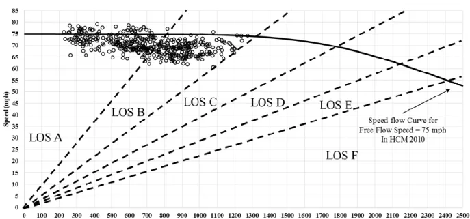
Figure 5.1 The observed traffic flow, FFS = 75 mph speed-flow curve, and the operational analysis results with PCE = 1.5 in HCM 2010 ... 82
Figure 5.2 Operational analysis results (LOS) using PCE = 1.5 in HCM 2010 ... 83
Figure 5.3 The observed traffic flow, FFS = 75 mph speed-flow curve, and the operational analysis results with PCE for level freeway segments in HCM 2016 ... 84
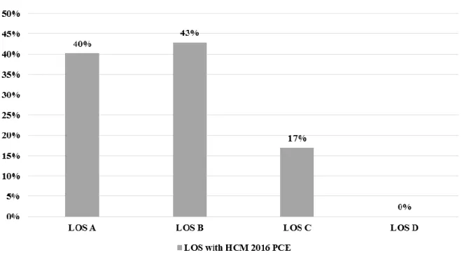
Figure 5.4 Operational analysis results (LOS) using PCE for level freeway segments in HCM 2016 ... 85
Figure 6.1 Moving-bottlenecks definition ... 89
Figure 6.2 Frequency of vehicles in moving bottlenecks ... 93
Figure 6.3 Frequency of vehicles in moving bottlenecks ... 93
Figure 6.4 Frequency of moving bottleneck types ... 94
Figure 6.5 Percentage of moving bottleneck types ... 95
Figure 6.6 Frequency of vehicle type ... 97
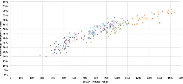
Figure 6.8 Frequency of impeder, impeded and non-impeded vehicles ... 99 Figure 6.9 Percentage of impeder, impeded and non-impeded vehicles ... 100 Figure 6.10 Speed distribution for impeded and non-impeded vehicles ... 101 Figure 6.11 Relationship between traffic volume and amount of impeded vehicle 104 Figure 6.12 Relationship between traffic volume and percentage of impeded vehicle
... 105 Figure 6.13 Relationship between traffic volume and percentage of time impeding
... 106 Figure 6.14 Impeded vehicle speed vs non-impeded vehicle speed (for all vehicles)
... 108 Figure 6.15 Impeded vehicle speed vs non-impeded vehicle speed (for passenger
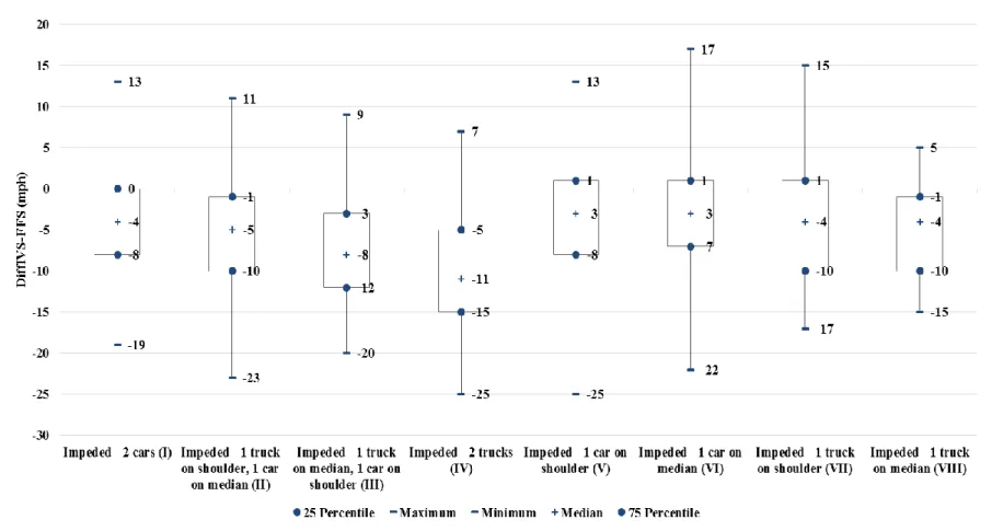
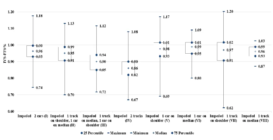
cars) ... 109 Figure 6.16 Impeded vehicle speed vs non-impeded vehicle speed (for trucks) .... 110 Figure 6.17 Distribution of DiffIVS-FFS for each moving bottleneck type ... 114 Figure 6.18 Distribution of IVS-FFS% for each moving bottleneck type ... 116 Figure 6.19 Average number of impeded vehicles for different moving-bottleneck
types ... 118 Figure 6.20 Average density of impeded vehicles for different moving-bottleneck
types ... 118 Figure 6.21 Definition of moving bottleneck existence distance and existence time
... 120 Figure 6.22 Moving-bottleneck existence distance and time for different
moving-bottleneck types based on empirical data ... 124 Figure 6.23 Moving-bottleneck delay for passenger cars with FFS = 75 mph based
on empirical data ... 124 Figure 6.24 Variables for localized congestion analysis ... 128 Figure 6.25 Explanation of the meaning of DUF - an example of high DUF value
... 131 Figure 6.26 Explanation of the meaning of DUF - an example of low DUF value 132 Figure 6.27 Definition of density uniformity factor (DUF) ... 133
Figure 7.1 Simulation model developed in CORSIM 6.3 for equal-density method
Figure 7.2 Simulation model developed in VISSIM 9.0 for equal-density method 141 Figure 7.3 Single free-flow speed distributions for all vehicle types in VISSIM 9.0
for equal-density method ... 143
Figure 7.4 Empirical free-flow speed distributions for different vehicle types in VISSIM 9.0 for equal-density method ... 143
Figure 7.5 The best MAER at each generation for equal-density method ... 151
Figure 7.6 The best fitness at each generation for equal-density method ... 151
Figure 7.7 ED_PCEs with a single free-flow speed in CORSIM 6.3 ... 155
Figure 7.8 ED_PCEs with a single free-flow speed distribution in VISSIM 9.0 ... 156
Figure 7.9 ED_PCEs with empirical free-flow speed distributions in VISSIM 9.0 157 Figure 7.10 Relationship between observed traffic flow and FFS = 75 mph speed-flow curve in HCM 2010 with PCE = 1.5 ... 161
Figure 7.11 Relationship between observed traffic flow and FFS = 75 mph speed-flow curve in HCM 2010 with new ED_PCEs ... 162
Figure 7.12 Comparison of LOS results between using PCE = 1.5 and new ED_PCEs ... 163
Figure 8.1 Free-flow speed distributions for free vehicles on level terrain under HCM 2016 and western rural U.S. (Nebraska empirical) conditions ... 166
Figure 8.2 Truck length distributions under HCM 2016 and western rural U.S. (Nebraska empirical) conditions ... 167
Figure 8.3 Weight distributions for SUTs and TTs for equal-capacity method ... 169
Figure 8.4 Horsepower distributions for SUTs and TTs for equal-capacity method ... 170
Figure 8.5 Schematic of the simulation model for equal-capacity PCE estimation 171 Figure 8.6 The best MAER at each generation for equal-capacity method ... 172
Figure 8.7 The best fitness at each generation for equal-capacity method ... 173
Figure 8.8 Flow-density scatter plots for the auto-only flow at 1% grade, 1.5 miles distance under HCM 2016 conditions ... 188
Figure 8.9 Flow-density scatter plots for the mixed flow at 10% truck percentage, 30% SUT/70% TT truck composition, 1% grade, 1.5 miles distance under HCM 2016 conditions ... 189
Figure 8.10 Simulated and estimated CAF for 30% SUT/70% TT truck compositions ... 191
Figure 8.11 Simulated and estimated CAF for 50% SUT/50% TT truck compositions
... 191
Figure 8.12 Simulated and estimated CAF for 70% SUT/30% TT truck
compositions ... 192 Figure 8.13 Equal-capacity-based PCE estimation results for 30% SUT, 70% TT,
0% grade ... 200 Figure 8.14 Equal-capacity-based PCE estimation results for 50% SUT, 50% TT,
0% grade ... 200 Figure 8.15 Equal-capacity-based PCE estimation results for 70% SUT, 30% TT,
0% grade ... 201 Figure 8.16 The observed traffic flow, FFS = 75 mph speed-flow curve in HCM
2016, and the operational analysis results with PCE for level freeway segment in HCM 2016 ... 204 Figure 8.17 The observed traffic flow, FFS = 75 mph speed-flow curve in HCM
2016, and the operational analysis results with proposed EC_PCEs (western rural U.S. conditions) ... 205
Figure 8.18 Comparison of LOS results between using recommended PCEs in HCM
2016 and proposed EC_PCEs (one-minute interval, western rural U.S.
condition) ... 205 Figure 8.19 Simulation model for capturing localized congestion ... 207 Figure 8.20 Heat map for the density at time period 𝑖 at freeway segment 𝑗 under
HCM 2016 conditions ... 209 Figure 8.21 Heat map and for the density at time period 𝑖 at freeway segment 𝑗
under western rural U.S. conditions ... 210 Figure 8.22 Density uniformity factor over 60 consecutive time periods at freeway
segments 𝑗 (𝐷𝑈𝐹𝑗) under HCM 2016 and western rural U.S. conditions ... 211 Figure 8.23 Density uniformity factor over 24 consecutive freeway segments at time
period 𝑖 under HCM 2016 and western rural U.S. conditions (𝐷𝑈𝐹𝑖) ... 211
Figure 8.24 The relationship between EC_PCEs and DUFs for each simulation
scenario ... 215 Figure 9.1 Free-flow speed distributions for different vehicle types at speed limit 70
Figure 9.2 Free-flow speed distributions for different vehicle types at speed limit 75 mph ... 223 Figure 9.3 Free-flow speed distributions for different vehicle types at speed limit 80
mph ... 223 Figure 9.4 Free-flow speed distributions for different vehicle types at speed limit 85
mph ... 224 Figure 9.5 Comparison of EC_PCEs among different speed limits at (a) 30%
SUT/70% TT (b) 50% SUT/50% TT and (c) 70% SUT/30% TT with no truck passing restriction, 1-minute data aggregated interval, 0% grade, and 1.5 miles grade length ... 230 Figure 9.6 Comparison of EC_PCEs among different percentages of truck passing
restriction at (a) 30% SUT/70% TT (b) 50% SUT/50% TT and (c) 70% SUT/30% TT with 75 mph speed limit, 1-minute data aggregated interval, 0% grade, and 1.5 miles grade length. ... 240 Figure 9.7 Comparison of EC_PCEs among different data aggregation interval at (a)
30% SUT/70% TT (b) 50% SUT/50% TT and (c) 70% SUT/30% TT with 75 mph speed limit, no truck passing restriction, 0% grade, and 1.5 miles grade length ... 250
LIST OF TABLES
Table 1.1 Criteria for western rural U.S. freeway segments ... 3 Table 2.1 Critical headway values in previous research ... 10 Table 2.2 Explanation of metrics for level-of-service of uninterrupted traffic flow 12 Table 2.3 Summary of places that PCE methodologies used ... 14 Table 4.1 Data collection sites along I-80 on western part of Nebraska, between
Lincoln and North Platte ... 46 Table 4.2 Summary of data collection ... 52 Table 4-3 Total number of vehicles for each classification ... 54 Table 4.4 Hourly volumes for each vehicle classification on all data collection sites
(veh/h) ... 56 Table 4.5 Percentages of vehicles for each classification ... 57 Table 5.1 PCE value in HCM 2010 for freeway by type of terrain ... 63 Table 5.2 PCE value in HCM 2010 for freeway at level terrain by proportion of
trucks ... 64 Table 5.3 PCE value in HCM 2016 for freeway by type of terrain ... 66 Table 5.4 PCE value in HCM 2016 for freeway at level terrain by proportion of
trucks with 70% heavy trucks, 30% single-unit trucks ... 67 Table 5.5 PCE value in HCM 2016 for freeway at level terrain by proportion of
trucks with 50% heavy trucks, 50% single-unit trucks ... 69 Table 5.6 PCE value in HCM 2016 for freeway at level terrain by proportion of
trucks with 30% heavy trucks, 70% single-unit trucks ... 71 Table 5.7 LOS criteria for basic freeway segment (HCM 2010 and HCM 2016) .... 77 Table 6.1 Results of critical headway determination ... 92 Table 6.2 Summary of moving bottleneck type ... 94 Table 6.3 Summary of vehicle type ... 96 Table 6.4 Results of T-test for comparisons between impeded and non-impeded
vehicle speed... 102 Table 6.5 Results of T-test for comparisons for speed of impeded vehicles ... 112
Table 6.6 Theoretical analysis for effects of moving bottleneck speed difference on moving bottleneck existence time, distance and moving bottleneck delay for passenger cars with FFS = 75 mph ... 123 Table 6.7 Empirical analysis for average moving bottleneck existence time, distance
and moving bottleneck delay for passenger cars with FFS = 75 mph ... 123 Table 7.1 Geometric, vehicles, and traffic characteristics for CORSIM 6.3
simulation model ... 137 Table 7.2 Geometric, vehicles, and traffic characteristics for VISSIM 9.0 simulation
model ... 138 Table 7.3 Average ED_PCEs with a single free-flow speed in CORSIM 6.3 ... 154 Table 7.4 Average ED_PCEs with a single free-flow speed distribution in VISSIM
9.0 ... 156 Table 7.5 Average ED_PCEs with empirical free-flow speed distributions in
VISSIM 9.0 ... 157 Table 7.6 Results of ANOVA analysis for ED_PCEs ... 159
Table 7.7 Comparison between the new ED_PCEs with the recommended PCEs in
HCM 2010 ... 160 Table 8.1 Key parameters for HCM 2016 and western rural U.S. conditions in
VISSIM 9.0 simulation model ... 168 Table 8.2 Parameters in the models for CAF estimation ... 193 Table 8.3 Estimated CAFs for different truck percentage and distance at 0% grade at
30% SUT, 70% TT ... 194 Table 8.4 Estimated CAFs for different truck percentage and distance at 0% grade at
50% SUT, 50% TT ... 195 Table 8.5 Estimated CAFs for different truck percentage and distance at 0% grade at
70% SUT, 30% TT ... 196 Table 8.6 Equal-capacity-based PCE estimation results at level freeway segments
(0% Grade) with 30% SUT, 70% TT ... 197 Table 8.7 Equal-capacity-based PCE estimation results at level freeway segments
(0% Grade) with 50% SUT, 50% TT ... 198 Table 8.8 Equal-capacity-based PCE estimation results at level freeway segments
(0% Grade) with 70% SUT, 30% TT ... 199 Table 9.1 Speed limit of rural freeway segments for each state in U.S. ... 220
Table 9.2 Parameters in the models for CAF estimation at 70 mph and 75 mph speed limit ... 225 Table 9.3 Parameters in the models for CAF estimation at 80 mph and 85 mph speed limit ... 226 Table 9.4 EC_PCE results as a function of speed limit level (0% grade and 1.5 mile
grade length) ... 228 Table 9.5 Results of ANOVA and comparison test for EC_PCEs related to speed
limit ... 231 Table 9.6 Parameters in the models for CAF estimation at 0%, 25% and 50% truck
passing restriction ... 235 Table 9.7 Parameters in the models for CAF estimation at 50% and 75% truck
passing restriction ... 236 Table 9.8 EC_PCE results as a function of truck passing restriction level (0% grade
and 1.5 mile grade length) ... 238 Table 9.9 Results of ANOVA and comparison tests for EC_PCEs related to truck
passing restriction ... 241 Table 9.10 Parameters in the models for CAF estimation at 1, 5 and 10 minutes
intervals ... 245 Table 9.11 Parameters in the models for CAF estimation at 15 and 20 minutes
intervals ... 246 Table 9.12 EC_PCE results as a function of data aggregation interval level (0%
grade and 1.5 mile grade length) ... 248 Table 9.13 Results of ANOVA and comparison tests for EC_PCEs related to data
CHAPTER 1 INTRODUCTION
1.1 Problems Introduction
Trucks may adversely affect the quality of traffic flow on a roadway due to the fact that
1)The average space occupied by a truck is greater than that of a passenger car; 2)The vehicle performance (e.g. acceleration, deceleration, maneuverability,
operating speed, etc.) of trucks are typically lower than that of passenger cars. In the Highway Capacity Manual (HCM), the passenger car equivalent (PCE) of a truck, which represents the number of passenger cars that would have an equivalent effect on the traffic flow as a given truck type (1), is used to account for the presence of trucks in a traffic flow. PCEs allow a heterogeneous mix of vehicles in a traffic stream to be expressed as a standardized, homogenous traffic stream of passenger cars.
However, the HCM truck PCE values may not be appropriate for the western rural U.S. This is because
1) The interstates in western rural U.S. consistently experience truck percentages in an excess of 25 percent, but the highest truck percentage value published in either HCM 2010 or HCM 2016 is 25 percent;
2) There are large free-flow speed differences between heavy trucks and passenger
cars in western rural U.S., however, the HCM 2010 and HCM 2016 estimate the PCEs under the assumption that trucks maintain the same speed as passenger cars on level terrain (2)(3);
3) Compounding the above two issues, trucks passing other trucks at low speed differentials (e.g., a 67 mph truck passing a 66 mph truck) may cause moving bottlenecks.
Thus, this dissertation aims at estimating new PCEs under the western rural U.S. traffic conditions with localized congestion caused by moving bottlenecks.
1.2 Research Objective and Tasks
Because of the problems above, the main objectives in this dissertation include 1) Proposing a definition, developing identification methods for the moving
bottlenecks on four-lane freeway segments, and developing metrics for measuring their effects;
2) Calculating PCEs under western rural U.S. traffic flow conditions with localized congestion caused by the moving bottlenecks. The results should be compared and evaluated with the values in corresponding original research;
3) Exploring the impacts of changes in speed limits, truck passing restriction and data aggregation interval on PCEs.
To achieve the research objectives above, there are eight tasks in this dissertation: Task 1: Perform a literature review and analyze current issues (Chapter 2);
Task 2: Propose hypotheses (Chapter 3);
Task 3: Define study area, collect field data, and preliminary analysis (Chapter 4); Task 4: HCM-standard operating analysis with empirical data (Chapter 5);
Task 5: Moving bottlenecks analysis with empirical data (Chapter 6); Task 6: Developing simulation model (Chapter 7 and Chapter 8);
Task 7: Calculating PCEs based on existing methods under western rural U.S. conditions and making comparison with the original research (Chapter 7 and Chapter 8);
Task 8: Exploring the impacts of speed limits, truck passing restriction and data aggregation interval on PCEs (Chapter 9).
The results will be helpful in understanding how trucks affect passenger cars and how moving bottlenecks affect traffic flow on four-lane level freeway segments.
1.3 Definition of “Western Rural U.S.” Freeway Segments
This research focuses on freeway segments in the western rural U.S. The term “western rural U.S.” freeway segment is defined according to the four criteria outlined in Table 1.1.
Table 1.1 Criteria for western rural U.S. freeway segments
No. Criteria
1 Passenger car and/or truck speed limit equal to or higher than 75 mph.
2 Desired free flow speeds for commercial trucks (e.g. FHWA classification 5 to
13) (4) that are lower (e.g. 5 mph) than the passenger car speed limit.
3 Truck percentages higher than 25 percent.
4 U.S. interstate, or highways designed to U.S. interstate standards (5), with two lanes per direction (divided).
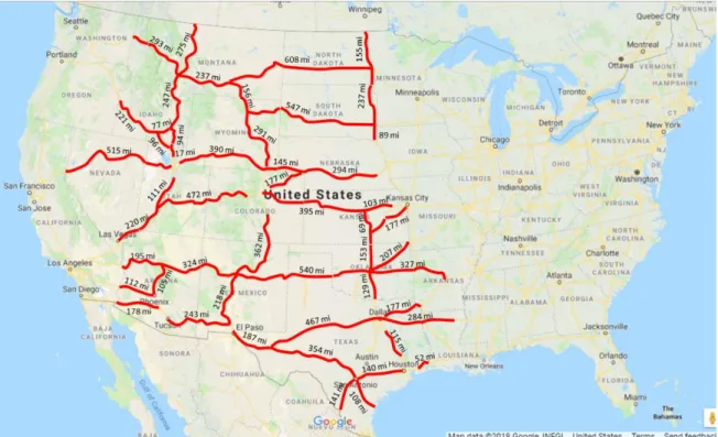
1) Note that interstate style roadways with two lanes in each direction (e.g. criteria 4) and with speed limits of 75 mph or higher (e.g. criteria 1) are mainly found in the western U.S. (6) as shown in Figure 1.1 (6-28).
Figure 1.1 Interstate with two lanes per direction and speed limit of 75 mph or higher in western U.S.
2) Criteria 2 may occur as a result of a) speed limiters implemented by the truck owners, and/or b) speed limit for trucks lower than the speed limit for passenger cars.
3) Truck percentages higher than 25 percent (e.g. criteria 3) are relatively rare in areas of the U.S. where the population density is relatively high. However, in many locations in the western U.S., particularly where population density is low,
the high truck percentages can be relatively high. The highways shown in red in Figure 1.2 indicate the locations on the interstate system where truck percentages may exceed 25 percent on a regular basis (7-28). High truck percentages rarely, if ever, occur in urban areas. Regardless, freeway segments that experience low passenger car volumes and relatively high truck volumes, where the trucks travel as considerably lower speeds, are susceptible to the creation of moving
bottlenecks as will be discussed in detail in Chapter 6.
Figure 1.2Interstate with truck percentage higher than 25 percent in western U.S.
Based on the criteria in Table 1.1 the “western rural U.S. freeway” segments that are the focus of this dissertation are shown in red in Figure 1.3. Complete details regarding these segments may be found in the appendix. Note that this figure is based on available
information (7-28) and may not be comprehensive. Freeways that met the four criteria listed in Table 1.1 comprise 11,826 miles of the U.S. Interstate Highway System.
Figure 1.3 Western Rural U.S. freeway segments based on criteria in Table 1.1
It should be noted this research is based on the traffic flow data collected from I-80 between Lincoln and North Platte in Nebraska, which is a typical example of the “western rural U.S.” freeway segment. It is hypothesized that the methodologies and concluding remarks in this research may be generalized to the other “western rural U.S.” freeway segments shown in Figure 1.3. Note that this is no different than the hypothesis implicit in the HCM where the PCE values that were developed for three lane freeways and modeled using a traffic simulation model calibrated to conditions found on the east coast of the U.S. are assumed to apply across the U.S. The hypothesis in this dissertation is that the PCE values developed in this research will be better estimates of the PCE values on the western
rural U.S. freeways than the 2016 HCM values. If there are any doubts about which PCE values to use the methodology used in this dissertation may be readily used by traffic agencies to develop PCE values for their local conditions.
Lastly, the methodology discussed in this dissertation was developed from empirical data obtained from level terrain as defined in the 2016 HCM (3). For rolling and
mountainous terrain the methodology can be replicated relatively easily. Note that Figure 1.3 does not differentiate among level, rolling and mountainous terrain.
CHAPTER 2 BACKGROUND, LITERATURE REVIEW AND ISSUE STATEMENTS
2.1 Trucks Definitions and Characteristics
The FHWA 13-Category Rule Set standardized vehicle classification system, developed by FHWA in the mid-1980s, currently serves as the basis for state vehicle classification counting efforts (4). The FHWA classification is shown in Figure 2.1. Vehicles are classified into the following 6 groups: motorcycles (class 1); passenger cars, pickups, vans, and vehicles with trailers (classes 2 and 3); buses (class 4); single-unit trucks (classes 5, 6, and 7); recreational vehicles (class 5); and heavy trucks (classes 8 to 13).
2.2 Characteristics of Traffic Flow on Interstate 80 in Nebraska
In Nebraska, Interstate 80 (I-80) is 456 miles in length. This research focuses on the section between the milepost 177 near to North Platte and the milepost 399 near to Lincoln. According to Statewide Traffic Flow Map for Nebraska in 2014 (7), this section the AADT (average annual day traffic volume) is between 15,265 veh/d and 25,930 veh/d. The AADT for trucks is between 6,960 veh/d and 8,490 veh/d. The truck percentage based on AADT ranges between 31% and 49%. The Statewide Traffic Flow Map for Nebraska in 2014 shows that
1) The traffic volume decreases from east to west, and the decrease rate of passenger car volumes are higher than truck volumes;
2) The truck percentage increases while the passenger car percentage decreases from east to west, and the truck percentage is higher than 25% for the entire section;
3) The higher truck percentage usually appears with lower traffic volume and vice versa.
2.3 Research on Moving Bottlenecks Identification
Moving bottlenecks are defined as the queuing caused by a slow-moving vehicle during periods of moderate to heavy demand (29). Such queuing can occur not only on a single lane of traffic, but also on multilane highways, even though only one of the lanes appears to be obstructed by the slow moving vehicle. In general, a moving bottleneck is caused by the fast vehicles catching up with the slower vehicles and not being able to pass. Vehicles that do not catch up with other vehicles or are not impeded by other vehicles are
defined as “free vehicles.” One accepted definition of a free vehicle is that its speed is not influenced by the speed of the vehicle traveling ahead of it (30 and 31). In this research, a moving bottleneck is defined as a group of vehicles traveling on either the median or the shoulder lane in the same direction, where one influences the speed of the other.
The identification for moving bottlenecks on two-lane highway, referred to as platoons, has been widely researched. Platoons are usually identified by headways between the leading and following vehicles. In order to be considered as a vehicle in platoons, the headways should not be greater than a specific threshold (32 and 33). The threshold for platoon identification is defined as the “critical headway”. The values of critical headway vary among researchers. A detailed explanation of critical headway may be found in Table 2.1. The previous research shows that the critical headway varies among different road type and traffic conditions.
Table 2.1 Critical headway values in previous research
Literature Critical Headway Value
HCM 2010 and HCM 2016(2)(3) 3s (two-lane highway)
Miller 1961(87) 8s (two-lane highway)
Edie et al 1963(88) 4s to 5s (two-lane highway)
Keller 1976(89) 2s (two-lane highway)
Al-Kaisy and Karjala 2010(31) 6s (two-lane rural highway)
Fitzpatrick et al 2004(90) 5s for leading headway, 3s for lagging headway (two-lane highway)
2.4 Research on Metrics for Level-of-Service of Uninterrupted Traffic Flow
In HCM 2010 and HCM 2016, for freeway and multilane highway segments, the density is used as the measure of effectiveness for level-of-service (LOS). For two-lane
highway segments, the LOS measures of effectiveness include average travel speed (ATS), percent time spent following (PTSF), and percentage of free-flow speed (PFFS). In previous research other popular LOS metrics include the average travel speed of passenger cars (ATSPC), the percentage of free-flow speed of passenger cars (PFFSPC), travel time, travel delay, platoon length, platoon flow, percent followers, and follower density (34,35, and 36). The ATSPC and the PFFSPC have been identified as better metrics than ATS and PFFS because the passenger cars are more affected by high traffic volumes than heavy vehicles and therefore more accurately describe the speed reduction of passenger cars (37). The explanations for each metric are summarized in Table 2.2.
Table 2.2 Explanation of metrics for level-of-service of uninterrupted traffic flow
Metric Explanation
Density The number of vehicles occupying a given length of a lane or roadway at a particular instant and reflects the degree of congestion. Average travel speed
(ATS)
The highway segment length divided by the average travel time taken by vehicles to traverse it during a designated time interval, reflecting the mobility on two-lane highway.
Percent time spent following (PTSF)
The average percentage of time that vehicle must travel in platoons behind slower vehicles due to the inability to pass, representing the approximate percentage of vehicles traveling in platoons and the freedom to maneuver and the comfort and convenience of travel. Percentage of
free-flow speed (PFFS) The ability of vehicles to travel at or near the posted speed limit.
Travel time The average travel time for vehicles passing two specific locations.
Travel delay The difference in travel time between travel with free-flow speed and actual speed.
Platoon length The number of vehicles in per platoon.
Platoon flow The number of vehicles in platoons in traffic flow.
Percent followers The percentage of vehicles with short headway in the traffic stream.
Follower density The number of followers per mile per lane, represents the feeling of congestions experienced by impeded vehicles suffered in platoons.
2.5 Research on Passenger Car Equivalents
2.5.1 Overview
The concept of passenger car equivalents (PCE) was first proposed in the 1950 HCM. PCE was first used for multilane highways. The PCE values were updated and expanded to other facilities in each of the following HCM editions. According to the
literature, widely used methods for PCE determination on highway, freeway, and urban roads are:
1) Equal-density method, used in HCM 2010 PCE determination;
2) Equal-capacity method, used in HCM 2016 PCE determination;
3) Equal-impedance method (e.g. equal-speed, equal volume-capacity ratio, etc.);
4) Overtaking method; 5) Headway-based method; 6) Delay-based method; 7) Platoon-based method; 8) Speed-area-based method; 9) Speed-based method; 10)Travel-time-based method; 11)Equal-flow method; 12)Queue-discharge-flow method.
The theory and logic behind these methods will be discussed in the following sections. The places where these methodologies have been used (e.g., two-lane highway, multilane highway, etc.) are summarized in Table 2.3.
Table 2.3 Summary of places that PCE methodologies used Method Two-Lane Highway Multilane Highway Freeway Urban Road Equal Density Webster and Elefteriadou, 1999
Equal Capacity Yang 2013; Dowling et al
2014 Equal Impedance Huber, 1982 Okura and Sthapit, 1995; Elefteriadou et al, 1997; Torbic et al, 1997; Webster and Elefteriadou, 1999 Okura and Sthapit, 1995; Elefteriadou et al, 1997; Torbic et al, 1997; Webster and Elefteriadou, 1999 Sumner et al, 1984 Overtaking Werner, 1976; Cunagin and Messer, 1982
Headway Werner and
Morrall, 1976 Krammes and Crowley, 1986 Krammes and Crowley, 1986 Molina, 1987(91)
Delay Chitturi and Benekohal, 2007 Chitturi and Benekohal, 2007
Benekohal and Zhao, 2000
Speed Area Chandra and
Sikdar, 2000
Travel Time Keller and Saklas, 1984
Platoon Van Aerde and Yagar, 1984 Speed Van Aerde and Yagar, 1984 Equal Flow Fan 1990; Alecsandru et al, 2012; Yeung et al 2015(92) Fan 1990; Alecsandru et al, 2012; Yeung et al 2015(92) Queue
2.5.2 Equal-Density (HCM 2010) Method
The HCM 2010 recommends all truck PCE values for trucks as 1.5 at freeway segments with level terrain (with grade no greater than 2%) for any length and truck percentage conditions (2). Simulation data from FRESIM, which is part of CORSIM, were used for calculating these PCEs based on the “equal-density” method. The basic idea behind the equal-density method is that the PCE is determined by comparing the volume for a given mixed traffic flow to a base flow (e.g. passenger-car-only) that has the same density (1). The basic approach was augmented by Sumner in 1984 by adding the concept of subjected flow. Subjected flow means a certain number of passenger cars in the mixed-traffic flow are replaced by an equal number of subjected vehicles, which are defined as the vehicles for which a PCE will be estimated. The replacement proportion is a decision variable, usually set to 5% (38). Thus, the PCE is a function of the base, mixed and subjected vehicle traffic flows that give the same density and the replacement proportion. Figure 2.2 shows the process and key parameters.
Figure 2.2 Volume-density curves for estimating PCEs using equal-density method
The equation for equal-density PCE is shown in Equation 2.1. It has been found that PCEs calculated using this method increases with grade, length of grade, traffic volume, and decreases with truck percentage.
𝐸𝐷_𝑃𝐶𝐸𝑞𝑠,𝑝𝑡 = 1 ∆𝑝( 𝑞𝐵 𝑞𝑆 − 𝑞𝐵 𝑞𝑀) + 1 (2.1) 𝐸𝐷_𝑃𝐶𝐸𝑞𝑠,𝑝𝑡
Equal-density passenger car equivalents for trucks for given traffic flow volume 𝑞𝑆 and truck percentage 𝑝𝑡
∆𝑝
Percent of subjected vehicles (e.g., trucks) that replace an equivalent percentage of passenger cars in subject traffic flow (5%).
𝑞𝐵
Base (e.g. passenger car only) flow volume that results in same density as given traffic flow (veh/h/ln)
𝑞𝑀
Mixed (e.g. pt percent trucks and (1-pt) percent cars) flow volume that results in same density as given traffic flow (veh/h/ln)
𝑞𝑆
Subjected (e.g.( pt +5) percent trucks and (1-pt-5) percent cars) traffic flow volume (veh/h/ln)
2.5.3 Equal-Capacity (HCM 2016) Method
In HCM 2016, the PCE values are estimated based on VISSIM simulation data at one minute intervals along three lanes in each direction, fifteen mile (eight mile level plus six miles graded and one mile level) section of a freeway (3). The methodology employed an equivalency method where a PCE was identified that would make the capacity of mixed flow equal to the capacity of auto-only flow, which means the approach is designed to estimate PCEs under “capacity” condition (39 and 40). The equations for equal-capacity PCE are presented in Equations 2.2 and 2.3:
𝐶𝑎𝑜,𝑔,𝑑 = 𝐶𝑚𝑖𝑥,𝑝,𝑡𝑐,𝑔,𝑑∗ 𝑝 ∗ 𝐸𝐶_𝑃𝐶𝐸𝑝,𝑡𝑐,𝑔,𝑑 + 𝐶𝑚𝑖𝑥,𝑝,𝑡𝑐,𝑔,𝑑∗ (1 − 𝑝) (2.2) 𝐸𝐶_𝑃𝐶𝐸𝑝,𝑡𝑐,𝑔,𝑑 =1−(1−𝑝)∗𝐶𝐴𝐹𝑚𝑖𝑥,𝑝,𝑡𝑐,𝑔,𝑑
𝑝∗𝐶𝐴𝐹𝑚𝑖𝑥,𝑝,𝑡𝑐,𝑔,𝑑 (2.3)
𝐸𝐶_𝑃𝐶𝐸𝑝,𝑡𝑐,𝑔,𝑑
EC_PCE for the mixed flow attruck percentage 𝑝, grade 𝑔, distance 𝑑, and 𝑡𝑐
𝐶𝐴𝐹𝑚𝑖𝑥,𝑝,𝑡𝑐,𝑔,𝑑
Capacity adjustment factor for the mixed flow attruck percentage 𝑝, grade 𝑔, and distance 𝑑, and truck composition 𝑡𝑐
𝑝 Truck percentage (between 0 to 1)
𝑔 Grade (between -1 to 1)
𝑑 Distance of grade (mile)
𝑡𝑐 Truck composition (percentage of single-unit trucks and heavy trucks)
In Equation 2.4, the capacity adjustment factor is defined by the ratio of the capacity of the mixed flow at specific truck percentage, truck composition, grade and distance, to the capacity of auto-only flow at corresponding grade and distance, as the following equation:
𝐶𝐴𝐹𝑚𝑖𝑥,𝑝,𝑡𝑐,𝑔,𝑑 = 𝐶𝑚𝑖𝑥,𝑝,𝑡𝑐,𝑔,𝑑⁄𝐶𝑎𝑜,𝑔,𝑑 (2.4)
𝐶𝐴𝐹𝑚𝑖𝑥,𝑝,𝑡𝑐,𝑔,𝑑
Capacity adjustment factor for the mixed flow attruck percentage 𝑝, grade 𝑔, distance 𝑑, and truck composition 𝑡𝑐
𝐶𝑚𝑖𝑥,𝑝,𝑡𝑐,𝑔,𝑑
Capacity adjustment factor for the mixed flow attruck percentage 𝑝, grade 𝑔, distance 𝑑, and truck composition 𝑡𝑐
𝐶𝑎𝑜,𝑔,𝑑 Capacity adjustment factor for the auto-only flow atgrade 𝑔 and distance 𝑑
𝑝 Truck percentage (between 0 to 1)
𝑔 Grade (between -1 to 1)
𝑑 Distance of grade (mile)
The capacity adjustment factor for different simulation scenarios can be calculated by the equation above using simulation data. The capacity adjustment factor for the auto-only flow is always 1 according to the definition. In the PCEs calculation procedure in HCM 2016, the capacity adjustment factors for different conditions are estimated by a series of non-linear regression models developed based on the simulation data. The models are developed with dependent variable 𝐶𝐴𝐹𝑚𝑖𝑥,𝑝,𝑡𝑐,𝑔,𝑑 at different simulation scenarios, and with independent variables truck percentage 𝑝, grade 𝑔, distance 𝑑, and truck
composition 𝑡𝑐. The details for the capacity adjustment factor estimation models are discussed in Chapter 8.2 and 8.3.
In HCM 2016, a value of 2.0 was recommended for general level terrain. The recommended PCEs for level freeway segments with zero grade are disaggregated based on the truck percentage and truck composition, ranging from 1.83 to 2.62 (3). For all grades, the PCEs are recommended increasing with the percentage of heavy trucks, the grade and the grade length, and decreasing with the total truck percentage.
2.5.4 Equal-Impedance Method
The basic idea behind the equal-impedance method is that the PCE is determined by comparing the volume for a given mixed traffic flow and subjected flow to a base flow (e.g. passenger-car-only) that has the same impedance. Note that any impedance metric could be used and previous research has examined speed, density, volume-capacity ratio, vehicle-hour, travel time, and passenger car travel time (44, 45, 46, and 47). Similar to Chapter 2.5.2, the subjected flow means a certain number of passenger cars in the mixed-traffic flow are replaced by an equal number of subject vehicles, which are defined as the vehicles for which a PCE will be estimated. The PCE is estimated using Equation 2.5. It is a function of
the replacement proportion, ∆𝑝, and the base, mixed, and subjected vehicle traffic flows that give the same impedance value c.
𝐸_𝑃𝐶𝐸 = 1 ∆𝑝( 𝑞𝐵𝑐 𝑞𝑆𝑐− 𝑞𝐵𝑐 𝑞𝑀𝑐) + 1 (2.5)
𝐸_𝑃𝐶𝐸 Equal-impedance passenger car equivalents for subject vehicles
∆𝑝
Proportion of subject vehicles adding to the mixed flow and subtracted passenger cars from the mixed flow
𝑞𝐵𝑐 Flow rate at impedance c for base traffic flow
𝑞𝑀𝑐 Flow rate at impedance c for mixed traffic flow
𝑞𝑆𝑐 Flow rate at impedance c for subjected vehicle traffic flow
∆𝑝
Proportion of subjected vehicles adding to the mixed flow and subtracted passenger cars from the mixed flow
This methodology is best illustrated by an example. Consider Figure 2.3 where the y axis represents impedance and the x axis represents flow in terms of vehicles/hour.
Figure 2.3 Impedance-flow relationships for equal impedance method
There are two impedance-flow curves shown in the figure. One curve (e.g. labeled “Base”) represents the basic flow with only passenger cars. The other curve (e.g. labeled “Mixed”) shows the mixed traffic flow for the condition of interest (e.g., 90% passenger cars and 10% trucks). As would be expected, the impedance is higher for the mixed traffic flow than the base flow for a given vehicle flow rate (e.g., equal number of vehicles). Consider the situation where there is equal impedance as shown by the horizontal line. For the base case, this is represented as point A with a flow of 𝑞𝐵𝑐. For the mixed flow, this is point B with a flow of 𝑞𝑀𝑐. This can also been seen in point C, which is a subjected flow of 𝑞𝑆𝑐 that has same impedance as 𝑞𝐵𝑐 and 𝑞𝑀𝑐. These are the values used in Equation 2.5.
This method is used for estimating PCEs using simulation data. For example, data from TWOPAS and NETSIM have been used for estimating PCE values using the equal-speed method (46 and 47). The simulation data from FRESIM has been used for calculating
PCEs based on equal-density method (1). In general, it has been found that PCEs calculated using this method increase with grade, length of grade, traffic volume, and decrease with truck percentage.
2.5.5 Overtaking Method
The overtaking method was initially proposed for calculating PCEs on two-lane highways. It was first used to estimate PCEs for two-lane highways in the 1965 HCM. In the overtaking method, traffic data is collected from a series of representative roadway sections. The data is collected at a single point and includes vehicle type and vehicle speed. The passenger cars are categorized into several cohorts based on speed. The number of cohorts can vary from 8 to 15, although 10 is recommended. The cohorts are ordered from the slowest cohort to the fastest. Trucks are categorized as belonging to a separate and single group. Note that a given vehicle is classified as either a truck or a passenger car (48 and 49). It is assumed that only passenger car cohorts that have average speeds higher than the truck cohorts will produce overtaking maneuvers. It is further assumed that only the passenger cars in the faster cohorts can overtake the passenger cars in the slower cohorts.
The PCE is defined using Equation 2.6. There are two parts to the equation. The first is the ratio of the frequency of passenger cars fp to the frequency of trucks fT . The second
term is also a ratio. The numerator is an estimate of the number of passenger cars passing trucks. The denominator represents the estimate of the number of faster passenger cars passing slower passenger cars. The PCE is the product of the two ratios.
𝑂_𝑃𝐶𝐸 = (𝑓𝑝 𝑓𝑇) ∗ ∑ 𝑓𝑇𝑓𝑗[(1 𝑣𝑇)−( 1 𝑣𝑗)] 𝑁 𝑗=𝑇+1 ∑ ∑ 𝑓𝑖𝑓𝑗[(1 𝑣𝑗)−( 1 𝑣𝑖)] 𝑁 𝑗=𝑖+1 𝑁 𝑖=1 (2.6)
𝑂_𝑃𝐶𝐸 Overtaking-based passenger car equivalents for trucks
𝑓𝑝, 𝑓𝑇 Frequency of passenger cars and trucks
𝑓𝑖, 𝑓𝑗
Frequency of passenger cars in cohort i (slower vehicle) and in cohort j (faster vehicle)
𝑣𝑇 Average speed of trucks
𝑣𝑖, 𝑣𝑗
Average speed of passenger cars in cohort i (slower vehicle) and in cohort j . Note that by definition the cohort j is traveling faster than the cohort i
2.5.6 Headway-Based Method
Headway-based PCEs are based on the relationship between the spacing maintained by passenger car drivers in the proximity of trucks and the spacing maintained by passenger drivers in the proximity of passenger cars. It is hypothesized that these should be equivalent when considering the driver’s perception of proximity to other vehicles and the freedom to maneuver. This concept is referred to as the driver’s perception of equivalent densities. The assumption is that headways between passenger cars in base flow are equal to headways between passenger cars in mixed flow (50). Equation 2.7 is used for the headway-based method. The denominator, ℎ𝑝𝑝, represents the mean headway of passenger cars following passenger cars. The numerator is comprised of two terms. The first term is the product of the percentage of non-trucks in the traffic stream and the sum of the mean headways for
passenger cars following trucks, the mean headway of trucks following passenger cars, and the negative of the mean headway of passenger cars following passenger cars. The second term is the product of the percentage of trucks in the traffic stream and the mean headways or trucks following trucks.
𝐻_𝑃𝐶𝐸 = (1−𝑝)(ℎ𝑝𝑡+ℎ𝑡𝑝−ℎ𝑝𝑝)+𝑝∗ℎ𝑡𝑡
ℎ𝑝𝑝 (2.7)
𝐻_𝑃𝐶𝐸 Headway-based passenger car equivalents for trucks
𝑝 Percentage of trucks at a mixed traffic stream
ℎ𝑝𝑝 Mean headway for passenger cars following passenger cars (seconds)
ℎ𝑝𝑡 Mean headway for passenger cars following trucks (seconds)
ℎ𝑡𝑝 Mean headway for trucks following passenger cars (seconds)
ℎ𝑡𝑡 Mean headway for trucks following trucks (seconds)
If ℎ𝑡𝑝, ℎ𝑝𝑡, and ℎ𝑡𝑡 are the same as the ℎ𝑝𝑝, then the PCE will be one. The more the
heavy vehicle affects the headway of the following passenger car, the higher the PCE. This method is used to calculate PCE for one lane of a highway, urban road, or freeway (50). Note that either leading or lagging headways can be used in Equation 2.7. The leading headway includes the length of the vehicle and the inter-vehicle space behind the vehicle. The lagging headway includes the length of the vehicle, and the inter-vehicle space precedes the vehicle. In Krammes’ research, the lagging headway is used (50).
It is assumed that headways are for vehicles that are interacting with each other. For example, vehicles that are following each other but are five minutes apart would not be used. This means that a critical headway, which is the threshold for vehicle interaction, must be defined as a priori knowledge.
2.5.7 Delay-Based Method
The delay-based PCE method is shown in Equation 2.8. The PCE is a ratio of the amount of delay caused by a given amount of trucks in a given flow to the delay resulting
from the same flow, which consists of all passenger cars (51). In essence, the PCE represents how many passenger cars could replace a given truck and result in the same amount of delay to all vehicles.
𝐷_𝑃𝐶𝐸 = 1 +∆𝑑𝑡
𝑑0 (2.8)
𝐷_𝑃𝐶𝐸 Delay-based passenger car equivalents for trucks
∆𝑑𝑡 Additional delay caused per truck (seconds)
𝑑0
Average delay per vehicle of passenger car when truck percentage is 0% (base delay) (seconds)
This equation was initially proposed for PCE determination at signalized interactions (52). It was extended for estimating PCE on work zone areas on the highway (53). This method can only be used where this is a strict lane-following discipline (e.g., no passing). 2.5.8 Speed-Area-Based Method
Speed-area-based method is based on a ratio, as shown in Equation 2.9. The
numerator is the ratio of the mean speed for passenger cars to the mean speed of trucks. The denominator is the ratio of projected rectangular areas (e.g., product of length and width) on the road for passenger cars to the projected rectangular areas on the road for trucks (54). As might be suspected from the equation, this model is used where lane discipline is not maintained and where the number of vehicles on a cross-section may be greater than the number of lanes. This occurs in many developing countries where small cars, auto rickshaws, and motorcycles have significant market penetration. This method attempts to capture the lateral and longitudinal space usage of different vehicle types.
𝑆𝐴_𝑃𝐶𝐸 = 𝑉𝑐⁄𝑉𝑖
𝐴𝑐⁄𝐴𝑖 (2.9)
𝑆𝐴_𝑃𝐶𝐸 Speed-area-passenger car equivalents for trucks
𝑉𝑐 Mean speed for passenger cars (mph)
𝑉𝑖 Mean speed for vehicle type i (mph)
𝐴𝑐 Projected rectangular areas on the road for passenger cars (ft2)
𝐴𝑖 Projected rectangular areas on the road for vehicle type i (ft2)
The speed area-based method was initially proposed for estimating PCEs on Indian urban road conditions. It has subsequently been widely used in developing countries where lane-discipline is not followed and where there is a high degree of mixed traffic volume (e.g., non-motorized vehicles, two-wheeler vehicles, and three-wheeler vehicles). It is hypothesized that this method may not be appropriate for traffic conditions in the U.S. where lane discipline is universally maintained and a given vehicle will occupy the entire lane regardless of its size.
2.5.9 Travel-Time-Based Method
The travel-time-based PCE method is shown in Equation 2.10. The PCE is defined as the ratio total travel time of a given vehicle type over a section of roadway to the total travel time of the base vehicle (e.g., passenger car) over the same section (55). Note that the “section” could consist of the entire network.
𝑇_𝑃𝐶𝐸𝑖 = 𝑇𝑇𝑖
𝑇_𝑃𝐶𝐸𝑖 Travel-time-based passenger car equivalents for vehicle type i
𝑇𝑇𝑖 Total travel time of vehicle type i over the network (seconds)
𝑇𝑇𝑏
Total travel time of base vehicle (passenger car) over the network (seconds)
This method was proposed for PCEs on highway and urban roads. In this method, the travel time can include two parts: the travel time for the link (road midway), and the travel time for traveling through intersections (including stop delay). Because this approach is very data intensive, it has historically been used with simulated data (55). For example, TRANSYT was used to calculate PCEs for intersections (56).
2.5.10 Platoon-Based Method
The platoon-based PCE is calculated using equations 2.11 and 2.12. The PCE is the ratio of the number of followers caused by a given vehicle type (e.g., truck, bus,
motorcycle) to the number of followers caused by a passenger car (57). In essence, the approach attempts to identify the number of passenger cars that would replace a given vehicle type in the traffic stream and result in the same amount of followers.
𝑉𝑓 = 𝑎 + ∑𝑛𝑖=0𝑏𝑖𝑉𝑖 (2.11)
𝑃_𝑃𝐶𝐸𝑖 = 𝑏𝑖
𝑏0 (2.12)
𝑃_𝑃𝐶𝐸𝑖 Platoon-based passenger car equivalents for vehicle type i
𝑉𝑖 Traffic volume of vehicle type 𝑖; for passenger car, 𝑖 = 0.
𝑎, 𝑏𝑖
Regression coefficients for vehicles of type i. Note that for passenger car, 𝑖 is equal to 0
The PCEs are based on an average number of followers, which is modeled by a linear regression equation. In essence, the modeler must collect data on a number of platoons that are led by vehicles of varying types. This data is used to estimate the parameters. The platoon-based method was initially proposed for PCE determination on two-lane highways, where passing lead vehicles may be difficult if there is a considerable amount of on-coming vehicles and/or many locations of restricted sight lines.
2.5.11 Speed-Based Method
The speed-based PCE approach is shown in equations 2.13 and 2.14. The PCE is the ratio of the amount of speed reduction in a traffic stream caused by a given vehicle type to the amount of speed reduction caused by a passenger car (57). In essence, this ratio
represents the number of passenger cars that would replace a given vehicle type and result in the same amount of speed reduction.
𝑆𝑝𝑒𝑟𝑐𝑒𝑛𝑡𝑖𝑙𝑒 = 𝑆𝐹+ ∑𝑛𝑖=0𝑐𝑖𝑉𝑖 (2.13)
𝑆_𝑃𝐶𝐸𝑖 = 𝑏𝑖
𝑏0 (2.14)
𝑆_𝑃𝐶𝐸𝑖 Speed-based passenger car equivalents for vehicle type i
𝑉𝑖 Traffic volume of vehicle type 𝑖; for passenger car, 𝑖 = 0.
𝑆𝑝𝑒𝑟𝑐𝑒𝑛𝑡𝑖𝑙𝑒 Percentile speed (mph)
𝑐𝑖 Regression coefficient; for passenger car, 𝑖 = 0
The PCEs are based on estimated speeds as modeled by a linear regression equation. The estimated speed may be average, 50th percentile (median), 90th percentile, 95th
percentile, etc. In essence, the modeler must collect data on vehicle speed and traffic composition (e.g. number of vehicles of each type). This data is used to estimate the parameters. This approach does not rely on defining a platoon. This method was initially proposed for PCE determination on two-lane highways.
2.5.12 Equal-Flow Method
The equal-flow method is shown in Equation 2.15. In essence the PCE represents the number of passenger cars that would replace a truck in a given mixed traffic stream. It is assumed that the mixed stream would produce the same traffic conditions (e.g., travel time, speed, density, etc.) as a passenger-car-only traffic stream that was developed based on the PCE (58). In this instance, the goal is to have the PCE-based passenger-car-only stream replicate the mixed traffic stream for all traffic flow conditions. Note that in other
approaches the researchers are only concerned with traffic flow at capacity (e.g., LOS E) (59). The generalized form of the conversion from the mixed traffic flow to the passenger-car-only flow is provided in Equation 2.16.
𝑀𝑆𝐹𝑖∗ 𝑁 = 𝐸𝑐𝑎𝑟 ∗ 𝑃𝑐𝑎𝑟∗ 𝐹 + ∑ 𝐸𝑗 𝑗∗ 𝑃𝑗 ∗ 𝐹 (2.15)
𝐸𝐹_𝑃𝐶𝐸𝑖 = 𝐸𝑗
𝐸𝑐𝑎𝑟 (2.16)
𝐸𝐹_𝑃𝐶𝐸𝑖 Equal-flow passenger car equivalents for vehicle type i
LOS i) in passenger cars per hour per lane
𝑁 Number of lanes
𝐹 Observed traffic volume (veh/h)
𝐸𝑐𝑎𝑟,𝐸𝑗 Regression coefficients for passenger cars and vehicle type j
𝑃𝑐𝑎𝑟, 𝑃𝑗 Percentage of passenger cars and vehicle type j
The product of 𝑀𝑆𝐹𝑖 and 𝑁 is the total passenger car throughput for the base case scenario (passenger-car-only flow) at the road segment clearance time (or at intersection discharging time).
2.5.13 Queue Discharge Flow Method
In the queue discharge flow (QDF) method, the QDF capacity is considered to be the equivalent criterion because it governs the operation of the freeway after the onset of
congestion. This means that if trucks in the mixed stream are converted to passenger cars based on a QDF-based PCE, the converted QDF capacity is expected to have minimal variation (60 and 61). The objective is the minimum of variation for PCE-based converted QDF capacity. The design variable is the PCE, with constraints between the lowest and highest values of QDF capacities and PCEs. The goal is to find the optimal value that minimizes the variation for the converted QDF capacity. The QDF method is shown as a mathematical program in Equation 2.17.
Objective Function: 𝑀𝑖𝑛𝑖𝑚𝑖𝑧𝑒𝑍(𝐶∗) (2.17)
Design Variable: 𝑄𝐷𝐹_𝑃𝐶𝐸
𝑄𝐷𝐹_𝑃𝐶𝐸 queue-discharge-flow-based passenger car equivalents
𝐶∗ Queue discharge flow capacity
𝑍(𝐶∗) coefficient of variation for converted QDF capacity
𝑋1, 𝑋2 lower and upper limit of QDF capacity
𝑋3, 𝑋4 lower and upper limit of passenger car equivalents
Based on the definition, this method is only appropriate for PCE determination under the congestion condition (e.g. work zone area or bottleneck on freeways and highways).
2.6 Research on Development and Calibration of Microscopic Traffic Simulation Models
In this research, the high fidelity CORSIM and VISSIM simulation models are used. Models with high fidelity, meaning they use high level of detail and accuracy to simulate the vehicles, can provide more information and better approximate real world situations (62).
CORSIM is a microscopic traffic simulation software package for signal, highway, and freeway systems developed under the direction of FHWA. The simulator models the movements of individual vehicles, which include the influences of geometric conditions, control conditions, and driver behavior. CORSIM consists of an integrated set of two microscopic simulation models that represent the entire traffic environment. NETSIM represents traffic on urban streets. FRESIM represents traffic on highways and freeways. The reasons for choosing CORSIM are
2) It is convenient to adjust the parameters values for different traffic conditions. VISSIM is a microscopic, time-step, behavior-based multipurpose traffic simulation developed by the company PTV. The traffic simulator simulates the movement of vehicles and records the corresponding output. The traffic simulator is a microscopic traffic flow simulation model including the car following and lane change logic, incorporating
Wiedemann’s psycho-physical car following model for longitudinal movement and a rule-based algorithm for lateral movements. The Wiedemann’s 99 car following model is
adopted in this research, since the Wiedemann’s 99 model has been shown to be suitable for interurban or freeway traffic flow (63). The VISSIM outputs include the order number of the data collection point, detector entering and leaving time, order number of vehicle, vehicle type, length, speed, travel time, and delay.
The parameters needing to be calibrated in CORSIM include vehicle performance parameters (e.g. mean queue discharge headway) and driver behavior parameters (e.g. mandatory lane change gap acceptance parameter). The driver behavior related parameters needing to be calibrated in VISSIM include car following parameters (e.g. headway time) and lane change parameters (e.g. speed reduction rate). The literature indicates that it is necessary to calibrate and validate the parameters before the simulation model is used for analysis (64). Many methods have been proposed for model calibration, including simulated annealing, neural networks, Latin hypercube experimental design algorithm, sequential simplex algorithm, non-parametric statistical technique and genetic algorithm (GA) (65,66, and 67). The GA is widely used since it does not require gradient information for the evaluation of an objective function, and is rather robust and can solve the problem of the combinatorial explosion of model parameters (68). For model calibration at basic freeway