Programming Problem
Vicky Panagiotopoulou1, Iraklis Varlamis2, Ion Androutsopoulos1, and George Tsatsaronis3
1 Department of Informatics, Athens University of Economics and Business, Greece 2 Department of Informatics and Telematics, Harokopio University, Athens, Greece
3 Biotechnology Center (BIOTEC), Technische Universit¨at Dresden, Germany
Abstract. We present an integer linear programming model of word sense disambiguation. Given a sentence, an inventory of possible senses per word, and a sense relatedness measure, the model assigns to the sentence’s word occurrences the senses that maximize the total pair-wise sense relatedness. Experimental results show that our model, with two unsupervised sense relatedness measures, compares well against two other prominent unsupervised word sense disambiguation methods.
1
Introduction
Word sense disambiguation (wsd) aims to identify the correct sense of each word occurrence in a given sentence or other text span [11]. When the possible senses per word are known, supervised learning methods currently achieve the best results [3,7], but they require manually sense-tagged corpora as training data. Constructing such corpora is costly; and the performance of supervised
wsdmethods may degrade on texts of different topics or genres than those of the training data [1]. Here we focus onunsupervised methods, meaning methods that do not require sense-tagged corpora [2,5,10]. We assume, however, that the possible word senses are known, unlike other unsupervised methods that also discover the inventory of possible senses [17].
Many state of the art unsupervisedwsdmethods construct a large semantic graph for each input sentence. There are nodes for all the possible senses of the sentence’s words, but also for all the possible senses of words that a thesaurus, typically WordNet, shows as related to the sentence’s words. The graph’s edges correspond to lexical relations (e.g., hyponymy, synonymy) retrieved from the thesaurus and they may be weighted (e.g., depending on the types of the lexical relations). Algorithms like PageRank or activation propagation are then used to select the most active node (sense) of each word [2,18,19].
By contrast, we modelwsdas an integer linear programming (ilp) problem, where the goal is to select exactly one possible sense of each word in the input sentence, so as to maximize the total pairwise relatedness between the selected senses. Our model can also be seen as operating on a graph of word senses, but the graph includes nodes only for the possible senses of the words in the input sentence, not other related words; hence, it is much smaller compared
I. Maglogiannis, V. Plagianakos, and I. Vlahavas (Eds.): SETN 2012, LNAI 7297, pp. 33–40, 2012. c
to the graphs of previous methods. Furthermore, the (weighted) edges of our graphs do not necessarily correspond to single lexical relations of a thesaurus; they represent the scores of a sense relatedness measure. Any pairwise sense relatedness (or similarity) measure can be used, including measures that consider all the possible paths (not single lexical relations) in WordNet connecting the two senses [20], or statistical distributional similarity measures. It is unclear how measures of this kind could be used with previous graph-basedwsdapproaches, where the graph’s edges correspond to single lexical relations of a thesaurus.
To our knowledge, our model is the first ilp formulation of wsd. Although
ilp is np-hard, efficient solvers are available, and in practice our method is
faster than implementations of other unsupervisedwsdmethods, because of its much smaller graphs. A major advantage of our ilp model is that it can be used with any sense relatedness measure. As a starting point, we test it with (i) SR [20], a measure that considers all the possible WordNet paths between two senses, and (ii) a Lesk-like [5] measure that computes the similarity between the WordNet glosses of two senses using pointwise mutual information (pmi) [6,22] and word co-occurrence statistics from a large corpus without sense tags. With these two measures, our overall method is unsupervised. It is also possible to use statistical sense relatedness measures estimated from sense-tagged corpora, turning our method into a supervised one, but we reserve this for future work.
Section 2 below introduces our ilp model; Section 3 defines the two sense relatedness measures we adopted; Section 4 presents experimental results against two other prominent unsupervisedwsdmethods; and Section 5 concludes.
2
Our ILP Model of Word Sense Disambiguation
Let w1, . . . , wn be the word occurrences of an input sentence; sij denotes the
j-th possible sense of wi, and rel(sij, sij) the relatedness between senses sij andsij. The goal is to select exactly one of the possible senses sij of eachwi, so that the total pairwise relatedness of the selected senses will be maximum. For each sensesij, a binary variableaij indicates if the sense is active, i.e., if it has been selected (aij = 1) or not (aij = 0). A first approach would be to maximize the objective function (1) below, where we require i < i assuming that the relatedness measure is symmetric, subject to the constraints (2). The last constraint ensures that exactly one sensesij is active for eachwi.
maximize
i,j,i,j,i<i
rel(sij, sij)·aij·aij (1) subject to aij ∈ {0,1}, ∀i, j and
j
aij = 1, ∀i. (2)
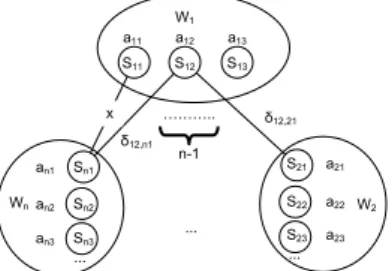
The objective (1) is quadratic, because it is the weighted sum of products of variable pairs (aij ·aij). To obtain an ilp problem, we introduce a binary variableδij,ij for each pair of sensessij, sij withi=i. Figure 1 illustrates the new formulation of the problem. Each one of the large circles, hereafter called
clouds, contains the possible senses (small circles) of a particular word occurrence wi. There must be exactly one active sense in each cloud. Each δij,ij variable shows if the edge that connects two sensessij andsij from different clouds is active (δij,ij = 1) or not (δij,ij = 0). We want an edge to be active if and only if both of the senses it connects are active (aij =aij = 1).
Fig. 1.Illustration of ourilp model of word sense disambiguation
The problem can now be formulated as follows, wherei, i∈ {1, . . . , n},i=i, and (i, j),(i, j) range over the indices of the possiblesij andsij, respectively.
maximize
i,j,i,j,i<i
rel(sij, sij)·δij,ij (3) such that aij ∈ {0,1}, ∀i, j and
j
aij= 1, ∀i (4)
δij,ij ∈ {0,1} and δij,ij =δij,ij, ∀i, j, i, j (5)
and
j
δij,ij =aij, ∀i, j, i. (6) The second constraint of (5) reflects the fact that the edges (and their activa-tions) are not directed. Constraint (6) can be understood by considering sepa-rately the possible values ofaij:
– Ifaij = 0 (sijis inactive),jδij,ij = 0, ∀i, i.e., all the edges that connect sij to the sensessij of each other word (cloud)wi are inactive, enforcing the requirement that any edge connecting an inactive sense must be inactive.
– Ifaij = 1 (sij is active), then jδij,ij = 1, ∀i, i.e., there is exactly one active edge connectingsij to the sensessij of each other word (cloud)wi. The active edge fromsij connects to the (single) active sense in the cloud ofwi, because if it connected to a non-active sense in that cloud, the edge would have to be inactive, as in the previous case. Hence, the active edge connects two active senses (from different clouds), as required.
An advantage of ilpsolvers is that they guarantee finding an optimal solution, if one exists. As already noted,ilpisnp-hard, but efficient solvers are available, and they are very fast when the number of variables and constraints is reasonably
small, as in our case.1We also implemented a pruning variant of ourilpmethod, which removes from the graph of Fig. 1 any sense sij whose WordNet gloss contains none of the other word occurrences being disambiguated; the pruning is not applied to the senses of word occurrences that would be left without any sense after the pruning. This pruning significantly reduces the number of candidate senses and, consequently, the execution time of our method.
3
Relatedness Measures
Lexical relatedness measures can be classified in three categories: (i) measures based on dictionaries, thesauri, ontologies, or Wikipedia hyperlinks, collectively called knowledge-based measures [4,14]; (ii) corpus-based measures, which use word or sense co-occurrence statistics, like pmi and χ2 [6,22]; and (iii) hybrid
measures [16,9]. Some measures are actually intended to assess the relatedness between words (or phrases), not word senses, but they can often be modified to work with senses. Other measures are intended to measure similarity, not relatedness, though the distinction is not always clear. The first measure that we adopt,SR, uses WordNet and belongs in the first category. The second measure is a hybrid one, since it uses both word co-occurrence statistics (to computepmi
scores) and WordNet’s glosses.
SR [20] requires a hierarchical thesaurusO with lexical relations, in our case WordNet, and a weighting scheme for lexical relations. Given a pair of senses s1, s2 and a path (sequence)P = p1, . . . , pl of senses connecting s1 = p1 to
s2 =pl via lexical relations, P’s “semantic compactness” (SCM) is defined as
below;wi→i+1are the weights of the lexical relations (sense to sense transitions)
ofP.2 The “semantic path elaboration” (
SPE) ofP is also defined below;di is the depth ofpi in O’s hierarchy, and dmax is the maximum depth ofO.
SCM(P) = l−1 i=1 wi→i+1 SPE(P) = l i=1 2didi+1 di+di+1 · 1 dmax
The semantic relatednessSRbetweens1ands2is defined below, whereP ranges
over all the paths connectings1tos2. If no such path exists, thenSR(s1, s2) = 0.
SR(s1, s2) = max
P=s1,...,s2{SCM
(P)·SPE(P)}
Instead ofSR(s1, s2), we useeSR(s1,s2), which leads to slightly better results.
For two wordsw1, w2, theirpmiscore isPMI(w1, w2) = log P (w1,w2)
P(w1)·P(w2), where
P(w1, w2) is the probability of w1, w2co-occurring (e.g., in the same sentence).
If w1, w2 are independent, their pmi score is zero. If w1, w2 always co-occur,
the score is maximum, equal to−logP(w1) =−logP(w2). With sense-tagged
1We use
lp solve; seehttp://lpsolve.sourceforge.net/.
2P is a path on WordNet’s entire graph, not the graph of Fig. 1 that we construct for each sentence. A Web service implementation ofSRwith precomputedSRscores for all WordNet senses is available; consult http://omiotis.hua.gr/.
corpora, thepmi score of two senses s1, s2 can be estimated similarly. In this
paper, however, where we do not use sense-tagged corpora, we use the WordNet glossesg(s1) andg(s2) ofs1 ands2, and the pmiscores of all word pairsw1, w2
fromg(s1) andg(s2), respectively, excluding stop-words:
PMI(s1, s2) =
w1∈g(s1), w2∈g(s2)PMI(w1, w2) |g(s1)| · |g(s2)|
Here|g(s)|is the length of g(s) in words. The intuition is that if s1 ands2 are
related, the words that are used in their glosses will also co-occur frequently. We use an untagged corpus of approx. 953 million tokens to estimatePMI(w1, w2).
4
Experimental Evaluation
We callilp-sr-fullandilp-sr-prunthe versions of ourilpmethod with and without sense pruning when theSRmeasure is used, andilp-pmi-fulland
ilp-pmi-prunthe versions with thepmi-based measure. We experimented with the
widely used Senseval 2 and 3 datasets, whose word occurrences are tagged with the correct WordNet senses. Both datasets have training and test parts.
We compare ourilpapproach against two other prominent unsupervisedwsd methods, both of which construct a large semantic graph for each input sentence. The graph has nodes not only for all the possible senses of the sentence’s words, but also for all the possible senses of the words that WordNet shows as related to the sentence’s words. The edges of the graph correspond to single lexical re-lations of WordNet. (Recall that, by contrast, our ilp approach constructs a much smaller graph for each sentence, which only contains nodes for the possi-ble senses of the sentence’s words; and the edges of our graph do not necessarily correspond to single WordNet lexical relations.) The first method we compare against, Spreading Activation Network (san), consequently applies a spreading activation to the semantic graph, and eventually retains the most active sense (node) of each word of the input sentence. We use thesanmethod of Tsatsaro-nis et al. [21], which is an improved version and, hence, representative of several othersanmethods forwsdgoing back to Quillian [15]. The second method we compare against, hereafter calledpr, applies PageRank on the semantic graph and retains the most highly ranked sense (node) of each word in the input sen-tence. PageRank was first used inwsdby Mihalcea et al. [8], but with different improvements it has also been used by others [2,19]. We use theprmethod that was recently evaluated by Tsatsaronis et al. [19]. Thesanandprmethods were chosen because they are well-known and implementations of both were available to us, unlike other unsupervisedwsdmethods [18,12,2].
When they cannot disambiguate (at all, or with high confidence) a word oc-currence, many unsupervised wsd methods resort to the first-sense heuristic, which selects the first sense of each word, as listed in WordNet. Te first sense is the most common one, based on frequencies from sense-tagged corpora; hence, the heuristic is actually a supervised baseline. Unfortunately, the heuristic on
Table 1.Coverage (C), precision (P), recall (R), and F1-measure (F) ofwsdmethods on the Senseval 2 and 3 datasets,polysemous words only, excluding adverbs,without using the first-sense heuristic. The results are percentages.
Senseval 2 Noun Verb Adjective All
Method C P R F C P R F C P R F C P R F san 72.2 27.8 20.0 23.3 71.1 19.6 13.9 16.3 72.4 39.6 28.7 33.3 71.9 27.9 20.0 23.3 pr 72.2 45.5 32.8 38.1 71.1 30.0 21.3 24.9 72.4 38.8 28.1 32.6 71.9 39.4 28.4 33.0 ilp-sr-full 99.6 38.6 38.4 38.5 99.6 25.0 24.9 24.9 92.8 37.4 34.7 36.0 98.1 34.2 33.533.8 ilp-sr-prun 99.6 38.6 38.4 38.5 99.6 24.6 24.5 24.5 92.8 37.7 35.0 36.3 98.1 34.1 34.433.8 ilp-pmi-full 99.6 27.9 27.7 27.8 98.9 23.4 23.2 23.3 100.0 37.9 37.9 37.9 99.5 28.6 28.4 28.5 ilp-pmi-prun99.6 28.6 28.5 28.6 98.9 24.7 24.5 24.6 100.0 43.5 43.5 43.5 99.5 30.5 30.4 30.5
Senseval3 Noun Verb Adjective All
Method C P R F C P R F C P R F C P R F san 97.9 30.6 29.9 30.2 94.2 28.8 27.1 27.9 94.9 37.8 35.9 36.8 95.8 31.0 29.7 30.4 pr 97.9 38.3 37.5 37.9 94.2 39.6 37.3 38.4 94.9 40.5 38.4 39.4 95.8 39.2 37.638.4 ilp-sr-full 99.9 32.3 32.2 32.3 98.0 25.8 25.3 25.6 97.0 38.3 37.1 37.7 98.6 30.6 30.2 30.4 ilp-sr-prun 99.9 32.0 31.9 32.0 98.0 25.8 25.3 25.6 97.0 38.7 37.5 38.1 98.6 30.5 30.1 30.3 ilp-pmi-full 96.7 30.2 29.2 29.7 94.1 18.1 17.1 17.6 96.9 39.4 38.2 38.8 95.7 26.9 25.8 26.3 ilp-pmi-prun96.7 27.3 26.4 26.8 94.1 19.3 18.2 18.7 96.9 39.0 37.8 38.4 95.7 26.1 24.9 25.5
its own outperforms all existing unsupervised wsd methods.3 Hence, the
ex-perimental results of most unsupervised wsdmethods, including ours, can be drastically improved by frequently invoking the first-sense heuristic, even for randomly selected word occurrences. We, therefore, believe that unsupervised
wsdmethods should not be allowed to use the heuristic in evaluations.
Table 1 lists the results of our experiments. We follow common practice and exclude adverbs. We consider only polysemous words, i.e., we ignore words with only one possible meaning (trivial cases), which is why the results may appear to be lower than results published elsewhere; the first-sense heuristic is also not used. Since all six methods may fail to assign a sense to some word occurrences, we show results in terms of coverage (percentage of word occurrences assigned senses), precision (correctly assigned senses over total assigned senses), recall (correctly assigned senses over word occurrences to be assigned senses), and F1
measure.4 A reasonable upper bound is human interannotator agreement [11]. For fine-grained sense inventories, like WordNet’s, interannotator agreement is between 67% and 80% [13]. A random baseline, assigning senses randomly with uniform probability, achieves approx. 20% and 14% accuracy on Senseval 2 and 3, respectively, counting both monosemous and polysemous words.
On the Senseval 2 dataset, the coverage of our ilpmethod (with both mea-sures, with and without sense pruning) was significantly higher than that ofsan 3When both monosemous and polysemous words are considered, the first-sense heuris-tic achieves 63.7% and 61.3% accuracy on the Senseval 2 and 3 datasets, respectively, with 100% coverage. At 100% coverage, precision and recall are equal to accuracy. 4We do not assign a sense to a word occurrence when the relatedness of all of its
andpr. In terms of F1-measure,ilp-sr-fullperformed overall better thansan
andpr, outperformingsanby a wide margin. Our method performed worse with thepmi-based measure (ilp-pmi-full) than withSR on the Senseval 2 dataset, though it still outperformed san, but not pr. The pruned versions (
ilp-sr-prun, ilp-pmi-prun) performed as well as or better than the corresponding
unpruned ones (ilp-sr-full,ilp-pmi-full), indicating that sense pruning suc-cessfully managed to remove mostly irrelevant senses. Sense pruning also leads to considerable improvements in execution time. The average execuation time per sentence (collectively on both datasets) was 82.81, 23.45, 81.46, 17.40 seconds for ilp-sr-full, ilp-sr-prun, ilp-pmi-full, ilp-pmi-prun, respectively. The corresponding times forsanandprwere 101.38 and 91.92, i.e., ourilpmethods are in practice faster than the implementations ofsanandprwe had available, even though the computational complexity of sanandpris polynomial.5
On the Senseval 3 dataset, the coverage of allilpmethods remains very high, with a small decline when thepmi-based measure is used. The F1 scores of the
ilpmethods are now lower, compared to their respective scores in Senseval 2; this is due to the larger average polysemy of Senseval 3 (8.41 vs. 6.48 for polysemous words). Surprisingly, however,sanandprnow perform better than in Senseval 2; andproutperforms ourilpmethods , with the overall difference betweensan
andilp-sr-fullnow being negligible. We can only speculate at this point that the improved performance ofsanandprmay be due to the higher polysemy of Senseval 3, which allows them to construct larger graphs, which in turn allows them to assign more reliable rank or activation scores to the nodes (senses). The coverage ofsanandpris also now much higher, which may indicate that as their graphs become larger, it becomes easier forsanandprto construct connected graphs; both methods require a connected graph, in order to rank the nodes or spread the activation, respectively. Also, the prunedilpmethods now perform worse than the corresponding unpruned ones, indicating that sense pruning is less successful in discarding irrelevant senses as polysemy increases.
We aim to investigate the differences between the Senseval 2 and 3 results further in future work. For the moment, we conclude that ourilpapproach seems to work better with lower polysemy. We believe, though, that our experiments againstsanandpr already show the potential of ourilpmodel.
5
Conclusions
We presented anilpmodel of wsd, which can be used with off-the-shelf solvers and any sense relatedness measure. We experimented withSRand a hybridpmi -based measure on the Senseval 2 and 3 datasets, against two well-known methods based on PageRank (pr) and Spreading Activation Networks (san). Overall, our
ilpmodel performed better with SR. With that measure, it performed better
than bothprandsanon the Senseval 2 dataset, outperforming sanby a wide margin. By contrast,pr performed much better than our ilp methods on the
5The complexity of
sanis O(n2·k2l+3), and pr’s is O(n2·k32l+3), where k is the maximum branching factor of the hierarchical thesaurus, l its height, and n the number of word occurrences to be disambiguated [19].
Senseval 3 dataset, and the difference between san and our best ilp method was negligible. In practice, our ilp methods run faster than the pr and san
implementations we had available. We hope that ourilpmodel will prove useful to others who may wish to experiment with different relatedness measures.
References
1. Agirre, E., Lopez de Lacalle, O.: Supervised domain adaption for word sense dis-ambiguation. In: EACL (2009)
2. Agirre, E., Soroa, A.: Personalizing PageRank for word sense disambiguation. In: EACL (2009)
3. Florian, R., Cucerzan, S., Schafer, C., Yarowsky, D.: Combining classifiers for word sense disambiguation. Natural Language Engineering 8(4), 327–341 (2002) 4. Gabrilovich, E., Markovitch, S.: Computing semantic relatedness using
Wikipedia-based explicit semantic analysis. In: IJCAI (2007)
5. Lesk, M.: Automated sense disambiguation using machine-readable dictionaries: How to tell a pine cone from an ice cream cone. In: SIGDOC (1986)
6. Manning, C., Schutze, H.: Foundations of Statistical NLP. MIT Press (2000) 7. Mihalcea, R., Csomai, A.: SenseLearner: Word sense disambiguation for all words
in unrestricted text. In: ACL (2005)
8. Mihalcea, R., Tarau, P., Figa, E.: PageRank on semantic networks with application to word sense disambiguation. In: COLING (2004)
9. Montoyo, A., Suarez, A., Rigau, G., Palomar, M.: Combining knowledge-and corpus-based word-sense-disambiguation methods. JAIR 23, 299–330 (2005) 10. Navigli, R.: Online word sense disambiguation with structural semantic
intercon-nections. In: EACL (2006)
11. Navigli, R.: Word sense disambiguation: A survey. ACM Computing Surveys 41(2), 10:1–10:69 (2009)
12. Navigli, R., Lapata, M.: Graph connectivity measures for unsupervised word sense disambiguation. In: IJCAI, pp. 1683–1688 (2007)
13. Palmer, M., Dang, H., Fellbaum, C.: Making fine-grained and coarse-grained sense distinctions, both manually and automatically. NLE 13(2), 137–163 (2007) 14. Ponzetto, S., Strube, M.: Knowledge derived from Wikipedia for computing
se-mantic relatedness. J. of Artificial Intelligence Research 30, 181–212 (2007) 15. Quillian, R.: The teachable language comprehender: a simulation program and
theory of language. Communications of ACM 12(8), 459–476 (1969)
16. Resnik, P.: Using inform. content to evaluate semantic similarity. In: IJCAI (1995) 17. Sch¨utze, H.: Automatic word sense discrimination. Computational
Linguis-tics 24(1), 97–123 (1998)
18. Sinha, R., Mihalcea, R.: Unsupervised graph-based word sense disambiguation us-ing measures of word semantic similarity. In: IEEE ICSC (2007)
19. Tsatsaronis, G., Varlamis, I., Nørv˚ag, K.: An Experimental Study on Unsupervised Graph-based Word Sense Disambiguation. In: Gelbukh, A. (ed.) CICLing 2010. LNCS, vol. 6008, pp. 184–198. Springer, Heidelberg (2010)
20. Tsatsaronis, G., Varlamis, I., Vazirgiannis, M.: Text relatedness based on a word thesaurus. JAIR 37, 1–39 (2010)
21. Tsatsaronis, G., Vazirgiannis, M., Androutsopoulos, I.: Word sense disambiguation with spreading activation networks generated from thesauri. In: IJCAI (2007) 22. Turney, P.D.: Mining the Web for Synonyms: PMI-IR versus LSA on TOEFL.
In: Flach, P.A., De Raedt, L. (eds.) ECML 2001. LNCS (LNAI), vol. 2167, pp. 491–502. Springer, Heidelberg (2001)