Georg Schollmeyer, Thomas Augustin
On Sharp Identification Regions for Regression Under
Interval Data
Technical Report Number 143, 2013
Department of Statistics
University of Munich
Abstract
The reliable analysis of interval data (coarsened data) is one of the most promising applications of imprecise probabilities in statistics. If one refrains from making untestable, and often materially unjustified, strong assumptions on the coarsening process, then the empirical distribution of the data is imprecise, and statistical models are, in Manski’s terms, partially identified. We first elaborate some subtle differences between two natural ways of handling interval data in the dependent variable of regression models, distinguishing between two different types of identifi-cation regions, calledSharp Marrow Region (SMR)andSharp Collection Region (SCR)here. Focusing on the case of linear regression analysis, we then derive some fundamental geometrical properties of SMR and SCR, allowing a comparison of the regions and providing some guidelines for their canonical construction.
Relying on the algebraic framework of adjunctions of two mappings be-tween partially ordered sets, we characterize SMR as a right adjoint and as the monotone kernel of a criterion function based mapping, while SCR is indeed interpretable as the corresponding monotone hull. Finally we sketch some ideas on a compromise between SMR and SCR based on a set-domained loss function.
This paper is an extended version of a shorter paper with the same ti-tle, that is conditionally accepted for publication in the Proceedings of the Eighth International Symposium on Imprecise Probability: Theories and Applications. In the present paper we added proofs and the seventh chapter with a small Monte-Carlo-Illustration, that would have made the original paper too long.
Keywords:partial identification, imprecise probabilities, interval data, sharp identification regions, coarse data, adjunctions, partially ordered sets, linear regression model, best linear predictor, set-domained loss func-tion.
1
Introduction
The methodology of imprecise probabilities offers powerful methods for reliable handling of coarse(ned) data, see, e.g., the ISIPTA contributions by [18, 44, 40, 37, 41, 7, 20]. The term coarsened data, or epistemic data imprecision, is an umbrella term, comprising all situations where data are not observed in the resolution intended in the subject matter context. This means, there is a certain true precise valuey∈ Yof a generic variableY of material interest, but we only observe a setA⊇ {y}. An extreme special case of coarse data aremissing data, where the missingness of valueyiof unitican be interpreted as having observed
the whole sample spaceY. In the case whereAis an interval [y,y] for y,y∈R coarse data are commonly calledinterval data.
Before turning to the formal framework, two issues with fundamental im-portance for practical applications shall be recalled.
First of all, it must be stressed that the term ‘coarse’ is a relative term. Whether data are coarse or not depends on the specified sample space, and therefore on the subject matter context to be investigated. If, for instance, the sample space is taken to consist of some a priori specified ranges for income data, and that is all what is needed, then data are not coarse, while if precise income values are of interest, the data are coarse.1
Secondly, it is important to emphasize that coarse data typically are not just the result of sloppy research, like an insufficient study design or improper data handling. On the contrary, coarse data are an integral part of data collec-tion, in particular in social surveys. Interval data arise naturally from the use of categories in order to avoid refusals in the case of sensitive questions, and are a means to model roughly rounded responses (see, e.g., [24]). Coarsened categorical data are, for instance, produced by matching data sets with not fully overlapping categories, are the direct outcome of data protection by some anonymization techniques (see, e.g., [13]), or may be produced by the combina-tion of spaces with given marginals by Frech`et bounds (see, e.g., [19]). Another prototypic setting is the case of systematically missing data, arising from treat-ment evaluations in non-randomized designs like observational studies.2
By confining themselves to precise probabilities, traditional statistical approaches to cope with coarse data are inevitably forced to try to escape the imprecision in the data eventually. An immediate way in the case of interval data [yi, yi]
for each unit i= 1, . . . , nin the sample is to replace each interval by the cor-responding central value ˚yi= (yi+yi)/2, and then to proceed with a standard
analysis based on that fictitious sample. More sophisticated approaches add complex, typically untestable assumptions, either to explicitly model the coars-ening process by a precise model, or to characterize idealized situations where the coarsening can be included in standard likelihood and Bayesian inference without biasing the analysis systematically.3
In recent years, awareness in statistics and econometrics has grown that such strong assumptions quite often cannot be justified by substantive arguments, and thus the – too high – price for the seemingly precise result of the statistical analysis is the loss of credibility of the conclusions, and in the end
consequen-1Indeed, even unions of intervals may constitute precise observations, for instance as the response to the question ‘When did you live in Munich?’, measured in years. Then
{[1986; 1991]∪[1997; 2000]}is a precise observation in the sample space of all finite unions of closed intervals [a, b] witha, b∈N+. (See in particular the distinction betweenconjunctive
anddisjunctiverandom sets in [14, Section 1.4], from which also this example is adopted.) 2To evaluate effects of treatment or interventionAover treatmentB, in principle, it would be necessary to have information from a parallel universe, so-to-say, i.e. to know in addition how the units treated withAwouldhave reactedifthey had been given the treatmentBand vice versa.
This question has in particular attracted intensive attention in the partial identification liter-ature in econometrics (see, for instance, the survey [39] or the instructive case study [36].
3Most prominent is here Little and Rubin’s [22] classification, distinguishing situations of
missingness completely at random (MCAR)ormissing at random (MAR)frommissing not at random (MNAR)settings, where a systematic bias has to be expected. This classification has been extended to coarsening by [16].
tially the practical relevance of the statistical analysis.4 In the light of this, it
is of particular importance to develop approaches that reflect the underlying imprecision in the data properly, resulting in potentially imprecise, but reliable results. The fascinating insight, corroborated by a variety of applications mainly in econometrics (see the exemplary references below), is that in many studies these results are still enough to answer important substantive science questions, and if not, the scientist is alerted that strong conclusions drawn from the data may be mere artefacts.
Related approaches, considering all possible data compatible with the observed set of values, have been developed almost independently in different settings, ranging from reliable computing and interval analysis in engineering (e.g., [29]) and extensions of generalized Bayesian inference [10, 45] to reliable descriptive statistics in social sciences ([32, Chapter 17f], [30]). This cautious way to pro-ceed is closely related to set-based (profile-)likelihood approaches ([47, 7]) and to the methodology of partial identification, in particular propagated by Man-ski (e.g., [23]) in econometrics, and to systematic sensitivity analysis (e.g. [42]) in biometrics, where a general framework for imprecise data models, i.e. sets of observationally equivalent statistical models, has been developed. In these models instead of single valued parameters one obtains so-calledidentification regions, i.e. sets of all parameters compatible with the data. On the inferen-tial side, there has been important progress in the development of appropriate confidence procedures (see, e.g., [5, 27, 6]), and computational techniques have maturated to the extent that routine use of basic procedures has become feasible (e.g., [8, 1, 38, 33]). As a result, applied contributions are now rather common and are particularly influential in econometrics and allied fields see, e.g., [28] for an analysis of income poverty measures based on coarsened survey data, [21] for a study of the German reform of unemployment compensation based on register data and [26] for an analysis of treatment effects in observational studies with an illustration based on the National Longitudinal Survey of Youth.
The paper is organized as follows. After some basic definitions (Section 2), we emphasize in Section 3 the distinction between different understandings and goals of regression models, leading to two different types of identification regions, called SMR and SCR here. Section 4 formulates some basic geometrical properties, while sections 5 applies an algebraic framework for investigating mappings between partially ordered sets. We recall the basic concepts needed here, and explain them exemplary in the context of Dempster-Shafer-Theory and by describing coherent lower previsions as hulls. Then SMR and SCR are characterized as the monotone kernel and monotone hull of a criterion function based mapping, respectively. Section 6 suggests another type of identification regions that is based on a strict set-valued perspective, relying on a loss function depending on sets of parameters. Section 7 illustrates all the three identification regions and the predictions made by these regions while Section 8 concludes.
2
Basic Definitions
Let Θ be a parameter space andP := {Pθ |θ ∈Θ} a corresponding
statisti-cal model on a measurable space (Ω,F) with the associated observable random variablesX,Y,Y and the unobserved random variableY. We are interested in the relationship betweenX andY, but we have no full information aboutY, we only know that the unobserved variableY is related to the observed Y and Y in the sense thatY fulfills a certain relation, for exampleP(Y≤Y ≤Y) = 1 or E(Y|X)≤E(Y |X)≤E(Y|X)5. In the sequel, we assume the second
condi-tion with the addicondi-tional assumpcondi-tion thatE(Y|x) andE(Y|x) are continuous inx. WithPwe denote the unknown true model and withEthe corresponding expectations. The expectations for a modelPθ are denoted withEθ. The joint
distribution of the random variables X, Y,Y,Y under a model Pθ is denoted
withFθX,Y,Y,Y(or shortFθ) and the joint distribution under the true modelPis
denoted withFX,Y,Y,Y(or shortF). Analogously, the distribution of a subset of
random variables, eg. {X, Y}is denoted withFθX,Y andFX,Y respectively. For
arbitrary random variables like e.g. X, Z,Y,Y we denote their joint distribution with FX,Z,Y,Y. BecauseY is not observable, we have not the full information
aboutY, which generally leads to partially identified models, which we define in the sequel: Two parametersθ1,θ2∈Θ are undistinguishable (i.e. θ1∼θ2) if
the corresponding modelsPθ1 andPθ2 are empirically undistinguishable, which
means that the distributions of the observable variables are the same. A statis-tical modelP is calledpoint-identified, if any two different parametersθ1and
θ2are empirically distinguishable. Otherwise it is calledpartially identified.
Example 1 The simple linear model with interval outcomes:
Θ =B×R
withB=R2the actually interesting parameter space andR=RΩ×RΩ
≥0×RΩ≥0
describing the error-terms and the coarsening-process: For θ= (β,(ε, δl, δu))∈
Θ the associated variables are defined as
Y = Xβ+ε, Y = Xβ+ε−δl
Y = Xβ+ε+δu
with ε, δl, δu measurable andε with existing conditional expectationsE(ε|x) =
0. The coarsening process is modeled by the random variablesδl andδuthat are
nonnegative, which ensures Y≤Y ≤Y. By abuse of notation we identify the random variable X with the matrix (1, X) to use matrix notations like above, if useful. Furthermore, in the sequel we assume X as a fixed random variable with support R and therefore omit it in the parameter space Θ. It is clear that this model is only partially identified. For example ((β0, β1),(ε,0,1)) ∼
((β0+ 1, β1),(ε,1,0)). Moreover, the quotient space Θ/∼ is not of the form
Θ/∼=B/∼B×R/∼R for some relations∼B and∼R, so we must factorize the
whole space Θ and not only the interesting part B to make the model point-identified.
3
Two Types of Identification Regions
There are two ideal type senses of what a statistical model is and what it should render. One can assume a statistical model as the exact true underlying prob-abilistic structure, from which one only has to know all details and then one knows the exact distributions of all involved random variables and can make inferences with this knowledge. In contrast one can see a statistical model not as a truth, but as a rough approximation of truth and use it as a parsimonious tool to predict for example future observations of some variables or to get a rough insight into the real underlying structure that is actually more complex. As examples for this differentiation one could see firstly the estimation of the intercept and the slope of a linear model and secondly the problem of finding the best linear predictor in the sense of [2], which makes predictions that are linear in the covariates, but the underlying model needs not to be linear. The main difference is here that in the first case we really assume a linear model and rely on it, whereas in the second case we use the linearity of the predictions only to have a parsimonious model for predictions or explanations, but we assume nothing about the true statistical model.
These views lead to different problem formulations, which we want to state now as we need it in our context. In order to efficiently tackle our goal, we leave the statistical perspective and join Manski ([23, p. 7]), who recommends that problems of identification become much clearer when one firstly separates non-identifiability from sample variation, and assumes all distributions to be known for the analytic treatment6 (later on then sample counterparts may be
constructed in the usual way). In particular, we also assume that the distribu-tion ofY is known (and we have no variables Y and Y) and later we generalize this to the case of an unobservedY, which leads to different sharp identification regions that are then our objects of interest.
The first problem statement is: Given the distributionFX,Y of (X, Y), which
is an element of the class{FθX,Y |θ∈Θ}, find allθ, such that (X, Y)∼FθX,Y, which is equivalent to find all θ with L(FθX,Y, FX,Y) = 0 for an arbitrary
distance-functionL(·,·) or a similar function, which is zero if and only if both arguments are equal. Here we think of a kind of loss function and introduce this equivalent formulation to indicate the analogy to the second problem formula-tion:
Given the distributionFX,Y, which is an element of the class{FX,Y θ |θ∈
Θ}, find all θ, such that L(FθX,Y, FX,Y) is minimal. In contrast to the first 6The identification regions arising in this limit case are calledsharpidentification regions.
problem, this problem definition is also meaningful if FX,Y ∈ {/ FX,Y
θ |θ∈Θ},
i.e. if the model is not correctly specified. If the model is correctly specified, then both problems are often essentially the same in the sense that for example for a linear model, the BLUE-estimator and the best linear predictor (with a quadratic loss-function) are solving different tasks, but the parameter estimates are identical. The actual problem is now thatFX,Y is unknown. One part of
the problem is that also if we could observe Y, we could not know the exact distribution ofY and so we have to estimate it. In particular, we cannot decide with certainty, if FX,Y is an element of the class {FX,Y
θ |θ ∈Θ}, and so the
two problem formulations are moving together a little bit. The other part of the problem is that the variableY, we are actually interested in, is not observable. As argued above for the moment we only address this second part of the problem and assume that we know the exact distribution of all observable variables. Later in section 5.2 we also address the other part. If now Y is unobserved, we can generalize the two problems by applying them to all possible Y that are consistent with (Y,Y).This leads to different regions of parameters that were proposed in different papers: The region related to the first problem was introduced slightly differently in [9] and the other region was proposed as the sharp identification region for the best linear predictor in [2].
Definition 1 LetP ={Pθ|θ∈Θ}be a statistical model with the corresponding
joint distributions{FθX,Y |θ∈Θ}andX,Y,Ygiven random variables. (i) The sharp marrow region (SMR)is defined as:
SM R:={θ∈Θ|E(Y|X)≤Eθ(Y |X)≤E(Y|X)}.
Note that theY in the definition is the Y coming from the modelPθ, not
theY from the true model. If the model is correctly specified (or if at least
SM R6=∅), this region can also be written as:7
SM R= argmin θ∈Θ " min Z∈E([Y,Y]|X)L FθX,Y, FX,Z, #
with an arbitrary loss function L. Here with E([Y,Y] | X) we denote the set of all random variables Z fulfilling E(Y | X) ≤ E(Z | X) ≤
E(Y | X). This equivalent characterization of SM R is valid because a parameterθ∈Θis inSM Rif and only if there exists aZ∈E([Y,Y]|X)
with Fθ=FX,Z,Y,Y or equivalently L(Fθ, FX,Z,Y,Y) = 0. From the above
representation of SMR we can see that SMR can be written as the solution of a decision problem with a minimin decision rule.
(ii) Thesharp collection region (SCR)is defined as:
SCR:= [ Z∈[Y,Y] argmin θ∈Θ LFθ, FX,Z,Y,Y .
With [Y,Y] we denote the set of all random variablesY that lie between
Yand Yfor allω∈Ω.
A first comparison of this two regions that emphasizes the case of misspecifica-tion and interpretamisspecifica-tional problems for the sharp marrow region in this case can be found in [31]: While the interpretation of the sharp collection region as the collection of all best linear predictors is clear, the interpretation of SMR seems to be not so useful under misspecification, especially if SMR is empty.8 From
an empty SMR we can conclude, that the model is misspecified, but not more. Furthermore in the above-mentioned paper the authors make clear that a tight SMR “cannot be viewed as an indicator that the underlying model contains a lot of information about the true but partially identified parameter.”9. An
illustration of these considerations, that we pick up in chapter 7 can also be found in [31].
4
Geometrical Properties of Identification
Re-gions
From now on, we concentrate on the case of a linear model like in example 1 and the classical quadratic loss function. Since we are only interested in the components (β0, β1) of an elementθ = ((β0, β1),(ε, δl, δu)) ∈SM R, by abuse
of notation, we also denote the set{(β0, β1)|((β0, β1),(ε, δl, δu))∈SM R} as
the sharp marrow region (analogously for the sharp collection region). Then we have
SM R = β∈B|E(Y|X)≤Xβ≤E(Y|X) and SCR = {argmin
β∈B E
((Xβ−Y)2)|Y ∈[Y,Y]}.
Remark 4.1 The sharp marrow region is always a subset of the sharp collection region, and this is the reason for calling it sharp marrow region, it is the marrow of all truly linear models that fit to some Z ∈ [Y,Y]. In contrast, the sharp collection region collects the best fitting parameters for every possibleZ∈[Y,Y].
Proof: With β ∈ SM R we have E(Y | x) ≤ xβ ≤ E(Y | x) for all x and therefore we can choose Y(x) := λ(x) Y +(1−λ(x)) Y withλ(x) ∈ [0,1] such that
E(Y |x) =xβ. It is clear thatY ∈[Y,Y] and withε:=Y−Xβwe getE((Xβ−Y)2) = E((Xβ−Xβ+ε)2) = E(ε2) and for all further ˜β ∈ R2 we have E((Xβ˜−Y)2) = E((Xβ˜−Xβ+ε)2) =E((Xβ˜−Xβ)2) +E(ε)2+E(2(Xβ˜−Xβ)·ε)≥E(ε2), since all
conditional expectations ofεare zero. Thus we have shownβ∈SCR.
It is easy to see that the sharp marrow region is convex and closed. Further-more, all convex, compact sets can be represented as a sharp marrow region:
8But compare the remarks in the next to last paragraphs of chapters 5.1 and 5.2. 9[31, p. 202].
Proposition 4.1 LetI ⊂R2be a compact convex set. Then there exist random
variablesY,Y such thatSM R(Y,Y) =I, namely:
Y = min{Xβ|β∈I}
Y = max{Xβ|β∈I}.
Proof: From β ∈ I it follows E(Y | X) = Y ≤ Xβ ≤ Y = E(Y | X), which means that β is in SM R(Y,Y). If β /∈ I because of the separation lemma (see e.g. [17]), there exists a linear functional onR2, represented by a vector (x
0, x1) with x0β0+x1β1< inf β∈Ix0β0+x1β1. Ifx0>0 it followsβ0+ x1 x0β1<βinf∈Iβ0+ x1 x0β1= Y( x1 x0),
which shows thatβ /∈SM R(Y,Y). Forx0= 0 we havex1β1< inf
β∈Ix1β1, which leads
toβ0+nx1β1< inf
β∈Iβ0+ infβ∈Inx1β1≤βinf∈Iβ0+nx1β1= Y(nx1) ifnis large enough.
The casex0<0 can be proved analogously to the casex0>0.
For the sharp collection region, the situation is more complicated. To analyze this, we need some definitions from geometry (cf. [46]):
Definition 2 The Minkowski sum
M = n M i=1 li= ( n X i=1 pi pi∈li )
ofnline segmentsli⊆Rdis called azonotope. A zonotope is a convex, compact and centrally symmetric polytope with finite many extreme points and centrally symmetric facets. A closed, centrally symmetric convex setZ ⊆Rdis called a zonoidif it can be approximated arbitrarily closely by zonotopes (w.r.t. a metric, e.g. the Hausdorff distance). For d= 2the zonoids are exactly the closed, centrally symmetric convex sets (see, e.g., [3]).
Proposition 4.2 LetE(Y),E(Y),E(Y·X),E(Y·X)be finite and Var(X)6= 0. Then the sharp collection region is a zonoid.
Proof: The estimatorSCRˆ :={(x0x)−1x0y|y∈[y,y]}forSCRproposed in [2] is, as the linear image of a cuboid, a zonotope (see [8, p. 36]). Since (, as shown in [2, p. 784])SCRˆ is a consistent estimator of SCR with respect to the Hausdorff distance, it is clear that every sharp collection region is a limit object of zonotopes, thus a zonoid.
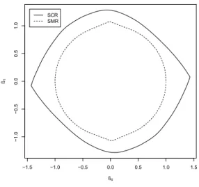
Now, the question arises, if every zonoid can be represented as a sharp collection region. At first glance this seems to be not the case. By looking at examples of (estimates of) sharp collection regions, like that in figure 1 one observes that this regions often have two points on its boundary at which the boundary is not smooth. Note that the situation for SMR is similar, if X has finite or compact support. If the separating functional of the proof of Proposition 4.1 has x0= 0, the argumentnx1of Y(nx1) could have such a high absolute value that
this value only occurs with probability zero, which leads to similar unsmooth situations, see figure 1. Fortunately one can prove that every zonotope Z in
−1.5 −1.0 −0.5 0.0 0.5 1.0 1.5 −1.0 −0.5 0.0 0.5 1.0 ß0 ß1 SCR SMR
Figure 1: SCR and SMR with unsmooth boundary
general position (and, by looking on suitable limit-processes, also every zonoid) can be represented as a sharp collection region if we define the distribution of X,Y and Y in a certain way10.
Proof: Without loss of generality, we have a zonotopeZ generated byn line-segments that start in the origin of coordinates and have lengthdiand slopesi. With
general position, we mean si< ∞. Now fori= 1, . . . , n takexi :=si,yi = 0,yi= di
√
1+x2
i
and add further xn+1, . . . , xmsuch that (m1x0x) =
1 ¯x ¯ x x¯2 = 1 0 0 1 and y n+1 =. . .= ym= yn+1 =. . .= ym= 0. Then we haveSCRˆ ={(x 0x)−1x0y| y∈[y,y]}= 1 m Py i P xiyi |y∈[0,y]
which is exactly the Minkowski addition of
nline segments with slopexi=siand length m1
p y2 i +x2iyi2= yi m p 1 +x2 i =di.
The last question is now, how independently from each other the regions SMR and SCR can be generated.
Proposition 4.3 LetI=SCR(Y∗,Y∗)⊆R2be a zonoid andE⊆SM R(Y∗,Y∗)
an arbitrary compact convex set. Then for everyε >0there exist random vari-ables Y,Y such that:
d(SCR(Y,Y), I) ≤ ε d(SM R(Y,Y), E) ≤ ε,
10The main difference to SMR is that there we could construct regions for every arbitrary
wheredis a metric on subsets ofR2, e.g. the Hausdorff distance.
Proof: Forε >0 define S ⊆R such that the distance from any pointxtoS and the distance from xtoSC andP(X ∈S) tends to zero asε goes to zero. Then set
(Y,Y) to (Y∗,Y∗) if x∈SC and ifx∈S set (Y,Y) to the random variables (Z,Z)
that generate E. Then SM R((Y,Y))−→SM R((Z,Z)) = EandSCR((Y,Y))−→
SCR((Y∗,Y∗)) =I.
5
An Algebraic View on Identification Regions
In the next section, we want to look at SMR and SCR as mappings. To analyze the algebraic structure of these mappings, we need some facts about adjunctions. Adjunctions arise in many contexts and often make life a bit easier, see the next examples. For an introduction to partially ordered sets and adjunctions see, e.g., [11, 15].Definition 3 Let(P,≤)and (Q,v)be partially ordered sets. A pair (f, g) of mappings f:P −→Q andg:Q−→P is calledadjunction, if:
∀p∈P∀q∈Q: p≤g(q) ⇐⇒ f(p)vq.
In this case, f is calledleft adjointandg is calledright adjoint.
Lemma 5.1 Let(f, g)be an adjunction. Then the following holds: A1 g◦f is extensive andf◦g is intensive, i.e.:
∀p∈P, q∈Q:g(f(p))≥p & f(g(q))vq. A2 f and gare order-preserving (monotone).
A3 f◦g◦f =f andg◦f◦g=gand thus f◦g andg◦f are idempotent. A4 From A1 - A3 it follows that g◦f is a closure operator and f◦g is a
kernel operator.11
A5 The adjoints f and gare determining each other unambiguously. A6 f preserves existing joins andg preserves existing meets.
To illustrate the concept of adjunctions, we apply it to two areas of the theory of imprecise probability.
Example 2 Dempster-Shafer-Theory12:
In [12] we have the multivalued mapping Γ : X −→ 2S with which we can
associate a set-domained version
˜
Γ : (2X,⊆)−→(2S,⊆) :A7→ [ a∈A
Γ(a).
11A closure operator is a monotone, extensive and idempotent mapping and a kernel oper-ator is a monotone, intensive and idempotent one.
Furthermore we have the operator
∗: (2S,⊆) −→ (2X,⊆) :
T 7→ T∗:={x∈X |Γ(x)⊆T}.
Then it is obvious that the pair(˜Γ, ∗)is an adjunction because bothA⊆T∗ and
˜
Γ(A)⊆T are meaning exactly that all a∈Aare mapped to subsets ofT. From this, the∞-monotonicity of a belief functionB =P ◦ ∗ with P a
probability-measure follows immediately, sinceP is∞-monotone and ∗is meet-preserving:
B(Sk i=1 Ti) =P(( k S i=1 Ti)∗)≥P( k S i=1 (Ti)∗) ≥ P J6=∅ (−1)|J|+1P(T i∈J (Ti)∗)=P J6=∅ (−1)|J|+1P((T i∈J Ti)∗) = P J6=∅ (−1)|J|+1B(T i∈J Ti).
Furthermore, it is clear that also the composition of a belief function and∗or another meet-preserving mapping is∞-monotone.
Example 3 Lower Coherent Previsions13:
With (RL(Ω),≤) the set of all previsions that are defined on all gambles and
avoid sure loss, equipped with the dominance relation P1 ≤ P2 : ⇐⇒ ∀X ∈
L(Ω) :P1(X)≤ P2(X)and (2P(Ω),⊇)the set of all nonempty sets of finitely
additive probability-measures on Ωwith the ordinary superset relation, we can construct the following adjunction:
f : (RL(Ω),≤) −→ (2P(Ω),⊇) :P 7→ M(P) g: (2P(Ω),⊇) −→ (RL(Ω),≤) :M 7→PM
with M(P) = {p ∈P(Ω)| ∀X ∈ L(Ω) : p(X)≥ P(X)}, where P(Ω)is the set of all finitely additive probability-measures and PM : L(Ω) −→ R : X 7→
inf
p∈Mp(X). In this language, because of the lower envelope theorem
14 coherent
lower previsions are exactly the hulls15of the closure operatorg◦f, which maps
a lower prevision that avoids sure loss to its natural extension. It is now easy to see that the natural extension of a prevision P is the lowest coherent prevision that dominates P: If P2 ≥ P is another coherent prevision that dominates
P, then it is a hull (g◦f)(Q)for some Q and with the idempotence and the monotonicity ofg◦f we have P2= (g◦f)(Q) = (g◦f◦g◦f)(Q)≥(g◦f)(P),
where the right hand side is the natural extension of P.
13For an introduction, see [43]. 14See [43, p. 134].
15Hulls are the images of a closure operator and similarly kernels are the images of a kernel operator.
5.1
SMR as a Right Adjoint
Proposition 5.2 Let (Y,≤) be the set of pairs of numeric random variables
Y= (Y,Y), equipped with the relation≤ defined by
Y1≤ Y2: ⇐⇒ E(Y1|X)≤E(Y2|X) &
E(Y1|X)≥E(Y2|X).
This means that if Y1 ≤ Y2, the observable variables (Y1,Y1)are more
infor-mative than(Y2,Y2)or equally informative, because from(Y1,Y1)we can learn
more or the same about the conditional expectations of the unobserved variable
Y, we are actually interested in. The mapping
SM R: (Y,≤) −→(2B,⊆) :
(Y,Y) 7→ {β|E(Y|X)≤Xβ≤E(Y|X)}
is a right adjoint. The corresponding left adjoint is the prediction-operator16:
P R: (2B,⊆) −→ (Y,≤) : Γ 7→ inf
β∈ΓXβ,supβ∈ΓXβ
!
.
Proof: We show Γ⊆ SM R(Y) ⇐⇒ P R(Γ) ⊆ Y: ⇒: LetZ = (Z,Z) :=P R(Γ) and Y = (Y,Y)). Then we have Z(x) = inf
β∈Γxβ ≥ β∈SM Rinf(Y)xβ ≥ E(Y | x) and Z(x) = sup β∈Γ xβ≤ sup β∈SM R(Y) xβ≤E(Y|x).
⇐: Letβ∈Γ. We have to showβ∈SM R(Y) or equivalently∀x:E(Y|x)≤xβ≤
E(Y|x):
xβ≤sup
β∈Γ
xβ≤E(Y|x) andxβ≥ inf
β∈Γxβ≥E(Y|x).
BecauseSM R is a right adjoint, it has the propertiesA1−A6. The mono-tonicityA2 means that SM R(Y) is more informative ifY is more informative. The idempotenceA3 means that if we estimate, predict and then estimate again, we get the same information as if we had only estimated one time. Analogously if we predict, estimate and then predict once more, we get the same prediction as we would get, if we predicted only once. This property is often satisfied by classical estimators, for example the classical least squares estimator has an idempotent prediction matrix. BecauseP R◦SM Ris a kernel operator, we can now give a clear interpretation ofSM R, which is also valid in the misspecified case: The sharp marrow region is the largest region for which the correspond-ing predictions constitutes the largest inner approximation of the conditional expectations17. This interpretation may be not so useful in the misspecified
situation, but it is clearly stated. The monotonicity is also shared by SCR,
16Here, the empty infimum is defined as∞and the empty supremum is defined as−∞. 17An empty SMR means, that there is no inner approximation induced by the prediction of a set of parameters.
but SCR is no right adjoint, since it is not meet-preserving, because the inter-section of two zonoids is generally not a zonoid. Furthermore, generally only (SCR◦P R◦SCR)(Y)⊃SCR(Y) holds, which means that we generally loose information if we predict and estimate once more.
5.2
SMR and SCR as a Kernel and a Hull
In [9] a criterion function based identification region is proposed. The criterion function (see Prop. 5.3) is based on a generalization of the expected squared errors to the expected squared minimal errors. The proposed sharp identification region is the argmin of this criterion function and it is very similar to SMR, but it is not monotone. It shows up that SMR is the highest lower and SCR is the lowest upper monotone approximation of this region.
Definition 4 LetE : (P,≤)−→ (Q,v)be a mapping. The monotone hull of
E is defined as:
H(E) : (P,≤)−→(Q,v) :X7→ _ Y≤X
E(Y).
The monotone kernel ofE is defined as:
K(E) : (P,≤)−→(Q,v) :X 7→ ^ Y≥X
E(Y).
These set-valued mappings are both order-preserving. Furthermore, the mapping
E 7→ H(E) is a closure operator and the mapping E 7→ K(E) is a kernel operator, thus indeedH(E)is a hull andK(E)is a kernel. In particular,H(E)
is the lowest order-preserving mapping that is higher thanE. Analogously,K(E)
is the highest order-preserving mapping that is lower thanE.
Proposition 5.3 Let the criterion function
Q:B→Rbe defined as Q(β) = Z (E(Y|x)−xβ)2++ E(Y|x)−xβ2−dP(x) = Z min Y∈[Y,Y](E(Y |x)−xβ) 2dP(x).
Then the criterion function based mapping
EQ: (Y,≤) −→ (2B,⊆) :
(Y,Y) 7→ argmin
β∈B
Q(β)
is a source of SMR and SCR:
Proof: First, we mention that SCR is the monotone hull of the ordinary least squares estimator defined asOLS: (Y,≤)−→(2B,⊆) :
(Y,Y)7→ argmin β∈B E ((Xβ−Y)2) if Y = Y ∅ else.
It is clear that OLS is lower thanEQ, because, for precise Y = Y = Y they are
the same and otherwise OLS(Y) is empty. with the monotonicity of the mapping
E 7→H(E) we getSCR= H(OLS)⊆H(EQ).18 Furthermore, if we have aβthat
minimizesQ, then we can look on that variableY ∈[Y,Y] with minimal distance to
Xβand see that for thisY,βalso minimizesE((Xβ−Y)2). So we haveE
Q⊆SCR.
Since SCR is monotone andH(EQ) is the lowest monotone mapping that is greater
thanEQ, we have H(EQ)⊆ SCR, which completes the proof of the first statement
SCR=H(EQ). To showSM R(Y) = (K(EQ))(Y) for allY ∈Y, we distinguish two
cases: a) min
β∈BQ(β) = 0 or equivalentlySM R(Y) is not empty. Then we haveβ∈EQ(Y) ⇐⇒
E(Y | X) ≤ Xβ ≤ EY | X), which shows SM R(Y) = EQ(Y) and
further-more, the implication Z ≥ Y =⇒ EQ(Z) ⊇ EQ(Y) shows that in this case also
SM R(Y) = (K(EQ))(Y).
b) min
β∈BQ(β)>0 or equivalentlySM R(Y) is empty. Because of the strict convexity of
Q, the argmin is unique and we denote it withβ∗. Because the minimum ofQis not zero, there exists a setS⊆Ω withP(S)>0 and i): E(Y|x(s)) +δ < x(s)β∗ or ii): E(Y |x(s))−δ > x(s)β∗ for someδ > 0 and all s∈ S. In casei), with Z= (Z,Z) defined by Z = Y, Z(ω) = ( Y(ω) +δ 2 ifω∈S Y(ω) else we getY ≤ Z. Because for thisZ, the corresponding min
β∈BQ(β) is also greater than
zero and the therefore unique argmin is different from β∗. From this it follows (K(EQ))(Y)⊆EQ(Y)∩EQ(Z) =∅=SM R(Y). The caseii) can be shown in an
analogous way.
From all above, the region SMR seems to be (at least in algebraic terms) a more satisfying region, but note that this region assumes that the model is in fact linear, which is generally untestable in this context. But the linearity assumption could be understood differently, firstly as an assumption on the true model and secondly as something like a regularization or simplification method to avoid overfitting or to have a parsimonious model. The first case points to the sharp marrow region and the second seemingly to the sharp collection re-gion, but the parsimoniousness is decreasing if we allow for sets of paramters β instead of a single parameter and it is not a matter of course, if the SCR, constructed as the union of all reasonable best linear predictors, is still a useful
18Note that the relation⊆is defined pointwise: E
model of the data.19
The region SCR can be estimated from samples in a consistent, monotone and nonpartial way. With nonpartial we mean that no pair y≤y of data would lead to the empty set as the estimate for SCR. One possibility is the estimator pro-posed in [2]. In contrast, also a nonempty SMR cannot be estimated in such a way20. To see this, take a sample (y,y) = (e−x2
, e−x2
), (z1,z1) = (0,y)≥(y,y)
and (z2,z2) = (y,1) ≥ (y,y). If an estimator SM Rˆ is consistent and
mono-tone then for nlarge enough it should satisfySM R((y,ˆ y))⊆SM R((zˆ 1,z1))∩
ˆ
SM R((z2,z2)) ≈ {(0,0)} ∩ {(1,0)}= ∅. Furthermore SMR could not be
esti-mated robustly in the sense that if one has a mixture in the sense of the proof of Proposition 4.3 then for ε small enough it is not clear what should be the estimated SMR, because that part of the data from the smaller region could be outliers or not, which would lead to different regions.
6
An Identification Region Based on a
Set-Domained Loss Function
Now we try to establish a region, which could be understood as a compromise between SMR and SCR. The idea here is that we look on loss functions that are dependent on sets of parameters instead of single parameters. So in a sense we take the fact seriously that the region is a whole set that constitutes an imprecise probability structure. We do not look explicitly at every point of the set and then temporarily forget that the envisaged point is only one point of the set and maltreat it with a classical method. Instead, we see the set as a whole and do not look into it too deeply. We will construct a distance function between the set of conditional expectations ofY that cannot be refuted and the set of conditional expectations that are predicted by a set Γ of parameters. Here we do not assume that the true model is a linear one (if we would make this assumption, then we would get the region SMR again). Since we have to measure the distance between the two sets A(Y) :={(x,E(Y |x))|Y ∈[Y,Y], x∈R}
and B(Γ) :={(x, xβ)|β ∈Γ, x∈R}, we could use for example the Hausdorff distance
dH(A,B) = max
sup
a∈Abinf∈Bd(a, b), supb∈Bainf∈Ad(a, b)
with some metricdofR2, which possibly takes the distribution ofXinto account
and weights the distance according to the densityf(x). For a fixedxwe have the possible conditional expectations ofY and the conditional expectations that are predicted by the parameter set Γ. Thus, both point sets are matched in a sense. Because the Hausdorff distance does not match the points of the two sets but compares all points of the two sets to each other, this distance seems
19In terms of parsimoniousness SMR is comparable to SCR and in fact SMR sometimes describes the data better, e.g., ifY=P R(Γ) for some Γ because then we haveP R(SM R(Y)) =
Ybut generally onlyP R(SCR(Y))>Y.
to be a little bit counterintuitive. Thus, we propose a slightly different matched distance: dM(A,B) := Z sup (x,a2)∈A a2− sup (x,b2)∈B b2 !2 + inf
(x,a2)∈Aa2−(x,binf2)∈Bb2
2
dP(x). Now we can define a set-domained loss function as
LS(Y,Γ) = dM(A(Y),B(Γ))
and construct the sharp identification region for the minimizers of the set-domained loss (short: sharp setloss region) SSR:= Sargmin
Γ⊆B
LS(Y,Γ). Note
that the argmin is not always unique, so that we have to take the union of all sets that minimizes LS. To compute SSR one can look at the space
K ={P R(Γ)|Γ⊆B}of all pairs of random variables (Z,Z) that are predicted by some set Γ. Since the predicted variables are only dependent onx, we treat them as functions fromRtoR. The setK is then exactly the set of all (Z,Z) satisfying∀x3∈/ [x1, x2] : Z(x1) + (x3−x1)· Z(x2)−Z(x1) x2−x1 ∈[Z(x3),Z(x3)] & (1) Z(x1) + (x3−x1)·Z(x2)−Z(x1) x2−x1 ∈[Z(x3),Z(x3)].
That implies particularly that Z is convex and Z is concave. The task is now to find a pair (Z∗,Z∗)∈K that minimizes
Z
(Z(x)−Y(x))2+ (Z(x)−Y(x))2dP(x).
This problem is nothing else than the problem of finding the projection of (Y,Y) onK and sinceY is a Hilbert space andK is a closed convex set, this projec-tion is unique. The candidate for the sharp setloss region is thenSM R((Z∗,Z∗)). Because of (Z∗,Z∗) =P R(Γ) for some Γ, we have
P R(SM R((Z∗,Z∗)) =P R(SM R(P R(Γ))) =P R(Γ) = (Z∗,Z∗), which means that our region predicts exactly (Z∗,Z∗). Furthermore, every other set that also predicts (Z∗,Z∗) has to be a subset of our region and thus we have SSR=SM R((Z∗,Z∗)). From the construction of SSR it is also clear that the compositions P R◦SSRandSSR◦P R are also idempotent. To estimate the region SSR from a sample, we can analogously project the pair of vectors (y,y) on the set of pairs of vectors (z,z) satisfying
∀xk∈/[xi, xj] : zi+(xk−xi)zj−zi
xj−xi ∈[zk,zk] &
zi+(xk−xi)
zj−zi
Withθ= (z1, . . . ,zn,z1, . . .zn) this problem can be written as the minimization
ofθ0Qθ+c0θsubject to Aθ≥0 for a (positive definite) matrix Q, a matrix A and a vectorc. To compute the solution, one can use for example the algorithm proposed in [25]. To compute the final setSM R((z∗,z∗)), one can use standard linear programming techniques. The method can be robustified by modifying the loss function, but then, the solution may be not unique anymore. The minimization problem would get nonlinear, but the dimension of the problem would be n, which is maybe still acceptable21. Another idea is to allow only
special sets of parameters. Here especially sets of sets of parameters that are closed under Minkowski convex-combinations are interesting, because this would ensure the uniqueness of the solution, because then the set of predictions made by such sets is convex. Such sets of sets are e.g. the set of all zonoids or the set of all zonotopes that are generated by line-segments that have a special angle. The minimization ofLSis then still tractable if the set of sets is parametrizable
with a not too high number of parameters. An advantage of using special sets is that these sets are possibly better interpretable, especially if one has a higher number of covariates. For example an arbitrary high dimensional convex point set represented by all its extreme points is harder to figure out than a high dimensional ellipsoid represented by its location and the direction and spread of all main axes.
7
A small Monte Carlo Illustration
We now ran a small Monte Carlo experiment to illustrate the three regions. We use the same two simulation settings as in [31]. That is first a dependent variableY withE(Y |x) = 5 +xwith corresponding Y =Y −0.5−0.2·X2
and Y = Y + 2.5 + 0.5·X2 where X is uniformly distributet on [0,5]. This
first setting represents the correctly specified case. For the second situation, we change only the formula for Y to E(Y | x) = 5 + (x−2)3−x2 to have
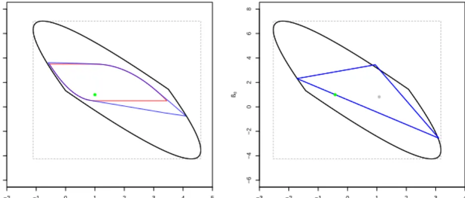
a misspecified case. The conditional Expectations are illustrated in figure 2. Figure 3 shows the corresponding identification regions. In the misspecified case the sharp marrow region is empty. Since SSR is a superset of SMR it also contains the true parameter in the correctly specified case. In the misspecified case, the parameters are meaningless in the first place, but we can compare the predictions made by the different identification regions, which are illustrated in figure 4.
21Note that the naive robustification of SCR seems to be not so easy, because one has to look at the robust estimates for ally∈[y,y] and this is not as easy as the computation of the image of [y,y] under a linear mapping.
0 1 2 3 4 5 0 5 10 15 20 25 x E(y|x) 0 1 2 3 4 5 −10 −5 0 5 10 15 20 25 x E(y|x)
Figure 2: The conditional expectationsE(Y |x) (green), E(Y|x) (blue) and E(Y|x) (red) for a well-specified (left) and a misspecified (right) situation.
−2 −1 0 1 2 3 4 5 −2 0 2 4 6 8 10 12 ß1 ß0 ● −3 −2 −1 0 1 2 3 4 −6 −4 −2 0 2 4 6 8 ß1 ß0 ● ●
Figure 3: The identification regions SMR (red), SCR (black) and SSR (blue) for a well-specified (left) and a misspecified (right) situation. The true Parameter is dotted green (for the misspecified situation the green point is the best linear predictor for y). In the misspecified case SMR is empty and the grey point indicates the unique argmin of the criterion functionQ.
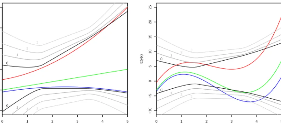
If we really want to predict the value y for a next observation with the covariate-value x we can generally only predict an interval [ˆy,y]. Here theˆ question arises, if the collection of all possible best linear predictions induced by all possibleY ∈[Y,Y] is a useful tool for this kind of prediction. Generally, the predictions are too rough and are getting rougher and rougher if we estimate
0 1 2 3 4 5 0 5 10 15 20 25 x E(y|x) 0 1 2 3 4 5 −10 −5 0 5 10 15 20 25 x E(y|x)
Figure 4: The predictions made by the regions SMR (red), SCR (black) and SSR (blue). The original conditional expectations are dashed (E(Y |x) green, E(Y|x) blue andE(Y|x) red).
and predict again and again, which is illustrated in figure 5.
0 1 2 3 4 5 0 5 10 15 20 25 x E(y|x) 0 1 2 3 0 1 2 3 0 1 2 3 4 5 −10 −5 0 5 10 15 20 25 x E(y|x) 0 1 2 3 0 1 2 3
Figure 5: Different powers (0-3) of the operator P R ◦ SCR applied to SCR((Y,Y)) for the correctly specified (left) and the misspecified (right) case: the predictions are getting rougher and rougher if we estimate and predict again and again.
Of course, if one is interested in the set of all possible best linear predictors, one can get it with SCR, but what to do with this region? If one only needs possible moments ofX, Y and XY then SCR would be helpful, but if we are
forced to make interval-valued predictions on outcomesy, we possibly use better SMR if we can rely on the linearity assumption, or SSR if we cannot do this, because it describes at least the boundsE(Y|x) andE(Y|x) better than SCR in the sense that the loss function LS is smaller or equal. One can now argue,
that SCR is, as a zonoid, a more regular or parsimonious region and therefore prefer SCR, but note that also if we restrict the problem to cases, were SMR is already a zonoid, then also in this restricted situation SCR is bigger than SMR. This is a main difference to e.g. the decision between a linear and a quadratic model: if we fit a quadratic model to a linear setting then we would get the same model as if we had chosen a linear model.
8
Concluding Remarks
We have worked out some differences between two types of identification regions in regression analysis under interval data, and discussed some of their proper-ties. Indeed, SMR, relying so-to-say on the marrow of the regression model, and SCR, taking in a collection procedure all potential combinations of data points equally seriously, can be characterized as the monotone kernel and the monotone hull of a criterion function based mapping.
Furthermore, we sketched an appealing, rigorously set-based compromise, whose properties have still to be investigated in more detail. Other topics of further research include the additional inclusion of coarse covariates and an extension to generalized linear models. For generalized linear predictors in [35] a charac-terization of the sharp collection region is already given. If also covariates are interval-valued, the description ofSCRbecomes more complicated and a refor-mulation relying on roots of likelihood-based score-functions seems promising.22
For the sharp marrow region the crucial role the conditional expectationE(Y|X) plays in the definition of SMR provides an immediate, promising link. Another direction of future research might be the analysis of models with instrumental variables. For this case a sharp characterization of SCR in terms of the sup-port function of the identified set as well as some asymptotics of corresponding estimates can be found in [4].
References
[1] Beresteanu, A., Molchanov, I., & Molinari, F. (2011): Sharp identifica-tion regions in models with convex moment predicidentifica-tions,Econometrica, 79, 1785–1821.
[2] Beresteanu, A., & Molinari, F. (2008): Asymptotic properties for a class of partially identified models, Econometrica, 76, 763–814.
22See [33], who also developed algorithms for calculating SCR’s like regions in a GLM based on an exponential model.
[3] Bolker, E.D. (1971): The zonoid problem,The American Mathematical Monthly, 78, 529–531.
[4] Bontemps, C., Magnac, T., & Maurin, E. (2012): Set identified linear Models,Econometrica, 80, 1129–1155.
[5] Bugni, F. A. (2010): Bootstrap inference in partially identified models defined by moment inequalities: Coverage of the identified set, Econo-metrica, 78, 735–753.
[6] Canay, I. A. (2010): El inference for partially identified models: Large deviations optimality and bootstrap validity,Journal of Econometrics, 156, 408–425.
[7] Cattaneo, M. E. G. V. & Wiencierz, A. (2012): Likelihood-based imprecise regression, International Journal of Approximate Reason-ing, 53, 1137–1154, extended version of the 2011 ISIPTA paper. see F. P. A. Coolen, G. de Cooman, T. Fetz, & M. Oberguggenberger (eds.):
ISIPTA ’11: Proc. Seventh Int. Symp. on Imprecise Probability: Theo-ries and Applications, 119–128, Innsbruck.
[8] ˇCern´y, M. & Rada M. (2011): On the possibilistic approach to linear regression with rounded or interval-censored data.Measurement Science Review, 11, 34–40.
[9] Chernozhukov, V., Hong, H., & Tamer, E. (2007): Estimation and con-fidence regions for parameter sets in econometric models,Econometrica, 75, 1243–1284.
[10] de Cooman, G. & Zaffalon, M. (2004): Updating beliefs with incomplete observations.Artificial Intelligence, 159, 75–125.
[11] Davey, B.A. & Priestley, H.A. (2002): Introduction to Lattices and Or-der, 2nd edition. Cambridge UP.
[12] Dempster, A.P. (1967): Upper and lower probabilities induced by a mul-tivalued mapping.Annals of Mathematical Statistics, 38, 325–339. [13] Dobra, A.& Fienberg, S. (2000): Bounds for cell entries in contingency
tables given marginal totals and decomposable graphs. Proceedings of the National Academy of Sciences of the United States of America, 97, 11885–11892.
[14] Dubois, D. (1986): Belief structure, possibility theory and decomposable confidence measures on finite sets.Computers and Artificial Intelligence, 5, 403–416.
[15] Heijmans, H.J.A.M., (1994): Morphological image operators, Academic Press, Boston.
[16] Heitjan, D. & Rubin, D. (1991): Ignorability and coarse data.The An-nals of Statistics, 19, 2244–2253.
[17] Holmes, R. N. (1975): Geometric Functional Analysis and its Applica-tions.Springer, New York.
[18] Horowitz, J. L. & Manski, C. F. (2001): Imprecise identification from incomplete data. In: G. de Cooman, T. Fine, & T. Seidenfeld (eds.):
ISIPTA’01: Proc. Second Int. Symp. on Imprecise Probabilities and Their Applications, 213–218, Maastricht, Shaker.
[19] Kwerel, S. (1983): Fr´echet Bounds, In: S. Kotz & N. Johnson (eds.):
Encyclopedia of Statistical Sciences: Volume 3, 203–209. Wiley, New York.
[20] K¨uchenhoff, H., Augustin, T. & Kunz, A. (2012): Partially identi-fied prevalence estimation under misclassification using the kappa co-efficient. International Journal of Approximate Reasoning, 53, 1168– 1182, extended version of the 2011 ISIPTA paper. see F. P. A. Coolen, G. de Cooman, T. Fetz, & M. Oberguggenberger (eds.): ISIPTA ’11: Proc. Seventh Int. Symp. on Imprecise Probability: Theories and Appli-cations, 237–246, Innsbruck.
[21] Lee, S. & Wilke, R. A. (2009): Reform of unemployment compensation in Germany: A nonparametric bounds analysis using register data,Journal of Business & Economic Statistics, 27, 193–205.
[22] Little, R. & Rubin, D. (1987): Statistical Analysis with Missing Data. Wiley, New York.
[23] Manski, C. F. (2003): Partial Identification of Probability Distributions. Springer, New York.
[24] Manski, C. F. & Molinari, F. (2010): Rounding probabilistic expecta-tions in surveys.Journal of Business & Economic Statistics, 28, 219–231. [25] Meyer, M. C. (2013): A simple new algorithm for quadratic program-ming with applications in statistics. Communications in Statistics, 42, 1126–1139.
[26] Molinari, F. (2010): Missing treatments, Journal of Business & Eco-nomic Statistics, 28, 82–95.
[27] Moon, H. R. & Schorfheide, F. (2012): Bayesian and frequentist inference in partially identified models,Econometrica, 80, 755–782.
[28] Nicoletti, C., Peracchi, F., & Foliano, F. (2011): Estimating income poverty in the presence of missing data and measurement error,Journal of Business & Economic Statistics, 29, 61–72.
[29] Nguyen, H., Kreinovich, V., Wu, B., & Xiang, G. (2011): Computing Statistics under Interval and Fuzzy Uncertainty: Applications to Com-puter Science and Engineering. Springer, Berlin/Heidelberg.
[30] P¨otter, U. (2008): Statistical Models of Incomplete Data and Their Use in Social Sciences, Ruhr-Universit¨at Bochum (Habilitation Thesis). [31] Ponomareva, M., & Tamer, E. (2011): Misspecification in moment
in-equality models: back to moment equalities?.Econometrics Journal, 14, 186-203.
[32] Rohwer, G. & P¨otter, U. (2001): Grundz¨uge der sozialwissenschaftlichen Statistik. Juventa, Weinheim.
[33] Seitz, M. (2012): Estimating partially identified parameters in gener-alized linear models under interval data (in German), Master Thesis, Department of Statistics, LMU Munich.
[34] Shafer, G. (1976): A Mathematical Theory of Evidence.Princeton U. P. [35] Stoye, J. (2007): Bounds on generalized ginear predictors with
incom-plete outcome data.Reliable Computing, 13, 293–302.
[36] Stoye, J. (2009a): Partial identification and robust treatment choice: An application to young offenders. Journal of Statistical Theory and Practice, 3, 239–254.
[37] Stoye, J. (2009b): Statistical inference for interval identified parameters. In: T. Augustin, F. Coolen, S. Moral, & M. Troffaes (eds.): ISIPTA ’09: Proc. Sixth Int. Symp. on Imprecise Probability: Theories and Applica-tions, 395–404, Durham, UK, SIPTA.
[38] Stoye, J. (2010): Partial identification of spread parameters. Quantita-tive Economics, 1, 323–357.
[39] Tamer, E. (2010): Partial identification in econometrics.Annual Review of Economics, 2, 167–195.
[40] Utkin, L. V. & Augustin, T. (2007): Decision making under imperfect measurement using the imprecise Dirichlet model.International Journal of Approximate Reasoning, 44, 322–338; extended version of the 2005 ISIPTA paper. see F. Cozman, R. Nau, & T. Seidenfeld (eds.): ISIPTA ’05: Proc. Fourth Int. Symp. on Imprecise Probabilities and Their Ap-plications, Manno.
[41] Utkin, L. V. & Coolen, F.P.A. (2011): Interval-valued regression and classification models in the framework of machine learning. In: F. P. A. Coolen, G. de Cooman, T. Fetz, & M. Oberguggenberger (eds.):
ISIPTA ’11: Proc. Seventh Int. Symp. on Imprecise Probability: Theo-ries and Applications, 371–380, Innsbruck.
[42] Vansteelandt, S., Goetghebeur, E., Kenward, M., & Molenberghs, G. (2006): Ignorance and uncertainty regions as inferential tools in a sensi-tivity analysis.Statistica Sinica, 16, 953–979.
[43] Walley, P. (1991): Statistical Reasoning with Imprecise Probabilities.
Chapman and Hall, London.
[44] Zaffalon, M. (2005): Conservative rules for predictive inference with in-complete data. In: F. Cozman, R. Nau, & T. Seidenfeld (eds.): ISIPTA ’05: Proc. Fourth Int. Symp. on Imprecise Probabilities and Their Ap-plications, 406–415, Manno.
[45] Zaffalon, M. & Miranda, E. (2009): Conservative inference rule for un-certain reasoning under incompleteness.Journal of Artificial Intelligence Research, 34, 757–821.
[46] Ziegler, G.M. (2008): Lectures on Polytopes. Graduate Texts in Mathe-matics, vol. 152, Springer, New York.
[47] Zhang, Z. (2010): Profile likelihood and incomplete data. International Statistical Review, 78, 102-116.