STATE ESTIMATION OF SPATIO-TEMPORAL PHENOMENA
A Dissertation by DAN YU
Submitted to the Office of Graduate and Professional Studies of Texas A&M University
in partial fulfillment of the requirements for the degree of DOCTOR OF PHILOSOPHY
Chair of Committee, Suman Chakravorty Committee Members, John Junkins
Sharath Girimaji Swaroop Darbha Head of Department, Rodney Bowersox
December 2016
Major Subject: Aerospace Engineering
ABSTRACT
This dissertation addresses the state estimation problem of spatio-temporal phe-nomena which can be modeled by partial differential equations (PDEs), such as pollutant dispersion in the atmosphere. After discretizing the PDE, the dynami-cal system has a large number of degrees of freedom (DOF). State estimation using Kalman Filter (KF) is computationally intractable, and hence, a reduced order model (ROM) needs to be constructed first. Moreover, the nonlinear terms, external distur-bances or unknown boundary conditions can be modeled as unknown inputs, which leads to an unknown input filtering problem. Furthermore, the performance of KF could be improved by placing sensors at feasible locations. Therefore, the sensor scheduling problem to place multiple mobile sensors is of interest.
The first part of the dissertation focuses on model reduction for large scale sys-tems with a large number of inputs/outputs. A commonly used model reduction algorithm, the balanced proper orthogonal decomposition (BPOD) algorithm, is not computationally tractable for large systems with a large number of inputs/outputs. Inspired by the BPOD and randomized algorithms, we propose a randomized proper orthogonal decomposition (RPOD) algorithm and a computationally optimal RPOD (RPOD∗) algorithm, which construct an ROM to capture the input-output behaviour of the full order model, while reducing the computational cost of BPOD by orders of magnitude. It is demonstrated that the proposed RPOD∗ algorithm could construct the ROM in real-time, and the performance of the proposed algorithms on different advection-diffusion equations.
with unknown inputs which can be treated as a wide-sense stationary process with rational power spectral density, while no other prior information needs to be known. We propose an autoregressive (AR) model based unknown input realization tech-nique which allows us to recover the input statistics from the output data by solving an appropriate least squares problem, then fit an AR model to the recovered input statistics and construct an innovations model of the unknown inputs using the eigen-system realization algorithm. The proposed algorithm outperforms the augumented two-stage Kalman Filter (ASKF) and the unbiased minimum-variance (UMV) algo-rithm are shown in several examples.
Finally, we propose a framework to place multiple mobile sensors to optimize the long-term performance of KF in the estimation of the state of a PDE. The major challenges are that placing multiple sensors is an NP-hard problem, and the optimization problem is non-convex in general. In this dissertation, first, we construct an ROM using RPOD∗ algorithm, and then reduce the feasible sensor locations into a subset using the ROM. The Information Space Receding Horizon Control (I-RHC) approach and a modified Monte Carlo Tree Search (MCTS) approach are applied to solve the sensor scheduling problem using the subset. Various applications have been provided to demonstrate the performance of the proposed approach.
DEDICATION
ACKNOWLEDGEMENTS
I am deeply indebted to many people who have helped and inspired me over the years. First and foremost, I would like to express my deepest respect and gratitude to my advisor, Prof. Suman Chakravorty for supporting and encouraging me through-out my graduate career. His positive through-outlook and enthusiasm are contagious; his keen insight would always nudge me in the right direction. Especially, I would like to thank Dr. Chakravorty for his great help and support with my career decision. This work would not have been possible without his support.
I would also like to thank my committee members, professor John Junkins, Sharath Girimaji and Darbha Swaroop for their time, encouragement and precious advice. In addition to my committee members, I would like to thank Dr. Sivakumar Rathinam for being defense examiner, and Dr. Robert Skelton for his constructive suggestions. I would like to thank Dr. Jianer Chen for his great courses. I have benefited from all of them over the years as a student or simply through friendly conversations.
I would like to thank the current and past members of Dr. Chakravorty’s group: Ali-akbar Agha-mohammadi, Saurav Agarwal, Amirhossein Tamjidi, Dilshad Raihan and Weston Faber for their friendship and for all the discussions over the years. I am especially grateful to Anshu Narang and Xiao Li Bai, for sharing their precious experience, and their persistent help. I have been fortunate to have so many friends who make my Ph.D journey enjoyable.
I would like to thank the staff in the Department of Aerospace Engineering, particularly Karen Knabe and Rose Sauser, for their constant help.
far away from home has been difficult both for me and for my parents. I would like to thank my parents for their unconditional love, and their support for every decision I have made. I also wish to thank my grandparents for their encouragement. This dissertation is dedicated to them.
TABLE OF CONTENTS
Page
ABSTRACT . . . ii
DEDICATION . . . iv
ACKNOWLEDGEMENTS . . . v
TABLE OF CONTENTS . . . vii
LIST OF FIGURES . . . x
LIST OF TABLES . . . xiii
1. INTRODUCTION . . . 1
1.1 Motivation . . . 1
1.2 Literature Review . . . 3
1.2.1 Model Reduction Methods . . . 4
1.2.2 Unknown Input Filtering . . . 8
1.2.3 Sensor Scheduling . . . 9
1.3 Contribution . . . 12
1.4 Organization . . . 13
2. RANDOMIZED PROPER ORTHOGONAL DECOMPOSITION TECH-NIQUE (RPOD) . . . 15
2.1 Introduction . . . 15
2.2 Preliminaries: POD-Galerkin Projection . . . 16
2.3 Preliminaries: Balanced Truncation and BPOD . . . 20
2.4 Simplified Analysis . . . 24
2.5 RPOD Algorithm . . . 33
2.6 Computational Results . . . 41
2.6.1 Pollutant Transport Problem . . . 41
2.6.2 Linearized Channel Flow Problem . . . 44
2.6.3 Discussion . . . 48
3. COMPUTATIONALLY OPTIMAL RANDOMIZED PROPER
ORTHOG-ONAL DECOMPOSITION (RPOD∗) . . . 52
3.1 Introduction . . . 52
3.2 Computationally Optimal Snapshot Ensemble . . . 54
3.3 RPOD∗ Algorithm . . . 57
3.4 Implementation Issues . . . 66
3.5 Comparison with Related Algorithms . . . 71
3.5.1 Comparison with BPOD . . . 71
3.5.2 Comparison with Random Projection . . . 72
3.5.3 Comparison with BPOD output projection . . . 73
3.5.4 Comparison with RPOD . . . 76
3.6 Computational Cost Analysis . . . 77
3.7 Computational Results . . . 78
3.7.1 Heat Problem . . . 79
3.7.2 Atmospheric Dispersion Problem . . . 82
3.7.3 Comparison of Computational Time . . . 86
3.8 Summary . . . 87
4. AN AUTOREGRESSIVE (AR) MODEL BASED STOCHASTIC UNKNOWN INPUT REALIZATION AND FILTERING TECHNIQUE . . . 88
4.1 Introduction . . . 88
4.2 Problem Formulation . . . 89
4.3 AR Model Based Unknown Input Realization Technique . . . 90
4.3.1 Extraction of Input Autocorrelations via a Least Squares Prob-lem . . . 90
4.3.2 Construction of the AR Based Innovations Model . . . 101
4.3.3 Extension to Estimate Unknown Input Locations . . . 106
4.4 Augmented State Kalman Filter and Model Reduction . . . 107
4.4.1 Augmented State Kalman Filter . . . 107
4.4.2 Unknown Input Estimation Using Model Reduction . . . 108
4.5 Computational Results . . . 109
4.5.1 Heat Problem . . . 110
4.5.2 Stochastically Perturbed Laminar Flow . . . 117
4.6 Summary . . . 123
5. GAUSSIAN PROCESS (GP) FOR STATE ESTIMATION . . . 125
5.1 Introduction . . . 125
5.2 Preliminaries on GP . . . 126
5.3 State Estimation Using Spatial GP Model . . . 127
5.3.2 Computational Results: 2D Heat Problem . . . 130
5.4 Summary . . . 132
6. SENSOR SCHEDULING FOR SPATIO-TEMPORAL PHENOMENA . . 135
6.1 Introduction . . . 135
6.2 Problem Formulation . . . 135
6.3 ROM Based Sensor Placement . . . 138
6.3.1 ROM and Modal Observability . . . 139
6.3.2 ROM Based Sensor Placement Optimization Problem . . . 140
6.4 ROM Based Sensor Scheduling . . . 142
6.4.1 Discussion on the Sensor Scheduling Problem . . . 143
6.4.2 Preliminaries: Information Space Receding Horizon Control (I-RHC) . . . 144
6.4.3 Preliminaries: Monte Carlo Tree Search (MCTS) . . . 148
6.4.4 Modified MCTS . . . 152
6.5 Three-Step Sensor Scheduling Framework . . . 152
6.6 Computational Results . . . 154
6.6.1 Comparison of the sensor scheduling performance using the full set and the reduced subset . . . 154
6.6.2 Sensor scheduling for 2D atmospheric dispersion problem . . . 155
6.6.3 Sensor scheduling for 3D atmospheric dispersion problem . . . 157
6.7 Summary . . . 158
7. CONCLUSION AND FUTURE WORK . . . 160
REFERENCES . . . 163
APPENDIX A. KALMAN FILTER (KF) . . . 176
APPENDIX B. EIGENSYSTEM REALIZATION ALGORITHM (ERA) . . . 178
APPENDIX C. OPTIMAL TWO-STAGE KALMAN FILTER (OTSKF) . . . 180
APPENDIX D. UNBIASED MINIMUM-VARIANCE FILTER (UMV) . . . . 182
APPENDIX E. COMPARISON OF Q-MARKOV COVARIANCE EQUIVA-LENT REALIZATION (Q-MARKOV COVER) AND ERA . . . 184
E.1 Problem Statement . . . 184
E.2 Review of the q-Markov COVER Algorithm . . . 186
E.3 Comparison with ERA . . . 189
E.3.1 Proof of Proposition 1 . . . 190
LIST OF FIGURES
FIGURE Page
1.1 State estimation procedure of spatio-temporal phenomena . . . 3 2.1 Contour plot of 2D contaminant concentration at time t = 10min,
numerical solution using full order system . . . 42 2.2 Comparison of ROM constructed using RPOD and BPOD for 2D
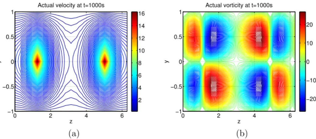
pol-lutant transport problem. (a) Comparison of extracted eigenvalues with the actual eigenvalues of the full order system. (b) Comparison of the output/state relative error over time, each plot is the average performance of 3 trials. . . 43 2.3 Contour plot of 2D linearized channel flow at t = 1000s. (a) Actual
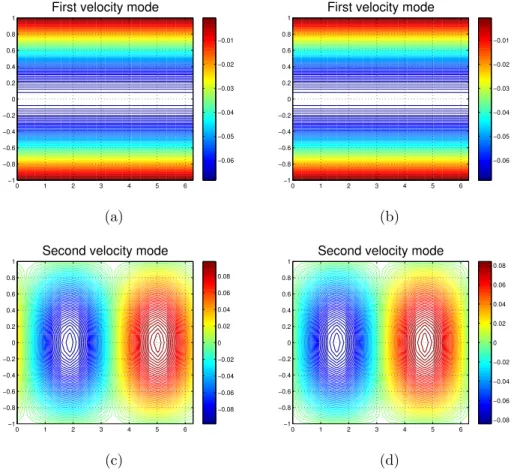
wall-normal velocity field. (b) Actual wall-normal vorticity field. . . . 45 2.4 Comparison between ROM wall-normal velocity modes and actual
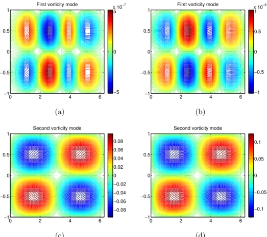
ve-locity modes. (a) Actual first veve-locity mode. (b) ROM first veve-locity mode. (c) Actual second velocity mode. (d) ROM second velocity mode. 46 2.5 Comparison between ROM wall-normal vorticity modes and actual
vorticity modes. (a) Actual first vorticity mode. (b) ROM first vor-ticity mode. (c) Actual second vorticity mode. (d) ROM second vorticity mode. . . 47 2.6 Comparison of eigenvalues extract by RPOD and BPOD for linearized
channel flow problem . . . 48 2.7 Comparison of ROM errors between RPOD and BPOD for linearized
channel flow problem. (a) Comparison of the output relative error over time. (b) Comparison of the state relative error over time. Each plot is the average performance of 20 trials. . . 49 2.8 Simulation results using RPOD for linearized channel flow problem
when BPOD is not feasible. (a) Eigenvalues extracted using RPOD. (b) Output relative errors using RPOD. . . 50
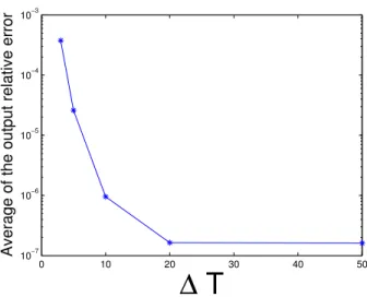
3.1 This figure explains when to take the snapshots in RPOD∗. The snap-shots are taken at every ∆T time, and the averaged output relative error is plotted as a function of ∆T. . . 67 3.2 Comparison of time domain errors between RPOD∗, BPOD and BPOD
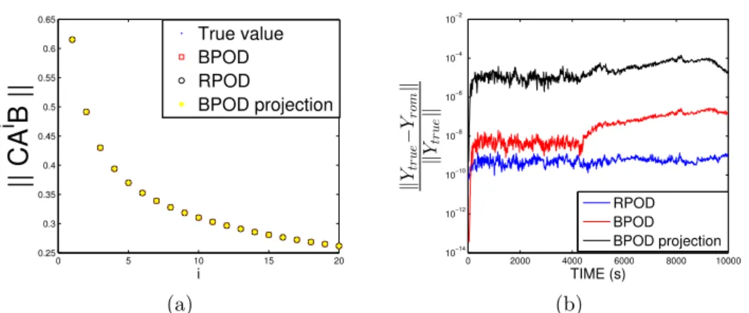
output projection for heat transfer problem. (a) Comparison of Markov parameters. (b) Comparison of output relative errors. . . 81 3.3 Comparison of frequency responses between RPOD∗, BPOD and BPOD
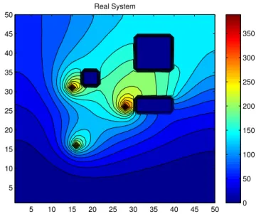
output projection for heat transfer problem. (a) Comparison of fre-quency responses. (b) Comparison of frefre-quency response errors. . . . 82 3.4 Contour plot of air pollutant concentration att = 200s. . . 84 3.5 Comparison of time domain errors between RPOD∗and BPOD output
projection for atmospheric dispersion problem. (a) Comparison of Markov parameters. (b) Comparison of output relative errors. . . 85 3.6 Comparison of frequency responses between RPOD∗ and BPOD
out-put projection for atmospheric dispersion problem. (a) Comparison of frequency responses. (b) Comparison of frequency response errors. 86 4.1 Comparison of the recovered input autocorrelations with actual
un-known input autocorrelations for heat problem. . . 112 4.2 Comparison of input autocorrelation relative error using full order
model with ROM for heat problem. . . 113 4.3 Unknown input filtering for heat problem using ROM. State
estima-tion error and 3σ bounds for two randomly chosen states. . . 114 4.4 Comparison of the performances of AR model based algorithm with
OTSKF and UMV algorithms for heat transfer problem. The ARMSE is plotted as a function of NSR. . . 116 4.5 Comparison of recovered input autocorrelations with actual unknown
input autocorrelations for stochastically perturbed laminar flow. . . . 120 4.6 Comparison of input autocorrelation relative error using full order
model and ROM for stochastically perturbed laminar flow. . . 121 4.7 Unknown input filtering for stochastically perturbed laminar flow
us-ing ROM. State estimation errors and 3σ bounds for two randomly chosen states. . . 122
5.1 GP model learned from training data at timet0 for 1D heat problem. 129
5.2 Comparison of state estimation at t ≥ t0 using GP model and ROM
for 1D heat problem. (a) Comparison of state estimation error and 3σ bounds. (b) Comparison of normalized RMSE. . . 131 5.3 GP model learned from training data at t0 for 2D heat problem. (a)
Training Data (b) GP model. . . 132 5.4 Comparison of state estimation at t ≥ t0 using GP model and ROM
for 2D heat problem. (a) Comparison of state estimation error and 3σ bounds. (b) Comparison of normalized RMSE. . . 133 6.1 This figure illustrates the differences between constructing subset
sen-sor locations S∗ using local maxima criterion and threshold . . . 142 6.2 Outline of MCTS approach [1] . . . 149 6.3 Parallelization approaches for MCTS [2] . . . 151 6.4 Comparison of optimal reward using S∗ and S for 1D heat problem.
The optimal reward usingS∗ is plotted as a function of design param-eters nl and δ. . . 156
6.5 Comparison of I-RHC, modified MCTS, exhaustive search and myopic approaches for 2D atmospheric dispersion problem. . . 157 6.6 State estimation using I-RHC, modified MCTS and myopic approaches.158 6.7 Comparison of I-RHC and myopic approaches for 3D atmospheric
LIST OF TABLES
TABLE Page
2.1 Comparison of performance (BPOD V.S. RPOD) . . . 49 3.1 Computational Complexity Analysis for RPOD∗ and BPOD Output
Projection . . . 77 3.2 Parameters of Heat and Atmospheric Dispersion System . . . 80 3.3 Comparison of Computational Time using RPOD∗ and BPOD output
projection for Heat Transfer and Atmospheric Dispersion . . . 87 4.1 Performances of the AR model based algorithm, OTSKF and UMV
for Heat Problem . . . 116 4.2 Performances of the AR model based algorithm, UMV and OTSKF
1. INTRODUCTION
1.1 Motivation
Many real-world phenomena can be viewed as spatio-temporal processes which are modeled by partial differential equations (PDEs). For example, the motion of fluids such as precipitation [3], ocean currents [4, 5], air pollution [6] and water flow in a pipe [7] can be described by Navier-Stokes Equations [8]. In addition, the temperature distribution of a large battery pack [9], biological phenomena [10] , power system state-time behavior [11] and many other engineering applications are also modeled by PDEs.
Historically, there has been a lot of theoretical research in the Control Systems community on the estimation and control of systems driven by PDEs [8, 12–15]. A standard approach is to transform PDEs to a set of ordinary differential equations (ODEs) by discretizing the PDEs in space using the finite difference method (FDM) or finite element method (FEM). The discretized system has a large number of de-grees of freedom (DOF) which leads to the following problem: state estimation of such a system using standard Kalman Filter (KF) is not computationally tractable. Therefore, a reduced order model (ROM) constructed via model reduction algorithms is used for state estimation. The benefit of using an ROM based KF is that the ex-pensive computations for constructing the ROM can be done offline, and the online state estimation computations are essentially trivial.
In addition, in order to estimate the states of stochastic dynamical system, it is generally assumed that all system parameters, noise covariance, and inputs are known. However, in practice, unknown inputs are often present in the systems due to the unmodeled dynamics, nonlinear terms or external disturbances. The state
estimation of stochastic systems in presence of unknown inputs is known as the unknown input filtering (UIF) problem, and has been investigated for decades.
There are many applications where the unknown inputs can be modeled as a stochastic process. In [16], a stochastic disturbance model is used to force the lin-earized Navier-Stokes equation, which leads to a simulated flow state with certain second-order statistics closely matching the flow statistics computed from the Di-rect Numerical Simulation (DNS) of turbulent channel flow. Based on this result, the state estimation of perturbed laminar flows is considered in [17]. It shows that the external disturbances and nonlinear coupling terms can be modeled as unknown stochastic inputs, which perturb the linearized Navier-Stoke equations. Thus, the state estimation problem of such system is transformed into the unknown input fil-tering problem with stochastic unknown inputs. Also, there is some research that considers Kalman filtering with unknown noise covariances. The process noise is as-sumed to be white noise with unknown covariance [18, 19], while in our research, the process noise can be colored in time as well. There are also applications of unknown stochastic inputs estimation in signal processing, such as the wideband power spec-trum estimation [20], where the problem is to recover the unknown power specspec-trum of a wide-sense stationary signal from the obtained sub-Nyquist rate samples. In this dissertation, we consider the UIF problem when the unknown inputs can be modeled as stochastic processes.
Another important problem considered in this dissertation is to place multiple mobile sensors to optimize the long-term behavior of the KF in the estimation of the state of a PDE. Since sensors have become much smaller and less expensive in the last few decades, there is increasing attention of using mobile sensors for moni-toring spatio-temporal phenomena. Moreover, installing and maintaining stationary sensors are costly, and in scenarios when the phenomena changes in a short
dura-tion, stationary sensors collect limited information. The major challenges are that placing multiple sensors is an NP-hard problem [21], and the optimization problem is non-convex in general. Hence, most algorithms focus on placing sensors which can optimize performance of the current time instant, i.e., a myopic policy.
In this context, the motivation for this research arises from the desire to design a KF based approach for estimating and predicting spatio-temporal phenomena. The proposed approach is capable of handling uncertainties as well as unknown inputs. The performance of the state estimator is optimized by placing multiple mobile sensors to take measurements, and most importantly, the approach can be implemented efficiently. The general structure of the proposed approach is shown in Fig. 1.1.
Spatio-Temporal Dynamical System Model Reduction
Unknown Input Realization Sensor Scheduling State Estimation
Figure 1.1: State estimation procedure of spatio-temporal phenomena
1.2 Literature Review
In this section, we review the literature most relevant to our research. Section 1.2.1 reviews different model reduction techniques that have been widely used. In Section 1.2.2, we give an overview of the unknown input filtering methods, and in Section 1.2.3, we review the literature relates to the sensor placement problem. The open research problems are enumerated in each subsection respectively.
1.2.1 Model Reduction Methods
Model reduction has attracted considerable attention in the past several decades. It is a technique that constructs a lower-dimensional subspace to approximate the original high-dimensional dynamic system.
The Proper Orthogonal Decomposition (POD), also known as Karhunen-Loeve decomposition or principle component analysis, followed by a Galerkin projection has been used extensively in the Fluids community to produce reduced order models (ROMs) of fluid phenomena such as turbulence and fluid structure interaction [22– 24]. A review of the POD is given in [25]. An empirical basis of orthonormal eigenfunctions is obtained from experimental or simulation data, and the original higher-dimensional system is projected onto this basis. The POD modes are optimal in the sense that the energy captured in the ROM are optimized, and the most significant modes are the ones that carry most of the kinetic energy. However, the most energetic modes are not always the most dynamically significant ones. Hence, a major disadvantage of POD technique is that the ROM constructed using POD is not accurate [26]. Techniques to improve performance of POD are reviewed in [27].
In the context of control theory, balanced truncation introduced in [28] has been successfully applied to linear dynamical systems. Balanced truncation yields a stable reduced system with a bounded approximation error. Both the inputs and outputs of the dynamical system are taken into account, and consequently, the ROM captures the input-output behavior of the original system. However, balanced truncation suffers from high computational complexity when generating the controllability and observability Gramians for large scale systems.
To reduce the computational cost of balanced truncation, Balanced POD (BPOD) [29, 30], which is based on the snapshot POD and balanced truncation has been
proposed. Balancing transformations are constructed using the impulse responses of both the primal and adjoint system, and hence, the most controllable and observable modes can be kept in the ROM. In 1978, Kung [31] presented a new model reduction algorithm in conjunction with the singular value decomposition (SVD) technique, and the eigensystem realization algorithm (ERA) [32] was developed based on this technique. The BPOD is equivalent to the ERA procedure [33], and forms the Hankel matrix using the primal and adjoint system simulations as opposed to the input-output data as in ERA. More recently, there has been work on obtaining information regarding the dominant modes of the system based on the snapshot POD, followed by an eigendecomposition of an approximating linear operator, called the dynamic mode decomposition (DMD) [34, 35].
The primary drawback of BPOD and ERA is that for a large scale system, such as that obtained by discretizing a PDE, with a large number of inputs/outputs, the computational burden incurred is very high. There are two main parts to the computation: First is to collect datasets from computationally expensive primal and adjoint simulation in order to generate the Hankel matrix. The second part is to solve the SVD problem for the resulting Hankel matrix.
Improved algorithms have been proposed to reduce the computational complexity of BPOD. For example, [30] proposed an output projection method to address the problem when the number of outputs is large. The outputs are projected onto a small subspace via an orthogonal projection Ps that minimizes the error between the full
impulse response and the projected impulse response. However, the method cannot make any claim regarding the closeness of the solution to one that is obtained from the full Hankel matrix, and is still faced with a very high computational burden when both the numbers of inputs and outputs are large. There have also been methods proposed [36] to reduce the number of snapshots. First, the DMD is used to estimate
the slowly decaying modes that dominate the long-term behavior of the impulse responses, and then analytic expressions are formulated for the contribution of these modes. Therefore, there is no need to run the long impulse response simulations. However, the primary problem regarding large number of inputs/outputs remains the same.
Randomized algorithms motivated by problems in large-scale data analysis have been developed recently. The advantage of the randomized algorithm is that: 1) often the execution time or space requirement of a randomized algorithm is smaller than that of the best deterministic algorithm, and 2) it lead to a simpler algorithm to implement. There are two major classes of randomization algorithms used for low-rank matrix approximations and factorizations: random sampling algorithms [37] and random projection algorithms [38, 39].
For a large scale matrix H, random sampling algorithms construct a rank k approximation matrix ˆH by choosing and rescaling some columns ofH according to certain sampling probabilities [38], so the error satisfieskH−Hkˆ F ≤ kH−H(k)kF+
kHkF, with high probability, where H(k) is a best rank k approximation of H,
is a specified tolerance, and kHkF denotes the Frobenius norm of H. The improved
algorithm proposed in [39] is to sample some columns according to leverage scores, where the leverage scores are calculated by performing the SVD of H, so that the error satisfies kH−Hkˆ F ≤(1 +)kH−H(k)kF,with high probability.
A recently developed “Scenario Method” for systems and control design [40, 41] can also be related to the random sampling algorithm. For a robust convex opti-mization problem, the number of optiopti-mization variable d is finite, while the num-ber of constraints may be infinite. The scenario method randomly samples Ns
convex constraints from the uncountable set of constraints, and with the bound Ns ≥ 2(log(β1) +d), the optimal solution can be guaranteed to satisfy an - fraction
of the constraints, with probability no smaller than 1−β, where and β are design parameters.
In random projection method [37], the large matrix H is projected on to an orthonormal basis Q such that the error satisfies kH−QQ∗Hk ≤(1 +)kH−H(k)k
with high probability, where kHk denotes the spectral 2-norm of H, x∗ denotes the complex conjugate transpose of x. A Gaussian test matrix Ω is generated, and the orthonormal basis Q is constructed by performing a QR factorization of the matrix product HΩ.
A direct application of both the random sampling algorithm and random projec-tion algorithm would require the full Hankel matrix to be constructed, however, such a construction of the Hankel matrix is computationally prohibitive when the num-ber of inputs/outputs is large. Further, in random sampling algorithm, the leverage scores are calculated by performing the SVD of the Hankel matrix, which is also computationally prohibitive owing to the size of the problem.
In this dissertation, we aim to reduce the computational costs and storage re-quirements of BPOD while keeping the same accuracy as BPOD. In Section 2, we propose a Randomized POD (RPOD) algorithm, which is closely related to the “Sce-nario Method”. We randomly choose a subset of the input/output trajectories and construct a sub-Hankel matrix, which has the same rank as the full Hankel matrix with a high probability. We derive a bound on the number of input/output trajecto-ries to be sampled, and the derivation of our bound, albeit different from the bound in [40], is nonetheless inspired by the developments in that reference. Similar to the BPOD algorithm, the controllable and observable modes are retained in the ROM, the Markov parameters of the ROM are close to the Markov parameters of the full order system, while the error is bounded. The computations required by RPOD are orders of magnitude cheaper when compared to the BPOD/BPOD output projection
algorithm.
In Section 3, we propose a computationally optimal RPOD (RPOD∗) algorithm, which is closely related to the random projection algorithm. The RPOD∗ algorithm can be viewed as applying the random projection on the full Hankel matrix H twice without constructing the full Hankel matrix H. We believe that RPOD∗ is the most computational efficient POD algorithm.
1.2.2 Unknown Input Filtering
Observers are dynamic systems that can be used to estimate the state of a plant using its input-output measurements. In some cases, the inputs to the plant are un-known or partially un-known, which leads to the development of the so-called unun-known input observer (UIO). The unknown input observer has been well established for de-terministic systems [42–44]. Various methods of building full-order or reduced-order observers have been developed, such as [45–47]. Recently, sliding mode observers have been proposed for systems with unknown inputs [48]. The design parameters and matrices need to be well chosen to satisfy certain conditions in order for the observers to perform well. For systems without the “observer matching” condition being satisfied, a high-gain approach is proposed [49]. The high-gain observers are used as approximate differentiators to obtain the estimates of the auxiliary outputs. In the presence of measurement noise, the high-gain observer amplifies the noise, and extra care needs to be taken when designing the gain matrix.
For stochastic systems, the state estimation problem with unknown inputs is known as unknown input filtering (UIF) problem, and many UIF approaches are based on the Kalman filter [50–52]. When the dynamics of the unknown inputs is available, for example, if it can be assumed to be a wide-sense stationary (WSS) pro-cess with known mean and covariance, one common approach called Augmented State
Kalman Filter (ASKF) is used, where the states are augmented with the unknown inputs [53]. To reduce the computational complexity of ASKF, optimal two-stage Kalman filters (OTSKF) and optimal three-stage Kalman filters have been developed to decouple the augmented filter into two parallel reduced-order filters by applying a U-V transformation [54–56]. When no prior information about the unknown input is available, the invalid assumption about the model may have a major adverse effect on the filter’s performance, and hence, an unbiased minimum-variance (UMV) filter-ing technique has been developed [57, 58]. The problem is transformed into findfilter-ing a gain matrix such that the trace of the estimation error matrix is minimized. The “observer matching” condition needs to be satisfied, and certain algebraic constraints must be satisfied for the unbiased estimator to exist. When the assumed unknown input model used in OTSKF is accurate, the performance of OTSKF is better than UMV algorithm in the sense that the error covariances are smaller, otherwise, UMV algorithm is more accurate than OTSKF.
In Section 4 we propose a new UIF algorithm when the unknown inputs can be treated as a wide-sense stationary process with rational power spectral density, while no other prior information needs to be known. The algorithm is based on the system identification technique, which is more accurate than OTSKF and UMV algorithms, and can tolerate more sensor noise. A milder assumption than the “observer match-ing” condition needs to be satisfied. Also, the algorithm we propose can be applied to estimate the locations of the unknown inputs.
1.2.3 Sensor Scheduling
The optimal sensor placement problem is to place multiple sensors in a spatial field, which can maximize a performance metric. Optimal sensor placement in spatial field faces the challenges such as placing multiple sensors is NP-hard [21], and the
optimization problem is non-convex in general. As the number of sensors or the num-ber of possible sensor locations increases, an exhaustive search for global optimum is computationally infeasible, so many near-optimal or sub-optimal sensor placement methods have been developed. For the purpose of field estimation, there are two major classes of sensor placement techniques: Gaussian Process (GP) based [59, 60] and mode shape based algorithms [61, 62].
The Gaussian Process (GP) [63] has been widely used to estimate and predict spatial phenomena. For example, in [59], the temperature measurements in two-dimensional space are assumed to be spatially correlated, and can be modeled by a GP. Given measurements at some locations, we can predict the temperature at arbi-trary locations. A near-optimal sensor placement approach is developed by adding sensors in sequence, and choosing the next sensor which provides the maximum in-crease in mutual information. However, for the spatio-temporal phenomena which also evolve with time, predictions using the learned GP model could result in large errors. Hence, current research has focused on modelling the desired phenomena using a spatio-temporal GP, with a mobile sensor network [64–66]. However, in such a case, a more complicated GP model needs to be learned, and the computational complexity of GP regression increases as the number of observations increases.
When the spatio-temporal phenomena can be modeled by PDEs, one research direction focuses on placing the sensors using spatial structure of the underlying phenomena [61, 62]. For example, in [67], sensors are placed using the eigenfunctions of the PDEs and is formulated as an optimization problem to maximize the system observability. In [68–70], the original systems are projected onto lower-dimensional subspace using the POD algorithm. The sensors are placed at the extrema of the POD projection bases, and the ROMs are used for state estimation, which is com-putationally tractable.
The mobile sensor placement problem can be viewed as an extension of the static sensor placement problem, which allows the sensors to move in time. When the sensors are placed to maximize the performance metric at the next time instant, it results in a myopic sensor scheduling problem. The non-myopic sensor scheduling problem is to optimize the performance metric over a suitably long time-horizon. Myopic scheduling is attractive due to its low computational complexity and ease of implementation, while the use of non-myopic scheduling is imperative for dynami-cal systems as it can perform significantly better than myopic scheduling. This is because myopic decisions do not take into account the long-term effects of these decisions. Although the sensor scheduling problem has been well studied, applying the non-myopic algorithms on large scale spatio-temporal system is still not com-putationally tractable. Hence, most mobile sensor placement algorithms are myopic when monitoring spatio-temporal systems.
There are two major classes of non-myopic sensor scheduling algorithms. The first class is based on the exhaustive tree search [71, 72], which requires the enumeration at every iteration. The benefits of the branch-and-bound based tree search algorithm is its wide range of applications, while the size of the decision space poses challenge. Another class of sensor scheduling algorithm is to relax the non-convex optimization problem into a convex problem [73,74]. The advantage of using the convex relaxation algorithm is that once the problem is convex, it can be solved efficiently.
In Section 6, we apply two non-myopic sensor scheduling algorithms to place multiple mobile sensors for spatio-temporal systems and compare the performance with myopic algorithm.
1.3 Contribution
This dissertation focuses on monitoring and predicting spatio-temporal phenom-ena which can be modeled by partial differential equations (PDEs), such as pollutant dispersion. Three problems are solved in this dissertation. First, new model reduc-tion algorithms are proposed to reduce the computareduc-tional cost of state estimareduc-tion using the Kalman Filter (KF). Next, we consider the problem of state estimation in the presence of unknown inputs, and provide a new unknown input realization algorithm. Finally, we present a framework for non-myopic sensor scheduling to op-timize the performance of a KF monitoring a spatio-temporal process. The major contributions are as follows:
• Model Reduction: We present a new perspective to analyze the relation between the snapshot ensembles and ROM. The concept of computationally optimal snapshot ensembles is introduced, and we propose a RPOD∗ algorithm which can reduce the computational cost of BPOD by orders of magnitude, while keeping the same accuracy. We also relate the RPOD∗ algorithm to randomized algorithms.
• Unknown Input Realization: We propose an autoregressive (AR) model based unknown input realization technique, which constructs an unknown input model using only the output information. The unknown inputs are assumed to be a wide-sense stationary process with rational power spectral density while no other information needs to be known. The so-called matching condition is avoided, and sufficient conditions for the convergence of estimation error in the presence of unknown inputs are derived. The ROM constructed using RPOD∗ algorithm is used to reduce the computational complexity. We show that the performance of AR model based algorithm is significantly better than
the OTSKF and UMV algorithms (two other UIF algorithms).
• Sensor Scheduling: We propose a three-step framework to place multiple mobile sensors for spatio-temporal systems efficiently. First, an ROM is con-structed using RPOD∗algorithm, and an optimization problem using the ROM is formulated to reduce the possible locations of sensors into a subset. Two sensor scheduling algorithms are used to place mobile sensors in a receding horizon fashion. The proposed algorithm is tested on moderate to large scale spatio-temporal phenomena.
This research has been reported in several publications. Different POD based model reduction algorithms are reported in [75–78]. The AR model based unknown input realization method is reported in [79, 80].
1.4 Organization The rest of the dissertation is organized as follows:
Section 2presents a brief review of existing model reduction techniques which are related to our research, with a simplified analysis of BPOD in a new perspective. The ROM is related to the controllable and observable eigenmodes of the dynamical system, which reveals some fundamental insights into the model reduction technique. A new model reduction algorithm RPOD is presented which can reduce the com-putational cost required by existing approaches, and several comcom-putational results comparing RPOD with BPOD are provided.
Section 3extends the study of Section 2, and proposes a computationally opti-mal RPOD algorithm, which can further reduce the computational cost of RPOD. Discussion of implementation issues and comparison with all related model reduction algorithms are included. The computational complexity analysis is provided, and the proposed algorithm is tested on several advection-diffusion problems.
Section 4 considers the design of a stochastic unknown input realization algo-rithm. The problem is formulated, and necessary conditions for convergence of the estimation error are analyzed. Applications on heat problem and linearized channel flow problem are presented to demonstrate the performance of the proposed algo-rithm.
Section 5discusses state estimation of spatio-temporal phenomena using Gaus-sian Process (GP) model. GPs are briefly reviewed, and simulation results are shown to illustrate the issues with using GP for estimation of spatio-temporal phenomena. Section 6proposes a three-step sensor scheduling framework for large scale sys-tems. First, an ROM is constructed using RPOD∗ algorithm. Then the possible locations are reduced onto a subset using the ROM. Two sensor scheduling ap-proaches are applied to place multiple mobile sensors in a receding horizon control fashion. Computational results are presented to compare performances of different sensor scheduling approaches.
2. RANDOMIZED PROPER ORTHOGONAL DECOMPOSITION TECHNIQUE (RPOD)
2.1 Introduction
The main goal and contribution of this dissertation is to develop a model reduc-tion algorithm for large scale systems with a large number of inputs/outputs. As discussed in Section 1, the spatio-temporal phenomena we are interested in can be modeled by partial differential equations (PDEs), and after discretizing the PDEs using finite element or finite difference method, the system can have dimension of O(105∼9). Standard state estimation and control design methods for such a system
are computationally intractable, and hence, the use of a reduced order model (ROM) is necessary.
In this section, we begin by reviewing standard model reduction methods which are related to our work. Proper orthogonal decomposition (POD) with Galerkin projection is a standard model reduction approach, where the original system is pro-jected onto a lower-dimensional subspace using a set of orthogonal bases. In linear control theory, balance truncation is a widely used model reduction approach, which takes into account of both the inputs and outputs, and hence, the ROM can cap-ture the input-output behavior of the original system. Balanced proper orthogonal decomposition (BPOD) algorithm is based on the snapshot POD and balance trun-cation, and is most related to our work. The goal of this section is to propose a randomized proper orthogonal decomposition (RPOD) algorithm, which reduce the computational cost of BPOD while the ROM retaining almost the same information as BPOD, especially for the system with a large number of inputs/outputs.
the main idea of POD via Galerkin projection. In Section 2.3, we introduce the balance truncation approaches, with a detail description of BPOD algorithm. Then we analyze the BPOD algorithm in a simplified fashion in Section 2.4. The simplified analysis is crucial to understanding the fundamental of the RPOD algorithm. We propose the RPOD algorithm in Section 2.5, and we show that the sub-Hankel matrix we construct retains almost the same information as the full Hankel matrix in terms of the numbers and accuracy of the underlying modes. In Section 2.6, we compare the simulation results using RPOD and BPOD for several advection-diffusion equations.
2.2 Preliminaries: POD-Galerkin Projection
POD-Galerkin Projection is a projection method where the dynamical system is projected onto a subspace of the original space. POD provides a method for finding the best approximating subspace to a given set of data in an optimal least-square sense, and Galerkin projection is a standard technique to reduce partial differential equations with a method of lines to a system of ordinary differential equations. POD Algorithm. Consider a high-dimensional Hilbert space H=<N, whereN is
large, and a given set of data in H:
X ={x1(t), x2(t),· · · , xm(t)} ∈ <N×m, (2.1)
where t ∈[0, T]. POD method [81] aims to find an orthogonal projectionPs :H →
Hd which projects the original data onto a d-dimensional subspace that minimizes
the total least-squares distances:
kX−PsXk2 = m X i=1 Z T 0 kxi(t)−Psxi(t)k2dt, (2.2)
Solving the optimization problem (2.2) leads to an eigenvalue problem:
Kφi =λiφi, i= 1,· · · , N, (2.3)
where K ∈ <N×N is called the kernel and is defined as:
K = m X i=1 Z T 0 xi(t)xi(t)0dt, (2.4)
where (.)0 denotes the transpose of (.).
By definition,K is a symmetric positive semi-definite matrix with real, nonneg-ative ordered eigenvalues λ1 ≥ λ2 ≥ · · · ≥ λN ≥ 0. The optimal subspace Hd of
dimensiondis given by Hd= span {φ1,· · · , φd}, and the eigenvectorsφi, i= 1,· · ·d
are called the POD modes. The major results of POD is given as follows [82]. Theorem 1 Let K be the kernel of the data, and λ1,· · · , λN ≥ 0 be the ordered
eigenvalues of K. Then it holds
min Hd kX−PsXk= N X i=N−d+1 λi, (2.5)
where the minimum is taken over all subspaces Hd of dimension d. Further, the
optimal orthogonal projection Ps :H → Hd, with PsPs0 =I is given by:
Ps= d X
i=1
φiφ0i. (2.6)
For a large scale system, solving eigenvalue problem for matrixK ∈ <N×N, where
N = O(105 ∼ 109) is computationally intractable. Therefore, in [83], the method of snapshots is introduced to approximate the kernel matrix K without explicitly calculating (2.4). Snapshots are constructed from the trajectories of the dynamical
system by evaluating them at certain discrete time instances t1,· · ·tm ∈ [0, T], and
the kernel matrix is approximated by:
K =
m X
i=1
x(ti)x(ti)0. (2.7)
where x(ti) is the instantaneous system state at time ti, and m n is the number
of snapshots. Denote the snapshot ensemble as X =
x(t1),· · · , x(tm)
∈ <N×m.
In the method of snapshots, instead of solving eigenvalue problem for K = XX0 ∈ <N×N, one considers to solve an m×m eigenvalue problem:
X0Xvj =λjvj, j = 1,· · ·, m, (2.8)
where λ1 ≥ · · · ≥ λm are the ordered eigenvalues, and vj are the corresponding
eigenvectors. The POD modes are given by:
φj =
1
p
λj
Xvj, j = 1,· · · , d. (2.9)
After constructing POD modes Φ ={φ1,· · · , φd}, the ROM is obtained by
pro-jecting dynamical system onto the POD modes via Galerkin projection.
Galerkin Projection. Consider a dynamical system which is governed by PDE with variable x(t) ∈ H. If the spatial domain is Ω, then H is a space of functions defined on Ω. The dynamical system satisfies
˙
x(t) = f(x(t)), (2.10)
wheref :H → His a spatial differential operator. Given a subspace Hd⊂ H, which
evolves on Hd and approximates the original dynamical system. The ROM is given
by:
˙
xd(t) = Psf(xd(t)), (2.11)
where Ps :H → Hd is the orthogonal projection map, and xd(t)∈ Hd.
Letφk ∈ H, k= 1,· · ·dbe an orthogonal basis for the subspace, thenxd(t) could
be represented by xd(t) = d X k=1 ak(t)φk, (2.12)
whereφkare time-independent basis functions, and ak(t) are the corresponding time
coefficients. Therefore, the ROM can be obtained using POD modes, and the evolu-tion of the time coefficients are governed byr ordinary differential equations (ODEs) as follows ˙ ak(t) =φ0kf(xd(t)) =φ0kf( d X j=1 aj(t)φj), k = 1,· · ·d. (2.13)
Discussion. The advantages of using POD approach are summarized as follows. First, the POD modes are constructed from the sampled data, and hence, the ap-proach can be applied to linear and nonlinear system, as well as to parametrically varying systems. Also, solving eigenvalue problem takes time O(m3), where m is
the number of snapshots, and m N. However, POD modes are sensitive to the snapshot ensemble X, and could only capture the system behavior for a particular time range for particular inputs. A good snapshot set selection leads to a better performance of ROM, while there is no guidance on how to select the snapshots.
Furthermore, POD approach only takes into account the system inputs, and hence, inefficient modes may be obtained. From the control point of view, the input-output relationship is important, and needs to be taken into consideration.
2.3 Preliminaries: Balanced Truncation and BPOD
Balanced Truncation. Balanced truncation is a standard model reduction algorithm which is introduced by [84]. Both the inputs and outputs are taken into account, and hence, the ROM can capture the input-output behavior of the original dynamical system.
For a linear time-invariant (LTI) stable discrete-time input-output system:
xk+1 =Axk+Buk,
yk=Cxk, (2.14)
where xk ∈ <N, uk ∈ <p, andyk ∈ <q is the state vector, input vector, and output
vector at time tk respectively.
The adjoint/dual system is defined as:
zk+1 =A0zk+C0vk,
ˆ
yk =B0zk, (2.15)
where zk is the adjoint state vector at timetk.
Balanced truncation aims to find a transformation matrixTs, such that the
con-trollability and observability Gramians
Wc= ∞ X k=0 AkBB0(A0)k, Wo= ∞ X k=0 (A0)kC0CAk (2.16)
are equal and diagonal.
The transformation matrixTs is constructed by solving the eigenvalue problem:
Wcoφj =λjφj, j = 1,· · ·n, (2.17) where Wco = WcWo, λ1 ≥ · · · ≥ λn, and Ts = φ1,· · · , φr ∈ <n×r contains the first r eigenmodes.
The ROM is given by:
ak+1 =Ts−1ATsak+Ts−1Buk,
ykr =CTsak. (2.18)
And the controllability and observability Gramians of the ROM are:
˜
Wc= ˜Wo = Σ, (2.19)
where Σ is a diagonal matrix, with elementσi, i= 1,· · · , r, andσi =
√
λi are known
as the Hankel singular values of the system.
Balanced truncation has the following property. Theorem 2 The error bound on the output is:
kyk−yrkk ≤2 n X
i=r+1
σikukk. (2.20)
Same as POD approach, generating the controllability and observability Grami-ans for large scale system is computationally expensive, and hence, in [29, 30], bal-anced truncation using the method of snapshots are proposed which do not require to compute the Gramians, and BPOD algorithm proposed in [30] is reviewed here.
BPOD Algorithm. BPOD algorithm constructs the snapshot ensemblesXb, Zb
by perturbing the primal system (2.14) and adjoint system (2.15) with impulse re-spectively, and it is shown in [85] that the Gramians in (2.16) can be approximated as
Wc≈XbXb0, Wo ≈ZbZb0. (2.21)
BPOD constructs two bi-orthogonal transformation matricesTb, Sbby solving the
singular value decomposition (SVD) problem of
Hb =Zb0Xb, (2.22)
where Hb is known as Hankel matrix.
The BPOD algorithm is summarized in Algorithm 1.
Discussion. Recall the impulse response snapshot ensembles collected in the BPOD are: Xb = [x1(t1),· · · , xp(t1),· · · , x1(tm),· · · , xp(tm)] | {z } N×pm , Zb = [z1(ˆt1),· · · , zq(ˆt1),· · · , z1(ˆtn),· · · , zq(ˆtn)] | {z } N×qn , (2.29)
and the Hankel matrix is:
Hb =Zb0Xb ∈ <qn×pm. (2.30)
There are two main parts to the computation:
Algorithm 1 BPOD Algorithm
1. Collect impulse response Xb of the primal system (2.14):
Use bi, i = 1,· · · , p as initial conditions for (2.14) with uk = 0. Take m
snapshots at discrete times t1, t2,· · · , tm, and
Xb = [x1(t1),· · · , xp(t1),· · · , x1(tm),· · ·, xp(tm)], (2.23)
where xi(tk) is the state snapshot at time tk with bi as the initial condition,
k = 1,2,· · · , m and i= 1,2,· · · , p.
2. Collect impulse response Zb of the adjoint system (2.15):
Use c0j, j = 1,· · · , q as initial conditions for (2.15) with vk = 0. Take n
snap-shots at time step ˆt1,ˆt2,· · · ,ˆtn, and
Zb = [z1(ˆt1),· · · , zq(ˆt1),· · · , z1(ˆtn),· · · , zq(ˆtn)], (2.24)
where zj(ˆtk) is the state snapshot of the adjoint system at time ˆtk with c0j as
the initial condition, k = 1,2,· · · , n and j = 1,2,· · · , q. 3. Construct Hankel matrixHb:
Hb =Zb0Xb, (2.25)
4. Solve the SVD problem of Hb:
Hb = Lb L1 Σb 0 0 Σ1 R0b R01 , (2.26)
where Σb contains the firstl non-zero singular values, and (Lb, Rb) are the
cor-responding left and right singular vectors. Σ1 contains the rest of the singular
values.
5. Construct the BPOD bases:
Tb =XbRbΣ −1/2 b , Sb = Σ −1/2 b L 0 bZ 0 b. (2.27)
6. The ROM is:
Ab =SbATb,
Bb =SbB,
hence, the construction of Hb takes time O(pqmnN).
2. The computational cost to solve the SVD ofHb is O(min{p2m2qn, pmq2n2}).
For the large scale system with a large number of inputs/outputs considered in this work, p, q are large, for example, p = q = N. Therefore, it is computationally expensive to construct the Hankel matrix and solve SVD problem of resulting Hankel matrix, and the storage of the data setXb, Zb, Hb also causes problem. Thus, we are
interested in developing model reduction algorithm which can reduce computational cost require by BPOD while retaining same information as BPOD.
We start from a simplified analysis of BPOD, which discusses the relationship between the BPOD snapshot ensembles and BPOD ROM, and explain what do we mean by the “information” retained in BPOD ROM.
2.4 Simplified Analysis
In this section, we illustrate in a simplified fashion how the transformation bases and Markov parameters of the ROM constructed using BPOD algorithm can be related to the controllable and observable modes of the dynamical system. The simplified analysis is critical to understand the intuition behind the proposed RPOD algorithm in Section 2.5 and RPOD∗ algorithm in Section 3.
Consider the dynamical system given in (2.14), we start from the following as-sumption.
Assumption 1 Assume that A is diagonalizable and stable.
Under Assumption 1, Acould be diagonalized using its eigenvalues and eigenvectors, and let
where Λ are the eigenvalues, (V, U) are the corresponding right and left eigenvectors. For the discrete-time LTI system (2.14), the system is controllable if
C =
B AB · · · AN−1B
(2.32)
has full rank (i.e., rank (C) =N), and the system is observable if the adjoint system (2.15) is controllable.
The controllability and observability could also be tested using the eigenvectors of the dynamical system, and the definition of the uncontrollable/unobservable eigen-modes is given as follows.
Definition 1 A mode (Λi, Ui, Vi) is uncontrollable if Ui0B = 0, and is unobservable
if CVi = 0, where (Λi, Vi, Ui) is the ith eigenvalue-eigenvector pair of matrix A.
From Definition 1, we can partition the eigenvalues and eigenvectors (Λ, V, U) into four parts:
A= Vco Vc¯o V¯co V¯c¯o Λco Λc¯o Λ¯co Λ¯c¯o Uco0 Uc¯0o U¯co0 U¯c¯0o , (2.33)
where (Λco, Vco, Uco) are the controllable and observable modes, (Λc¯o, Vc¯o, Uc¯o) are
the controllable but unobservable modes, (Λ¯co, V¯co, Uco¯ ) are the uncontrollable but
observable modes, and (Λ¯c¯o, Vc¯¯o, U¯c¯o) are the uncontrollable and unobservable modes.
Assumption 2 Denote the number of the controllable and observable modes as l, and l N.
Assumption 3 U¯co0 B = 0, U¯c¯0oB = 0, CVc¯o = 0, CVc¯¯o = 0.
Assumption 4 U¯co0 B = C1, Uc¯¯0oB = C2, CVc¯o = C3, CVc¯¯o = C4, where is a
small number, C1, C2, C3, C4 are constant matrices. And if kUco0 Bk = O(kC5k),
kCVcok=O(kC5k), then kC1k,kC2k,kC3k,kC4k=O(kC5k), where C5 is a constant
matrix.
Discussion on Assumptions. For most of the practical applications we consider, Assumption 1 is satisfied. Assumption 2 needs to be satisfied for the system to have an ROM, this assumption is typically satisfied for a large-scale system. It should be noticed that from Definition 1, Assumption 3 is the statement of con-trollability/observability of the different modes of the system. However, in practice, U¯co0 B, CVc¯o are never exactly zero, and hence, in Assumption 4, we assume that
kU0
¯
coBk ∝,kCV¯cok ∝, where is small.
In the following, BPOD algorithm is analyzed under Assumption 1, 2 and 3, and the formal proof using perturbation theory is provided in Section 3.
First, we construct a modal BPOD ROM by projecting the BPOD bases (Tb, Sb)
onto the ROM eigenspace as in Algorithm 2.
Under Assumption 1, 2 and 3, we have the following result.
Algorithm 2 BPOD modal ROM Algorithm
1. Construct BPOD ROM (Ab, Bb, Cb) and BPOD bases (Tb, Sb) using BPOD
Algorithm 1.
2. Solve the eigenvalue problem ofAb:
Ab =PbΛbPb−1, (2.34)
where Λb are the eigenvalues, and Pb are the corresponding eigenvectors.
3. Construct BPOD modal bases:
Φb =Pb−1Sb,Ψb =TbPb, (2.35)
4. The modal ROM is: ˆ
Ab = ΦbAΨb,Bˆb = Φ0bB,Cˆb =CΨb. (2.36)
(Φb,Ψb) are BPOD modal bases. Then
ˆ Ab = ΦbAΨb = Λco, ˆ Bb = Φ0bB =U 0 coB, ˆ Cb =CΨb =CVco, (2.37)
where (Λco, Uco, Vco) are the controllable and observable modes of the system, and the
Markov parameters
ˆ
CbAˆibBˆb =CAiB, i= 1,2,· · · . (2.38)
Proof 1 Consider the snapshots in the primal snapshot ensemble (2.23),
where i= 1,· · · , p and k = 1,· · · , m. Hence,
x1(tk), · · · , xp(tk)
=AtkB, (2.40)
and the snapshot ensemble Xb can be written as:
Xb =
At1B At2B · · · AtmB
. (2.41)
Under Assumption 1, A could be partitioned using its eigenvalue and eigenvec-tors, and written as in (2.33). Under Assumption 3, U¯co0 B = 0, Uc¯¯0oB = 0, CVc¯o =
0, CV¯c¯o = 0. Therefore, AtkB = Vco Vc¯o Λco Λc¯o tk Uco0 Uc¯0o B, = Vco Vc¯o αkco αkc¯o , (2.42) where αk
co, αkco¯ are the coefficient matrices. Substitute (2.42) into (2.41), and the
primal snapshot ensemble Xb can be written as:
Xb = Vco Vc¯o αbco αbc¯o , (2.43) where αb
can be written as: Zb = Uco U¯co βcob βb ¯ co , (2.44) where βb
co, β¯cob are some coefficient matrices.
Hence, the Hankel matrix
Zb0Xb = ((βcob )
0
Uco0 + (β¯cob )0Uco¯0 )(Vcoαbco+Vc¯oαbc¯o),
= (βcob )0αbco, (2.45)
where Uco0 Vc¯o = 0, U¯co0 Vco = 0, Uco¯0 Vc¯o = 0, Uco0 Vco = Il×l since the left and right
eigenvectors are orthogonal.
Under Assumption 3, rank (Zb0Xb) =l, i.e., there are exactly l non-zero singular
values in the resulting SVD problem, thus,
Zb0Xb =LbΣbRb0, (2.46)
where Σb ∈ <l×l are the l non-zero singular values and(Lb, Rb)are the corresponding
left and right singular vectors. Moreover, it can be proved that
Zb0AXb = (βcob )
0
Now, consider the BPOD ROM: Ab =SbATb = Σ −1/2 b L 0 b(Z 0 bAXb)RbΣ −1/2 b = Σ−b1/2L0b(βcob )0 | {z } Pb ΛcoαbcoRbΣ −1/2 b | {z } ˆ Pb . (2.48)
We show thatΛcoare the eigenvalues ofAb, andPb are the eigenvectors as follows:
Pb |{z} l×l ˆ Pb |{z} l×l = Σ−b1/2L0b(βcob )0αbco | {z } Z0bXb RbΣ −1/2 b , = Σ−b1/2L0bLbΣbR0bRbΣ −1/2 b =I. (2.49) Also, ˆ PbPb =αcob RbΣ −1/2 b Σ −1/2 b L 0 b(β b co) 0 =αbco((βcob )0αcob )+(βcob )0 =I, (2.50)
where (.)+ denotes the pseudoinverse of (.). Hence, Pˆ
b =Pb−1 and from (2.48), Λco= (Pb−1Sb) | {z } Φb A(TbPb) | {z } Ψb . (2.51)
We prove that Ψb,Φb are bi-orthogonal as follows.
ΨbΦb =TbPbPb−1Sb =TbSb,
ΦbΨb =Pb−1SbTbPb =Pb−1Pb =I, (2.52)
Hence, the modal BPOD bases Ψb =TbPb =XbRbΣ −1/2 b Σ −1/2 b L 0 b(β b co) 0 = (Vcoαbco+Vc¯oαbc¯o)RbΣ−b1L 0 b(β b co) 0 =VcoPˆbPb+Vc¯oC6 =Vco+Vc¯oC6, (2.53) where C6 =αbc¯oRbΣ−b1L 0 b(βcob )0. Similarly, Φb =Pb−1Sb =Uco0 +C7U¯co0 , (2.54) where C7 = αbcoRbΣ−b1L 0 b(β¯cob )
0. The modal BPOD ROM constructed using (Ψ
b,Φb) is: ˆ Ab = ΦbAΨb = Λco, ˆ Bb = Φ0bB =U 0 coB+C7Uco¯0 B =U 0 coB, ˆ Cb =CΨb =CVco+CVc¯oC6 =CVco. (2.55)
And the Markov parameters of the ROM are:
ˆ
CbAˆibBˆb =CVcoΛicoU
0
coB =CA
iB. (2.56)
Discussion on Theorem 3. Recall the impulse response snapshot ensembles collected in the BPOD are:
Xb = Vco |{z} N×l αbco |{z} l×pm +Vc¯oαbc¯o | {z } N×pm , Zb = Uco |{z} N×l βcob |{z} l×qn +U¯coβcob¯ | {z } N×qn , (2.57)
From the development of Theorem 3, we see that the modal BPOD ROM given in (2.55) is completely determined by the l controllable and observable modes and
is invariant to the data Xb and Zb, i.e., as long as the snapshot ensembles can be written as: Xopt |{z} N×m = Vco |{z} N×l αopt |{z} l×m +Vc¯oα¯opt | {z } N×m , Zopt |{z} N×n = Uco |{z} N×l βopt |{z} l×n +U¯coβ¯opt | {z } N×n , (2.58)
whereαopt, βoptare ranklconstant matrices, and ¯αopt,β¯optare some constant matrices
of suitable dimensions, then under Assumption 1, 2 and 3, the following corollary holds.
Corollary 1 Denote (Aopt, Bopt, Copt) as the modal ROM constructed using
Algo-rithm 2 with snapshot ensembles Xopt, Zopt as in (2.58). Then
Aopt = Λco, Bopt =Uco0 B, Copt=CVco, (2.59)
where (Λco, Uco, Vco) are the controllable and observable modes of the system, and the
Markov parameters CoptAioptBopt =CAiB, i= 1,2,· · ·.
Proof 2 Corollary 1 can be proved by replacing Xb, Zb in Theorem 3 withXopt, Zopt,
and the proof is omitted here.
We make the following observations.
Remark 1 1) The snapshot ensembles do not have to be collections of the impulse responses as in BPOD. 2) Only l snapshots may be enough to extract all the control-lable and observable modes of the system.
Bearing this observation in mind, in the next section, we introduce the RPOD algorithm which generates subsets of snapshot ensembles, such that the Corollary 1 holds.
2.5 RPOD Algorithm
In this section, we introduce a randomized proper orthogonal decomposition (RPOD) algorithm, which randomly chooses a small subset of the inputs/outputs, and constructs a sub-Hankel matrix from the full Hankel matrix, such that Corollary 1 holds. The RPOD algorithm is based on BPOD, and is related to the random sampling algorithm.
First, the random sampling algorithm [37] is briefly reviewed here.
Random Sampling Algorithm. For a large scale matrix H, random sampling algorithm construct a rank k approximation matrix ˆH by choosing and rescaling some columns of H according to certain sampling probabilities, so the error satisfies kH−Hkˆ F ≤ kH−H(k)kF +kHkF with high probability, whereH(k) is a best rank
k approximation of H, and is a specified tolerance.
From the discussion in Section 2.4, we see that Hankel matrix H ∈ <qn×pm is a
large matrix with small rank l. Therefore, we are motivated from random sampling algorithm that a sub-Hankel matrix could be constructed by randomly choosing some columns and rows from H, while all the controllable and observable modes will be preserved in the sub-Hankel matrix. However, the construction of the full Hankel matrix is required, which is computationally prohibitive when the number of inputs/outputs is large. Therefore, we construct the sub-Hankel matrix in the following procedure.
Consider the stable linear system (2.14), we randomly chooser columns from B according to the uniform distribution, denoted as ˆB, and randomly choose s rows from C with uniform distribution, denoted as ˆC. Denote (.)(:,i) as theith column of
Definition 2 Define an M1-block as
Xi = [xi(t1),· · · , xi(tM1)], (2.60)
where xi(tk) is the state snapshot at time tk with bi as the initial condition, k =
1,2,· · · , M1 and i= 1,2,· · ·, p.
Similarly, define anM2-blockYi = [yi(ˆt1),· · · , yi(ˆtM2)], whereyi(ˆtk) is the state
snap-shot of the adjoint system at time ˆtk withc0ias the initial condition,k = 1,2,· · · , M2
and i= 1,2,· · · , q.
The original Hankel matrixH was previously defined in (2.25). The reduced order Hankel matrix ˆH is then constructed using ˆB, ˆC, and it essentially is equivalent to choosing a suitable random subset of the M1-blocks and M2-blocks of the primal/
adjoint responses, namely ˆX and ˆY to generate the sub-Hankel matrix ˆH = ˆY0X.ˆ The RPOD procedure is summarized in Algorithm 3.
First, we provide a general result regarding randomly choosing a rank “l” sub-matrix from a large rank “l” sub-matrix. Suppose W ∈ <N×a is a rank l matrix, and
suppose that W is spanned by the vectors {v1, v2,· · ·vl}, where vi ∈ <N, l N, a.
Let W(i) denote the set of columns of W that contain the vector v i. Let
i =
no.(W(i))
N , (2.61)
denote the fraction of the columns in W in which vectorvi is present. Further let
¯
= min
i i, (2.62)
Algorithm 3 RPOD Algorithm
1. Pickci ∈ {1,· · ·, p} with probability P[ci =k] = 1p, k= 1,· · · , p, i= 1,· · · ,p.ˆ
2. Pickrj ∈ {1,· · · , q}with probabilityP[rj =k] = 1q, k = 1,· · · , q,j = 1,· · · ,q.ˆ
3. Set ˆB(:,i) =B(:,ci), ˆC(j,:) =C(rj,:).
4. Use ˆB(:,i), i= 1,· · · ,pˆas the initial conditions for the primal simulation, collect
the snapshots at t=t1,· · · , tM1, denoted as ˆX.
5. Use ˆC(j,:)0 , j = 1,· · · ,qˆas the initial conditions for the adjoint simulation, collect the snapshots at t= ˆt1,· · · ,ˆtM2, denoted as ˆY.
6. Construct the reduced order Hankel matrix ˆH = ˆY0X.ˆ 7. Solve the SVD problem of ˆH = ˆUpΣˆpVˆp.
8. Construct the BPOD basis: ˆTr = ˆXVˆpΣˆ
−1/2
p , ˆTl = ˆY0Uˆp0Σˆ
−1/2
p .
9. Construct the matrix: ˜A = ˆTl0ATˆr, and ( ˆΛ,Pˆ) are the eigenvalues and
eigen-vectors of ˜A.
10. Construct the RPOD basis: ˆΦ0ij = ˆP−1Tˆ0
l and ˆΨij = ˆTrPˆ.
Lemma 1 LetM columns be sampled uniformly from among the columns of the ma-trixW without replacement, and denote the sampled sub-matrix byWˆ. Let(Ω,F, Pf)
denote the underlying probability space for the experiment. Given any β > 0, if the number M is chosen such that
M > max(l,1 ¯ log(
l
β)), (2.63)
then Pf(ρ( ˆW)< l)< β, where ρ( ˆW) denotes the rank of the sampled matrix Wˆ.
Proof 3 Let Wˆ(ω) = {W1(ω),· · ·WM(ω)} denote a random M-choice from the
columns of W. If the ensemble Wˆ has rank less than l then note that at least one of the vectors vi has to be absent from the ensemble. Define the events
G={ω ∈Ω :ρ( ˆW(ω))< l},and (2.64) Gi ={ω ∈Ω :Wk(ω)∈W˜(i),∀k}, (2.65)
where W˜(i) denotes the complement set of columns in W to the set W(i). Due to the
fact that the ensemble Wˆ is rank deficient if all of the columns of Wˆ are sampled from at least one of the sets W˜(i), and the fact that if Wˆ is rank deficient, all the
columns of Wˆ have to be sampled from at least one of the sets W˜i, it follows that:
G=[
i
Gi. (2.66)
If we sample the M columns with replacement, Pf(Gi) = (1−i)M, and Pf(Gi) ≤
(1−i)M if we sample the M columns without replacement. Thus, it follows that
Pf(G)≤ l X i=1 Pf(Gi) = l X i=1 (1−i)M ≤l(1−¯)M. (2.67)
Hence, it follows that Pf(ρ( ˆW)< l) ≤l(1−¯)M. If we require this probability to be
less than some given β >0, then, it can be shown by taking log on both sides of the above expression that M should satisfy
M > 1 ¯ log(
l
β). (2.68)
Noting that Wˆ is rank deficient unless M ≥l, the result follows.
Remark 2 Effect of l,¯ on the bound M: It can be seen that the number of choices M is influenced primarily by ¯and not significantly by the number of active modes/ rank of the ensemble l, since l appears in the bound under the logarithm. Thus, the difficulty of choosing a sub-ensemble that is rank l is essentially decided by the fraction ¯i of the ensemble in which the rarest vector vi is present. Moreover, note
that as the number l increases, we need only sampleO(l) columns to have a rank “l” sub-ensemble.
Remark 3 Effect of Sampling non-uniformly: In certain instances, for instance, when we have a priori knowledge, we may choose to sample the columns of W non-uniformly. Define Πi = N X j=1 1i(Wj)πj, (2.69)
where πj is the probability of sampling column Wj from the ensembleW, and 1i(Wj)
represents the indicator function for vector vi in column Wj, i.e, it is one if vi is
present inWj and 0 otherwise. Note thati as defined before is the above quantity with
the uniform sampling distributionπj = N1 for all j. It is reasonably straightforward to
show that Proposition 1 holds with¯Π= mini¯iΠ for any sampling distributionΠ (we
the bound M by raising the number ¯Π over that of a uniform distribution. This may
be an intelligent option when otherwise the bound on M with uniform sampling can be very high, for instance when one of the vectors vi is present in only a very small
fraction of the ensemble W. However, we might have some a priori information regarding the columns where vi may be present and thus, bias the sampling towards
that sub-ensemble.
Next, it can be seen how the RPOD procedure extends the above result to the Balanced POD scenario where we consider the Hankel matrix. Denote X(i) as the
set of M1-blocks that the right eigenvector vi is present, where M1-block is defined
in (2.60), and X,i =
no.(X(i))
p as the fraction of the M1-blocks in X which the right
eigenvector vi is present. Similarly, Y,i is the fraction of the M2-blocks in Y which
the left eigenvector ui is present. Define:
¯
X = min
i X,i,¯Y = minj Y,j, (2.70)
whereX,iis the fraction of columns inX in which the right eigenvectorvi is present,
andY,j is the fraction of the columns inY in which the left eigenvectoruj is present.
Note that due to Lemma 1, given anyβ >0, if we choose ˆpm and ˆqn satisfy the bounds: ˆ p > max(l, 1 ¯ X log(l β)),q > max(l,ˆ 1 ¯ Y log(l β)), (2.71)
then the probability of ˆH having rank less than l is less thanγ = 1−(1−β)2, since
then the probability that the ranks of the sampled input and output ensembles are less than l, is less than β. Thus, if we repeatedly choose K such ensembles with replacement, the probability of having a sub-Hankel matrix ˆH that is still less than