Ordinal HyperPlane Loss

(1)

Kennesaw State University Kennesaw State University

DigitalCommons@Kennesaw State University

Analytics and Data Science Dissertations Ph.D. in Analytics and Data Science Research _Collections

Fall 12-16-2019

Ordinal HyperPlane Loss

Bob Vanderheyden

Follow this and additional works at: https://digitalcommons.kennesaw.edu/dataphd_etd Part of the Artificial Intelligence and Robotics Commons, Numerical Analysis and Scientific

Computing Commons, Other Computer Sciences Commons, Other Statistics and Probability Commons, and the Statistical Models Commons

Recommended Citation Recommended Citation

Vanderheyden, Bob, "Ordinal HyperPlane Loss" (2019). Analytics and Data Science Dissertations. 4. https://digitalcommons.kennesaw.edu/dataphd_etd/4

This Dissertation is brought to you for free and open access by the Ph.D. in Analytics and Data Science Research Collections at DigitalCommons@Kennesaw State University. It has been accepted for inclusion in Analytics and Data Science Dissertations by an authorized administrator of DigitalCommons@Kennesaw State University. For more information, please contact [email protected].

(2)

[Type here]

KENNESAW STATE UNIVERSITY

D

OCTORAL

D

ISSERTATION

Ordinal Hyperplane Loss

Author: Supervisor:

Bob Vanderheyden Dr. Ying Xie

A thesis submitted in partial fulfillment of the requirements

for the degree of Doctor of Philosophy

in the

Institute of Analytics and Data Science

The Graduate College

(3)

(4)

(5)

iii

Declaration of Authorship

I, Robert Vanderheyden, declare that this thesis titled, “Ordinal Hyperplane Loss” and the work presented in it are my own. I confirm that:

• This work was done wholly or mainly while in candidature for a research degree at this University.

• Where any part of this thesis has previously been submitted for a degree or any other qualification at this University or any other institution, this has been clearly stated.

• Where I have consulted the published work of others, this is always clearly attributed.

• Where I have quoted from the work of others, the source is always given. With the exception of such quotations, this thesis is entirely my own work.

• I have acknowledged all main sources of help.

• Where the thesis is based on work done by myself jointly with others, I have made clear exactly what was done by others and what I have contributed myself.

Signed:

(6)

iv

(7)

v

Abstract

This research presents the development of a new framework for analyzing ordered class data, commonly called “ordinal class” data. The focus of the work is the development of classifiers (predictive models) that predict classes from available data. Ratings scales, medical classification scales, socio-economic scales, meaningful groupings of continuous data, facial emotional intensity and facial age estimation are examples of ordinal data for which data scientists may be asked to develop predictive classifiers. It is possible to treat ordinal classification like any other classification problem that has more than two classes. Specifying a model with this strategy does not fully utilize the ordering information of classes. Alternatively, the researcher may choose to treat the ordered classes as though they are continuous values. This strategy imposes a strong assumption that the real “distance” between two adjacent classes is equal to the distance between two other adjacent classes (e.g., a rating of ‘0’ versus ‘1,’ on an 11-point scale is the same distance as a ‘9’ versus a ‘10’). For Deep Neural Networks (DNNs), the problem of predicting

k ordinal classes is typically addressed by performing k-1 binary classifications. These models may be estimated within a single DNN and require an evaluation strategy to determine the class prediction. Another common option is to treat ordinal classes as continuous values for regression and then adjust the cutoff points that represent class boundaries that differentiate one class from another. This research reviews a novel loss function called Ordinal Hyperplane Loss (OHPL) that is particularly designed for data with ordinal classes. OHPLnet has been demonstrated to be a significant advancement in predicting ordinal classes for industry standard structured datasets. The loss function also enables deep learning techniques to be applied to the ordinal classification problem of unstructured data. By minimizing OHPL, a deep neural network learns to map data

(8)

vi

to an optimal space in which the distance between points and their class centroids are minimized while a nontrivial ordering relationship among classes are maintained. The research reported in this document advances OHPL loss, from a minimally viable loss function, to a more complete deep learning methodology. New analysis strategies were developed and tested that improve model performance as well as algorithm consistency in developing classification models. In the applications chapters, a new algorithm variant is introduced that enables OHPLall to be used when large data records cause a severe limitation on batch size when developing a related Deep Neural Network.

(9)

(10)

viii

Acknowledgements

First and foremost, I want to thank my wonderful spouse, Susan. Through 30+ years of marriage, she’s stood by me through three different attempts to complete my PhD and has always been my biggest supporter. Even when dealing with her own life struggles, she has been a rock upon which I always find support. Thank you honey.

My children, Alex, Andy and Donna have been huge support of my efforts to complete this life goal, along with Alex and Andy’s wonderful spouses, Leslie and Taylor. They have been incredible emotional support. All five will never know how much their encouragement emboldened me to return to schools after 25 years, to attend classes with students who are their ages. In addition, four of them have been terrific editors of my papers as well as people with whom I could vet ideas. Our discussions where we reviewed my research ideas and you shared personal perspective on my work from your understanding of topics like logic gates, recursion, signal processing and how data relates to behavior enhanced my perspective on complex processes that allow me to simplify the concepts, to be able to apply them as needed.

My mother and father, Jutta and Lynn Vanderheyden were the original encouragers in my life. They always believed in my abilities, even when I deeply questioned them. They were my original emotional support, both in pursuing a college and completing advanced degrees. I am forever indebted to them. I love you mom and dad.

I thank my much older sister, Susan, for always being my confidant and encourager. While we had very different academic areas in which we excelled, you set a standard of academic excellence that I had to work hard to attempt to achieve.

(11)

ix

Thank you to my brother, Wesley. We spent a lot of years embroiled in typical sibling rivalries, but in the long run, we may have been each-others most important supporters over the course of our lives. You showed me that a with little talent, hard work towards a life goal, would inevitably result in successful attainment of that goal. I love you both dearly.

To my niece Ashley, thank you for the emotional support, but more importantly thank you for the motivation. Returning to school while working full time wasn’t easy, but I simply couldn’t allow myself to fail and permit you to hold your PhD over my head for the rest of my life. I love you always.

I’m not sure that “thank you” is a sufficient sentiment for how Dr. Ying Xie has influenced my life and studies. With so many young, talented students who want to work with you, I find myself constantly wondering why you agreed to let me work with you. From the very first course that you taught, you have been a valuable mentor and teacher. You challenged me to develop ideas and solutions that I would have never thought possible. Thank you for all of the time and energy that you put into my research efforts.

Dr. Jennifer Priestley, you were the person who planted the idea of me returning to academic studies at age 55. With so many young, talented people applying for the program, it would have been easy for you to ignore the crazy old guy. Instead, you saw, in me, the value of having an experienced data scientist, as part of the first cohort. You have been a terrific role model for every student in the program, including me. You are also the reason that this program has attracted so many highly intelligent, motivated young women. It is a true inspiration to see the impact that you have on them.

(12)

x

Thank you to my committee members. Dr. Ray, I can never fully explain to you the impact that you’ve had on my studies. I never had the pleasure of taking a course that you taught, but the one on one conversations that we’ve had, in particular our discussions about my specific life circumstances, have been invaluable. Dr. Ni, from the courses that you taught, to the two SAS Shootouts that you lead, to our discussions of draft versions of my dissertation, it is always felt like you treated me more like a colleague than a student, which sent a not so subtle message that I’d chosen well when I decided to enroll in the program. Thank you for your support and the time that you dedicate to your students. Thank you Dr. Moazzez for opening my eyes to an area of mathematical study that I knew existed but did not realize could provide the powerful applications that are possible. You’ve inspired me to think deeper into the mathematical implications of the work that I’m doing. You have also been a terrific encourager and friend. I think that I may have appreciated our personal conversations even more than our academic conversations. Dr. Stefanos Manganaris, thank you for taking time from your busy work schedule, to participate in this endeavor. Our early conversations related to the application of advanced math concepts to data analysis challenged me and encouraged me to think deeper into the problem that I was attempting to solve.

Thank you, Dr. Sherrill Hayes, for all of the support and encouragement. While your area of expertise may not be data science, the discussions that we’ve had regarding philosophical questions like “what is research” helped me understand how the technical work that I was doing could be transformed into research.

Thank you to members of Cohort 1: Dr. Jie Hao, Dr. Linh Le, Sergiu Buciumas, Edwin Baidoo and Dr. Bogdan Gadidov. I was very anxious about returning to school after a 25-year absence.

(13)

xi

From the first day, all of you treated me like any other student and were a terrific help in getting through several of our challenging courses. The opportunity to work and study with you helped me survive the program. I also want to extend a special thank you to Bogdan. You seemed to always draw the short straw, sticking you with me as a project partner. Thank you for helping me survive those projects.

Speaking of project partners, thank you Jessica Rudd, for being my project partner when Bogdan was not in the class that I was taking. Our conversations outside of course work were special for me. You will always be a dear friend. I also want to thank Yiyun Zhou and Dr. Linh Le for all of the help that you provided. From helping me understand some nuances of Tensorflow and Theano, to helping me work through challenges that I encountered in trying to develop deep learning models. You both have always been willing and capable collaborators and sounding boards.

Thank you to the rest of the students, in other cohorts. This program will quickly be recognized as world class, when you complete your work. Our cohort is the first to finish, but yours may be the best to finish.

Thank you to all of the professors who “only” taught the courses that I took. Dr. Phillipe Laval, Dr. Eric Westlund, Dr. Bo Yang and Dr. Bradley Barney all provided interesting, challenging courses that were very important in laying a solid theoretical foundation for my research.

Possibly most important of all the people associated with this PhD program, thank you to Cara Reeve for working through all of the administrative challenges that we had to deal with. The support team is always important, but when you’re the support team for a brand-new program,

(14)

xii

the challenges are magnified at least 10-fold. Your help over the years may not have earned awards, but you are the critical life blood for the program.

In closing, I want to thank IBM, for providing an avenue for me to complete this program, while also working full time to support my family. I want to say a special thank you to Kathy McGettrick, Cynthia Wang, Melissa Gray and Mahendran Nagarajan. Without your support, I could not have even considered enrolling.

(15)

xiii

LIST OF Tables

Table 1 Ordinal Regression Three Class Label Encoding ... 8

Table 2 XOR Data ... 21

Table 3 Test Dataset Key Characteristics ... 56

Table 4 MZE Results for OHPLnet versus Benchmark Algorithms ... 62

Table 5 MAE Results for OHPLnet versus Benchmark Algorithms ... 63

Table 6 MAE/MAE Results for OHPLnet versus Benchmark Algorithms ... 64

Table 7 MZE Results for New OHPLnet versus other OHPL Base Algorithms ... 80

Table 8 MAE Results for New OHPLall versus other OHPLnet Base Algorithms ... 81

Table 9 ERA Dataset Double Batch Results for 5 Algorithm Executions ... 88

Table 10 MZE Results for OHPL/OHPLall versus Analysis Strategies Using OHPL ... 90

Table 11 MAE Results for OHPLall versus other OHPLnet Base Algorithms ... 91

Table 12 Standard Deviations of MZE ... 92

Table 13 Standard Deviations of MAE ... 92

Table 14 Sample Strategy for Double Batch and Stratified Batches ... 94

Table 15 BI-RADS Category Scale [53] ... 97

Table 16 Zero Assessment Patient Key Statistics ... 104

Table 17 Image Counts by BI-RADS Rating ... 105

Table 18 OHPLall vs Ordinal Regression MAE and MZE Results ... 110

Table 19 Rating Level Assessment for a High Performing OHPLall Model ... 111

Table 20 Detailed Results for a High Performing Ordinal Regression Model ... 112

Table 21 Results For ‘0’ Rated Cases ... 113

Table 22 Net Promoter Value to Semantic Label Recode ... 114

Table 23 NPS Sentiment Analysis Sample Counts by Response Class ... 119

Table 24 Confusion Matrix: Counts for Actual versus Predicted Classes ... 120

Table 25 NPS Three Class Counts by Class ... 121

Table 26 NPS Sentiment Analyzer Results For 20 Iterations of Each Algorithm ... 124

Table 27 NPS Responses That Are Inconsistent with Verbatim Comments ... 125

Table 28 Net Promoter Response Distribution ... 129

Table 29 IT Company NPS Response Counts and Tested Weighting Scales ... 131

Table 30 Random Assignment of Classes ... 132

(19)

(20)

xviii

LIST OF FIGURES

Figure 1 Local Neighborhood Ordered Classes vs Nominal Classes ... 15

Figure 2 Simple Multi-Layer Perceptron with weight updates ... 17

Figure 3 Plot of three common activation functions, found in Deep Neural Networks ... 18

Figure 4 XOR Plot ... 21

Figure 5: Fully Annotated XOR Neural Network Graph ... 22

Figure 6 DNN Representative Graph ... 24

Figure 7: Residual Neural Network Graph ... 25

Figure 8 Basic Convolutional Neural Network Graph ... 26

Figure 9: ResNeXt versus ResNet Architecture Fundamental Differences ... 27

Figure 10 Recurrent Neural Network Graph ... 28

Figure 11 Simple Autoencoder ... 29

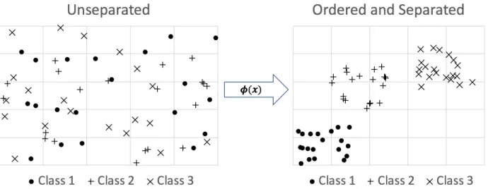
Figure 12 Ordered Separation of Classes ... 34

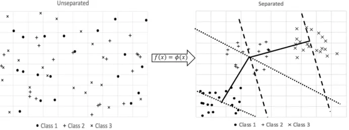
Figure 13 Separable Mapping 𝜙: ℝ2 → ℝ2. ... 36

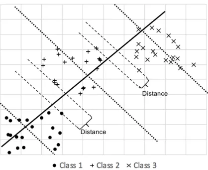
Figure 14 Parallel Hyperplanes. ... 38

Figure 15 Hyperplane Point Loss - Increasing Direction. ... 45

Figure 16 Hyperplane Point Loss - Decreasing Direction. ... 46

Figure 17 HPL for Three Ordinal Class Case. ... 47

Figure 26 OHPL as a Deep Neural Network: ... 50

Figure 27 Convolutional Neural Network Graph with OHPLnet Neural Network Layers ... 51

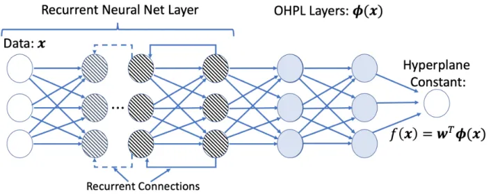
Figure 28 Recurrent Neural Network Graph with OHPLnet Neural Network Layers ... 51

Figure 18 Color Coded Confusion Matrix. ... 58

Figure 19 Time to Complete 500 Epochs by Number of Records (K records) ... 66

Figure 20 SWD Training Dataset: MZE and MAE vs Total Training Error ... 71

Figure 21 SWD Validation Dataset MZE and MAE vs Total Training Error ... 72

Figure 22 SWD Validation Dataset MZE and MAE vs Training Dataset MAE ... 73

Figure 23 SWD Validation Dataset MZE and MAE vs Training Dataset MZE ... 73

Figure 24 Validation Set MZE and MAE versus Training Set MAE ... 75

Figure 25 SWD Dataset Validation MAE, MZE and MAE + MZE vs Training set MAE + MZE. ... 95

Figure 29 Distribution of Row Pixel Count for Cropped Calcification Images ... 101

Figure 30 Distribution of Column Pixel Count for Cropped Calcification Images ... 101

Figure 31 Distribution of Row Pixel Count for ROI Calcification Images ... 101

Figure 32 Distribution of Column Pixel Count for ROI Calcification Images ... 101

Figure 33 Distribution of row pixel count for ROI Calcification Images with row pixel count between 700 and 1,100. ... 102

Figure 34 Distribution of column pixel count for ROI Calcification Images with column pixel count between 700 and 1,100. ... 102

Figure 35 Distribution of column pixel count for ROI Calcification Images ... 102

Figure 36 Sample Mammography Image ... 103

(21)

xix

Figure 40 Convolutional Neural Network Architecture ... 109 Figure 41 Training Data Mean Batch Error ... 110 Figure 42 NPS GRNN Network Graph ... 123

(22)

(23)

1

Chapter 1.

I

NTRODUCTION

The problem of ordinal class data occurs in a large and growing number of areas. Some of the most common sources and applications of ordinal data are:

• Ratings scales (e.g. Likert scales, star ratings), like customer satisfaction ratings, “promoter” ratings and quality ratings

• Sentiment scales (negative, neutral and positive)

• Medical classification scales of disease stage/severity/risk (mammogram image BI-RADS)

• Student performance (e.g., letter grades)

• Socio-Economic scale (e.g., high, medium and low)

• Meaningful groupings of continuous data (e.g., generational age groupings, grouping of noisy sensor data)

• Facial emotional intensity [1]

• Facial age estimation [2]

• Weather (e.g., storm severity classes)

• Performance ratings (e.g., high school prospects in football and basketball)

Historically, due to the high cost of data capture for sources like surveys, medical studies, etc., the vast majority of sources for ordinal data generated relatively small datasets (e.g., under 20K records of structured data or a hundred or less for unstructured data like medical images). In more recent years, there’s been a dramatic increase in the number of datasets and analysis problems, with ordinal classes as the primary output/focus, that have hundreds of thousands or

(24)

2

even millions of records are being analyzed. In addition, relatively large image and datasets, with ordinal labels are becoming common place. Many of these large data sets have their genesis in the explosion of use of digital and text data. Ratings surveys found on sites like Amazon and Yelp, large corporation Customer Satisfaction/Net Promoter surveys and the aggregation of medical history and/or imaging records into large data systems are primary examples.

Ordinal classes differ from nominal (unordered) classes by providing additional information/requirements in the form of a precise ordering of the classes. As a direct consequence, strategies for predicting nominal classes, tend to under-perform when applied to ordinal data. The use of sequential integers to represent the ordered classes is natural and commonly used for labeling the ordered classes. This representation might suggest that the application of methodologies like regression, that attempt to predict a continuous value would be effective in developing ordinal classifiers. Strategies like regression assume that equal “distances” between values have a consistent numerical meaning (e.g., all one-unit differences having the same meaning), but this assumption is rarely true in ordinal data. Within prediction algorithms, these fundamental differences in the type of data being predicted may be addressed in the loss function or by employing potentially complex, multi-model strategies. An ideal loss metric for ordinal classification would assess the ordering of the data and form discrete homogeneous class groupings without imposing an equal “distance” assumption between predicted classes.

The fundamental difference in ordinal and nominal classes also leads to a difference in assessment for classifier performance. The best classification strategies must not only have a classification accuracy that is on par with or better than other strategies, but in the best strategies

(25)

3

misclassified cases should to be ‘close’ to the correct class (e.g., misclassifying a ‘3’ as a value of ‘4’ is more desirable than misclassifying it as a ‘5’).

Existing strategies to address the unique requirements of classifying ordinal data utilize the power of methodologies like SVM (Support Vector Machines) [3, 4, 5, 6, 7] and Gaussian Processes [8]. Others that use Deep Neural Networks employ complex multi-model or repeated-sampling approaches. As such, any attempts to apply them to the large datasets would require major alterations to the algorithm or the use of complex sampling or ensemble strategies that are applied to nonlinear model results.

To address these conditions unique to the ordinal classification problem (also known as the ordinal “regression”), the Ordinal Hyperplane Loss (OHPL) was developed by addressing the following algorithm goals for a current ordinal labelled class of the training data:

1) develop a Neural Network to define a nonlinear mapping of the data into a vector valued output space

2) train the network to establish and maintain the ordering of the classes 3) “drawing” like labelled samples closer together

This formulation maintains the ordering without imposing assumptions regarding the distance between different classes (e.g., as would be imposed by using ordinary least-squares regression analysis). At the same time, the algorithms that are developed from this approach can be applied to very large classification problems.

The remainder of the thesis is organized as follows. Chapter 2 reviews relevant work and existing algorithms, that attempt to solve the ordinal classification problem. Chapter 3 provides

(26)

4

a review of Deep Learning including variants of Artificial Neural Networks and related considerations in using Deep Learning algorithms to solve classification problems such as Ordinal Classification. Chapters 4 and 5 cover the geometric and mathematical framework for the development of Ordinal Hyperplane Loss (OHPL). Chapter 6 documents experimental results for the original OHPL work. OHPLall is the culmination of work that’s focused on improving upon the original OHPL methodology for application to very large datasets. These advances are reported in Chapter 7. A successive series of algorithm strategies that were designed and tested to improve algorithm performance both in terms of speed and accuracy of predictions are reported in Chapter 8. Chapters , while Chapters 8 through 10 review three different applications of OHPL and OHPLall. Chapter 11 contains conclusions from this work.

(27)

5

Chapter 2.

L

ITERATURE

S

TUDIES

In January 2016, Gutierrez, et. al. published an extensive examination of solutions to the Ordinal Classification problem [9], including benchmark performance metrics versus a set of standard datasets that were included in the work of Chu and Ghahramani [8]. In their review Gutierrez et. al. grouped the existing top performing methodologies into three categories that address the Ordinal Classification problem: 1) Naïve Approaches, 2) Ordinal Binary Decompositions and 3) Threshold Models. While their work attempts to provide a framework for three distinct classes of models, the team acknowledges that many of the most common approaches could be classified into more than one category. Unless specifically attributed to a different researcher, the content of the remainder of this section is attributed to the work of Gutierrez, et. al. [9].

Naïve approaches use an appropriate simplifying assumption to re-cast the problem in such a manner that existing methodologies can be applied. If the researcher assumes that the difference in classes is “close” to uniform they may transform the classes into sequential integers and apply regression analysis like ordinary least squares, neural networks or SVR (Support Vector Regression). Cost sensitive methodologies which use different weights for different misclassification types also fall into this category. Another common naïve approach ignores the class ordering by applying nominal classification approaches like SoftMax regression or multi-class SVM, to predict multi-class membership.

Cost sensitive classification is a more advanced naïve approach. In this approach, misclassification costs will differ between two or more classes, with a goal of maximizing accurate

(28)

6

classification of the most desired class. Support Vector Machines with Ordered Partitions (SVMOP) is a high performing algorithm that falls in this category [10]. The algorithm uses class differences, as weights, in an effort to not only provide correct classification, but to encourage misclassifications that are close in class number to the actual class (e.g., for an actual class value of ‘2’, the algorithm encourages a miss of ‘3’, instead of a ‘5’).

The fundamental basis of binary decomposition is to recast the problem as a set of binary classification problems. The problem may be posed by comparing pairs of ordinal values with the higher value being assigned a value of 1 and then using either a single or multiple binary classification models. In the case of multiple classifiers, the analyst may produce as few as k-1

classifiers for k ordered classes or as many as &𝑘₂( =*₊𝑘 ∗ (𝑘 − 1) classifiers (i.e., all ordered pairs). An appropriate decision rule is then applied to the set of classifiers. In the k-1 case, each adjacent ordered pair is analyzed as a binary problem. One popular process examines the highest value in a sequence of values that meet a minimum model value threshold. For example, assume that we have five ordinal classes: ‘1’, ‘2’, ‘3’, ‘4’ and ‘5’. If the first three classifiers (‘1’ vs ‘2’, ‘2’ vs ‘3’ and ‘3’ vs ‘4’) estimate values of 0.5 or higher, but the fourth (‘4’ vs ‘5’) does not, it results in a classification of the highest of the first three classifiers (or ‘4’, in this example). If the first binary classifier value does not meet the threshold of 0.5, then the record is classified as the lowest ordinal value (’1’ in the example). Similarly, the analyst may choose to group classes based on classes (e.g., ‘1’ vs ‘2’-‘5’, ‘1’ & ‘2’ vs ‘3’–‘5’, ‘1’-‘3’ vs ‘4’ & ‘5’ and ‘1’-‘4’ vs ‘5’).

The earliest ordinal binary decomposition approaches used Ordinal Logistic Regression [11], employs logistic regression to estimate the binary probabilities for class ordering (e.g., probability

(29)

7

that the label for a given record is ‘3’ or higher). More recent binary decomposition strategies use machine learning approaches like Support Vector Machine (SVM) algorithms to create individual binary classifiers, combined with classification strategy using the binary classifiers. Deep Neural Networks allow of the output of multiple estimates. These estimates may be used to create class probabilities for all classes in a single model. Some approaches endeavored to use non-parallel hyperplanes, in an SVM framework, but at a high cost of increased model complexity. Note that SVMOP would fit into the binary decomposition category but is more appropriately classified as a cost sensitive methodology, within naïve approaches.

A new variant of Ordinal Regression was proposed by Cheng et. al., in 2007. In this approach, a single Deep Neural Network is used to predict the classes. Their approach is very similar to a multilabel classification problem using a DNN, where multiple outputs are estimated with all elements of the output layer being the value from a sigmoid function [12]. To set up the analysis for k ordinal classes, the label value for each record is recoded into a k-1 length vector. For a given class value, ‘a,’ all index values of the vector with position value (using the standard 0 index value for the 1st_{position in the vector) that are less than ‘a’ minus the minimum ordinal value are}

coded with a 1. All other values are coded with a zero [12].

The three ordinal class case, with ordinal values ‘1’, ‘2’ and ‘3’, is illustrated in Table 1. For the three-class problem, the neural network essentially estimates two binary models. The first output predicts the likelihood that the label is greater than ‘1’, and the second one predicts the likelihood that the label is greater than ‘2.’ Once the algorithm converges or reaches a predefined stopping point, a classification rule, typically whether or not the value is greater than 0.5, converts each output vector into a binary array that is similar to the one used for training. Ordinal classes are

(30)

8

assigned based on which encoded vector matches the binary output. If the first position is zero, then the record is assigned the value of the minimum label [12].

Table 1 Ordinal Regression Three Class Label Encoding

Label Vector

1 [ 0, 0 ]

2 [ 1, 0 ]

3 [ 1, 1 ]

It should be noted that, while the vast majority of class predictions will conform to one of the vector values of the encoded ordinal classes, it is possible for vector values that do not conform to exist. In the three-class problem, it is possible to have a prediction of ‘[ 0, 1 ]’ from applying the resulting model to a data record (either in the training set, a test or validation set or to completely new data). It is left to the analyst to determine how to classify these nonconforming results.

Threshold models are comprised of a large number of methodologies including:

1. Cumulative Link Models: Traced to the Proportional Odds Models that were originally created in the 1980s. Cumulative Link Models map the input data into a one dimensional (i.e., a number line). This number line is appropriately partitioned, to provide class predictions.

2. Support Vector Machines: In 1999, Herbrich et. al. developed single model SVM approach that transformed the input data by calculating the difference between pairs and used the sign of the ordinal class differences. Other applications involve pointwise approaches that

(31)

9

produce k-1 hyperplanes, to classify k ordinal classes. Given the simple ordering information that is available, with ordinal data, the problem lends itself well to algorithms that uses distance learning principles. In 2005, Chu & Keerthi developed two SVM algorithms that specifically address the ordinal classification problem through the estimated multiple hyperplanes that maintain the sequential ordering of the classes [5]. While successful in application to small datasets, their algorithm converts the original SVM proposed by Vapnik et. al., that has a unique individual constraint, for every record, in the dataset, into an optimization problem that has (k-1)*n constraints. Keerthi et. al.’s more effective algorithm, which they call ’IMC,’ has a problem size of (k-1)*n, while the ‘EXC’ variant scales to a problem size of 2n+k [5]. The most efficient SVM algorithms have a computational cost of 𝒪(𝑛+_)._{This computational cost tends to make SVMs impractical} with large datasets. Scaling the problem size by a factor of two would quadruple compute cost. For problems with 10 or more classes, the cost for IMC would increase by a factor of 100 or more.

3. Discriminant Learning: The models maximize between class differences and minimize within class differences using the variance-covariance matrix and the Rayleigh coefficient. To adapt discriminant analysis to the ordinal classification problem, an ordering constraint is applied over the contiguous classes. SVM falls under a broader context of kernel methods. Cardoso et. al., in 2012, developed a set of three Kernel Discriminant Analysis (KDA) base ordinal classifiers [13]. One of the classifiers extends the work Frank and Hall, in 2001, which employs a series of binary classifiers [14]. The second uses the data replication strategy of Pinto da Costa, et. al., in 2005 [15]. The third strategy involves the

(32)

10

development of a modified Kernel Discriminant Analysis which applies an ordering constraint on the projected means.

4. Augmented Binary Classification: The general framework includes the development of multiple samples from the original sample, including a weighting of the samples. A binary classifier is then developed using the full set of multiple samples (any binary classification algorithm can be used). Lastly, a ranking process is constructed using the output of the binary classifiers. Pinto da Costa et. al. developed a data replication strategy to design an ordinal classifier that utilizes Deep Neural Networks (DNNs) [15]. In their work they utilized an additional data dimension that represented the sample orderings (e.g., ‘0’ vs ‘1’ and higher has a value of 0, in the additional dimension while ‘0’ & ‘1’ vs ‘2’ and higher had a value of 1). In work that was published in published in 2010, the researchers successfully extended their work data replication strategy, into SVM applications [16]. One of the most common of the distance learning methodologies is Support Vector Machines, which seek to identify hyperplanes that separates classes, in a higher dimensional space. As such they are a natural machine learning methodology to apply to ordinal classification problems. 5. Ensemble Models: The RankBoost algorithm attempts to improve a set of confidence

functions, that maximize an ensemble of binary classifiers. Similarly, the ORBoost algorithm applies the same concepts to develop improved performance from ordinal regression models. The basic framework for the creation of ensemble models is the development of “weak” classifiers, that are combined to produce an algorithm that outperforms each of its components. Ensemble methods have a documented history of outperforming competing single model solutions. The weak classifiers may be generated

(33)

11

by using a subset of available features, a subset of records (usually bootstrap sampling) or some combination of the two. Instead of determining an optimal combination from a full set of weak classifiers, boosting algorithms begin with an initial classifier, then add additional weak classifiers until incremental classifier improvement (e.g., improvement in model accuracy, on the training set), becomes zero (or approaches zero).

6. Gaussian Process: GPOR uses a Bayesian framework to model a latent function via Gaussian Processes. Prior and posterior probabilities for class membership are estimated for a set of latent functions of the input features. Optimization with respect to the hyperparameters results in probability estimates of class membership, based on the input record. GPORs include an optimization algorithm that discovers the ideal thresholds for classifying data records based on the output metric, from the gaussian process. GPOR is an example of an analytic framework that could fit into multiple categories.

In late 2016, Hamsici and Martinez proposed a Support Vector Machine based algorithm that attempted to maximize the margins between adjacent classes [17]. The authors apply Sequential Minimal Optimization (SMO), to efficiently and simultaneously solve k-1 problems, where k is the number of ordinal classes. Their algorithm is similar to that Keerthi and Chu, but with the notable and meaningful difference that their algorithm does not assume equal margins between adjacent classes. In addition, their algorithm includes weight parameters, that enable the prioritization of one or more of the individual algorithms, over others. This prioritization weighting allows a researcher to focus on a specific pair of ordered classes (e.g., a medical researcher may want the classifier to have the best possible classification of stage two cancer versus stage three, while still

(34)

12

effectively classifying five different ordinal classes). Weighting can also be used to address unbalanced classes within the data (i.e., unbalance records counts for the classes).

In 2017, Wang, et. al. used a nonparallel hyperplane assumption for the development of a specialized Support Vector Machine (SVM) algorithm to address the Ordinal classification problem [7]. For k ordinal classes, their algorithm estimates k-1 hyperplanes. For each, they include constraints which ensure that like-labelled samples are within a prescribed margin of the hyperplane, while unlike-labelled samples are one or more units away. They also include constraints to ensure the ordering of the hyperplanes reflect the ordering of the classes. The use of nonparallel hyperplanes may result in classification issues, if data points map into a region near the crossing of two hyperplanes.

These algorithms exhibit mixed performance across the standard test data sets that are used to benchmark performance of ordinal classifiers. Many are benchmarked using 20 or more small datasets, with performance that represents modest improvements, when the algorithm actually outperforms other classifiers. While these incremental improvements are notable, they are being benchmarked against current “best in breed” classifiers, so as a rule, it is rare to find one that outperforms best benchmark classifier by 10% or more in terms of decline in classification error. It is worthy of note, because the solution that is reported in Chapter 5 has an accuracy improvement of fourteen percent or more on two out of seven benchmark datasets, when compared to four of the highest performing algorithms.

In February 2018, Nguyen et. al. incorporated “Triplet Loss” based constraints to an algorithm that is similar to SVM optimization [3]. Their algorithm employs triplet loss-based constraints, on local clusters of data points. The researchers produced a linear version of their algorithm, as well

(35)

13

as a version that employs the kernel trick to produce a nonlinear mapping of the data into a higher dimensional space. Within their work, the algorithm produced solid results with mixed performance where the linear version outperformed the nonlinear version roughly half of the time. Given the researcher’s stated algorithm compute cost of 𝒪(𝑛3₎_{, while their solution is} successful with relatively small datasets (e.g., under 25,000 records), it may not be viable for larger datasets. In the future, they could conceivably develop a new version that uses SMO to solve the problem, once the constraints are developed. Doing so should broaden the applicability to larger datasets, but still may not be viable if the number of records exceeds 100,000 by a significant amount.

Triplet Loss is a term that was first used in the ground-breaking FaceNet solution to the ReId (reidentification) problem [18]. In developing FaceNet, Schroff et. al. leveraged the foundational work in Large Margin Nearest Neighbor (LMNN) Classification published by Weinberger and Saul [19]. The essence of the FaceNet process is to train a Convolutional Neural Network (CNN) to produce an N-dimension embedding, that is optimized based on relative distances of similar and dissimilar pairs of data points. A margin, that is analogous to the margin found in a Support Vector Machine, is used to ensure that similar pairs (those with the same label) being “closer” than dissimilar pairs (those with different labels) is based on a difference in distances that is not trivial (i.e., not arbitrarily close to zero). This process produces what is commonly called a “triplet loss” function (discussed further in Chapter 4) that is based on linear distance comparisons. As the following general triplet loss function demonstrates, the loss function uses a fixed margin that is strictly greater than zero, to ensure that a point, 𝒙5, is closer to the positive anchor, 𝒙6 (same

(36)

14

class), than it is to the negative anchor, 𝒙7 (different class from 𝒙5) and the difference, 𝛿, is fixed and not trivially close to zero [18].

𝑡𝑟𝑖𝑝𝑙𝑒𝑡 𝑙𝑜𝑠𝑠 = maxF𝑑F𝑥₆, 𝑥₅I − 𝑑(𝑥₇, 𝑥₅) + 𝛿, 0I (1)

Triplet loss puts a significant burden on the analyst to devise a reasonable strategy for identifying triplets for use in estimating function error, since the number of possible triplets grows as a cubic function of dataset size [20]. The framework of triplet loss provides a mechanism for applying a distance comparison between points without requiring the underlying distance assumptions of regression analysis. This framework of triplet loss makes it well suited to the ordinal classification problem, but triplet loss cannot be used because it does not guarantee that the ordering information is utilized nor that the ordering of classes is guaranteed (it only guarantees that different classes are separated). While it cannot be directly applied, triplet loss provides some of the intuitive motivation for methodology reported in Chapter 4.

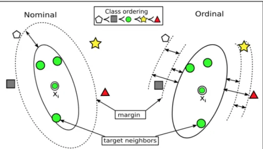
Triplet loss effectively addresses the ordering, but only as it relates to an identified triplet of data points. In developing LODML, Nguyen et. al. developed a useful geometric representation of the goal of their use of triplet-based constraints. In a two-dimensional representation of a neighborhood, they illustrate the goal of classes falling in ‘distance band’ radiating out from the center of the neighborhood with the center being a chosen data point (Figure 1, below) [3]. In comparing a nominal problem, to an ordinal problem their graphic illustrates that the ‘distance’ frame of reference must be rotated, to ensure that the ordering of classes to be properly maintained. Without loss of generality, these distances could easily be mapped to a continuous scalar scale. In doing so, the ordered classes would occur in clusters along the number line.

(37)

15

Figure 1 Local Neighborhood Ordered Classes vs Nominal Classes

The image on the left illustrates distance metric learning for the nominal classification problem. The image on the right illustrates the ordinal classification problem [3]

(38)

16

Chapter 3.

D

EEP

L

EARNING

Deep Learning falls under the broad class of Artificial Neural Networks (ANNs), which have origins that date back to the 1800s [21]. With its origins from simple Multi-Layer Perceptrons, Deep Learning is one of the primary Machine Learning strategies that are in wide use throughout the world with a history of solving a broad variety of data analysis and classification problems. Deep Learning is made up of a number of specialized classification strategies that have been derived from Deep Neural Networks (DNNs) which may also be called Artificial Neural Networks (ANN). DNNs originate from the Multi-Layer Perceptron, with the DNNs primary distinction as having a greater degree of complexity due to having more hidden layers and more nodes.

Like other machine learning methodologies, the application of Deep Learning algorithms falls into two general categories based on the “goal” of the application. Supervised applications have a targeted outcome that the algorithm attempts to predict based on other existing data. This targeted outcome is separate from the data that is being used for prediction. Examples of supervised problems are the prediction of category (class) membership (e.g., predict whether or not a picture has a dog in it) or predicting a volumetric outcome (e.g., how much money will a customer spend in the future). Unsupervised applications focus on the development of insight or understanding of the data without having a specific target with which the outcome may be compared to determine the accuracy of the mathematical model that is developed. Examples of unsupervised applications are data reduction techniques (e.g., autoencoders) which attempt to capture as much “information” from the existing data in a significantly fewer number of data elements. Unsupervised applications also include various forms of cluster analysis, which attempt

(39)

17

to group data records into homogeneous sets while providing maximum separation between the groupings [21].

3.1.

T

HE

M

ULTI

-L

AYER

P

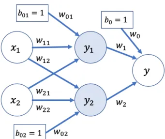
ERCEPTRON

Figure 2 is a basic visual representation of a Multi-Layer Perceptron (MLP). The columns of circles are called a “layer” and each circle is called a “node.” The arrows that connect the nodes represent numerical weights, that are calculated during the model estimation process. The dashed arrows represent a feedback process, that incrementally updates the weight values, through a process called “Back Propagation.”

Figure 2 Simple Multi-Layer Perceptron with weight updates

The nodes also represent a nonlinear transformation of the input data, called the “activation function”, after they are multiplied by their respective weights and summed. The activation functions provide the nonlinearity to the algorithm’s learning process. Ideal activation functions

(40)

18

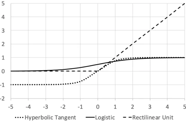
are sufficiently simple and well behaved to allow the numerical estimation and update processes that are required for learning. Figure 3 includes the graphical representation of three of most common activation functions [22]:

Sigmoid Function (AKA Logistic Function): 1

1 + 𝑒Z[ (2𝑎)

Rectified Linear Unit (ReLU): max(𝑥, 0) (2𝑏) Hyperbolic Tangent (tanh): 𝑒_𝑒[_[ − 𝑒_{+ 𝑒}Z[_Z[ (2𝑐)

Figure 3 Plot of three common activation functions, found in Deep Neural Networks

As a general rule, Neural Networks, including MLPs, are initialized with small random weights. Each record of data is then fed through each node, by applying the corresponding weights, summing and then applying the activation function for the node. This process occurs in each

(41)

19

node, layer by layer until the final output (output layer) is reached. At this point, the loss (i.e., classification error) value is calculated by comparing the output value to the “ground truth” that is represented by the label or target value for the individual data record. One of the most common loss functions is the summed squared error. If we denote the algorithm output as 𝑦l and the ground truth value as 𝑦 then the summed squared error for a DNN that is applied to dataset D, would be:

𝑆𝑢𝑚𝑚𝑒𝑑 𝑆𝑞𝑢𝑎𝑟𝑒𝑑 𝐸𝑟𝑟𝑜𝑟 = r(𝑦5 − 𝑦l5)+

5∈t

(3)

The weight values within each of the nodes are then updated via backwards propagation, represented by the curved dashed arrows, in Figure 2. The numerical basis for the weight updates is based on Stochastic Gradient Descent (SGD), which calculates the optimal update value via the application of partial derivatives, with respect to the respective weight values for the composition of activation functions that lead from the node to the output layer. Unlike Total Gradient Descent, which applies updates after all training records are fed through the neural network, Stochastic Gradient Descent, updates with each record [23]. However, in most cases today, SGD is applied to mini-batches of records to promote stability in estimating the gradient [21]. An explicit example of this weight update process is given in the Exclusive OR section (see Section 3.2).

When applied to data, SGD is calculated by using the sum of values across a sampling of the data. In real applications, SGD is not what is used in most Deep Learning algorithms [22]. Newer methodologies like Adam have a foundation in SGD, but address some of the issues of applying SGD to small batches and combining the result with prior weight update values, which leads to faster convergence of algorithms [24]. After the weights are updated, the process repeats.

(42)

20

One of the outputs of successive iterations of a DNN is a sequence of scalar value, that represents the total cost (error in estimation) for the iteration.

Definition1: 𝐹𝑜𝑟 𝑎₇ ∈ 𝑠𝑒𝑞𝑢𝑒𝑛𝑐𝑒 𝐴, 𝑖𝑓 𝑡ℎ𝑒𝑟𝑒 𝑒𝑥𝑖𝑠𝑡𝑠 𝑎∗_{𝑤ℎ𝑒𝑟𝑒 𝑓𝑜𝑟 𝑔𝑖𝑣𝑒𝑛 𝜀 > 0 𝑎𝑛𝑑}

𝑎𝑙𝑙 𝑖 ≥ 𝑛 𝑎𝑏𝑜𝑣𝑒 𝑎 𝑡ℎ𝑟𝑒𝑠ℎ𝑜𝑙𝑑, |𝑎5 − 𝑎∗| < 𝜀, 𝑡ℎ𝑒𝑛 𝑡ℎ𝑒 𝑠𝑒𝑞𝑢𝑒𝑛𝑐𝑒 𝑖𝑠 𝑠𝑎𝑖𝑑 𝑡𝑜 𝑐𝑜𝑛𝑣𝑒𝑟𝑔𝑒

𝑡𝑜 𝑎∗_[25].

From a practical application, individual machine learning algorithms are not tested for this formal version of convergence, but the basic principle is applied. When the algorithm reaches the point that improvement in the cost function value ceases to occur or improvements are trivially small, the algorithm is said to have converged.

3.2.

T

HE

E

XCLUSIVE

OR

PROBLEM

(XOR)

The Exclusive OR (XOR) problem represents one of the simplest classification examples, where the labeled outcomes are not linearly separable in the space of available predictive attributes. The problem has four records with two attributes, 𝑥_* and 𝑥₊ [26]. The labels of ‘AND’ represent combinations of 𝑥_* and 𝑥₊ that are equal, while the desired labels of ‘OR’ will have a value of ‘1’ for 𝑥_* or 𝑥₊, but not both and ‘0’ for the non-one (see Table 2). Geometrically speaking, the four records represent the corners of a box in two-dimensional space. In Figure 4, the desired ‘OR’ cases are represented by solid dots, while the ‘And’ case are circles. As illustrated in the figure, a circular shaped threshold provides the separation of the cases that is desired for the problem [26].

(43)

21

Table 2 XOR Data

Label 𝑥* 𝑥+ y

AND 0 0 0

OR 1 0 1

OR 0 1 1

AND 1 1 0

Figure 4 XOR Plot

To solve the problem, the labels are converted to binary 0 and 1 values (i.e., the ‘y’ values in the table), since algorithms cannot use text directly. It can also be noted that

𝑦 = 𝑓(𝑥_*, 𝑥₊) = 1 − (𝑥_*+ 𝑥₊− 1)+₍₃₎

provides a perfect solution to the problem, but the vast majority of classification problems cannot be solved via simple visual inspection and educated guessing of a solution. If traditional statistical methodologies were used to attempt to provide a numerical formula to solve the problem, the analyst may attempt to fit a function of the form

𝑦 = 𝑓(𝑥*, 𝑥+) = 𝑎𝑥*++ 𝑏𝑥+++ 𝑐𝑥*𝑥++ 𝑑𝑥*+ 𝑒𝑥++ g (4)

where ‘a’-‘e’, ‘g’ in (4) represent the unknown coefficients that the methodology would attempt to estimate to improve model fit. This framing of the problem results in four data points, with six unknowns, so no unique solution is possible. As such, classical statistical methodologies that are commonly applied would not work for solving the problem. As a direct consequence, the XOR problem may be the simplest problem that requires the nonlinear estimation power that is presented by ANNs.

(44)

22

Figure 5: Fully Annotated XOR Neural Network Graph

Figure 5 represents the fully annotated network graph for solving the XOR problem. The boxes with 1’s represent the constant or “bias” terms ( 𝑤_„′s) that need to be estimated along with the weights for the data elements. They were omitted from Figure 2, to provide a simplified visual introduction to neural networks. To solve the XOR problem, the process starts by using random values for the weight and bias. After each submission of the data points through the neural network is completed, the “loss” value, 𝐿 is calculated, by summing the squared difference between the predicted value 𝑦l and the correct label 𝑦 as the error value [22]

𝐿 = r(𝑦 − 𝑦l)+_{. (5)}

The gradients that are used for the weight updates are the partial derivatives with respect to the given weight and bias value. The sigmoid function is used as the node activation function (nodes 𝑦_* and 𝑦₊) and is represented as 𝜎_* and 𝜎₊ in equations (6) and (7). For each weight or bias value and for each data record 𝑛 (represented by row number) the ANN update process uses the partial derivatives with respect to the weight (or bias value). The update for the output layer is [22]

(45)

23

For 𝑖 ∈ {0, 1, 2} representing the hidden layer node:

𝜕𝐿 𝜕𝑤₅ = r 𝜕(𝑦₇− 𝑦l₇)+ 𝜕𝑤₅ • 7Ž* = r 2(𝑦7 − 𝑦l7) • 7Ž* 𝑦„,7 (6) The updates for the hidden layer (nodes y1 and y2) are a little more complicated (see equation (7)).

For 𝑗 ∈ {0, 1, 2} and 𝑖 ∈ {1, 2}, representing the data source and hidden layer nodes, respectively: 𝜕𝐿 𝜕𝑤_‘,5 = r 𝜕(𝑦₇− 𝑦l₇)+ 𝜕𝑤_‘,5 • 7Ž* = r 2(𝑦₇− 𝑦l₇) • 7Ž* 𝜕𝜎_5,7 𝜕𝑤_‘,5 = r 2(𝑦7− 𝑦l7)𝜎5,7F1 − 𝜎5,7I𝑥‘,7 • 7Ž* (7)

Note that equation (7) is effectively equation (6) with an added term, to represent the gradient from the output of the hidden layer to the input layer of the data. This chaining of gradient components has potentially serious implications if a large number of hidden layers are used in the neural network.

The gradients represent the direction and magnitude for increasing value at the current state of the system. To reduce the error terms the gradients are subtracted from the weights. As a general rule, a step size or “learning rate” is applied to the gradient before it is subtracted from the weight. Adjusting the step size can lead to a more efficient convergence to an optimal solution. Note that excessively large step sizes may even prevent the algorithm from achieving an optimal solution.

(46)

24

3.3.

D

EEP

N

EURAL

N

ETWORKS

The most basic form of Deep Learning is a form of supervised learning called Deep Neural Networks. They are distinguished from simple MLP’s in the number of hidden layers that are utilized. This deeper architecture comes with its own challenges. The calculated gradients may explode in size or vanish, if the multiplicative chain in the calculation has sufficiently large or small values, respectively, at each point in the chain [21].

Figure 6 DNN Representative Graph

There are a number of strategies that may be employed to address this issue. For a period of time, the pretraining of network layers, using unsupervised learning techniques to establish initial weights then using back propagation to refine the weights for the full network was a useful strategy. More current architecture designs use Rectified Linear Units (ReLU) as the activation function to address the problem. In addition to minimizing the likelihood of vanishing/exploding gradients, the use of ReLU as the activation function in DNN nodes has also been demonstrated to improve algorithm performance [21].

(47)

25

For extremely deep neural networks, the use of ReLU activation functions does not always solve the vanishing/exploding gradient problem. Residual Neural Networks include additional connections in the graph that skip layers. These networks were used to handle very deep image classification problems with exceptional performance [27].

Figure 7: Residual Neural Network Graph

Deep neural networks are also applied to more challenging problems like image classification. The most obvious challenge in attempting to classify images, is the structure of the data itself. Images are two-dimensional if grey scale or three-dimensional if they are in color (e.g., a color image with red, green and blue layers). Reformatting an image to a one-dimensional array removes a significant amount of information from the data.

The standard approach to address image classification is the use of a Convolution Neural Network (CNN). In this approach, images are analyzed by systematically assessing small overlapping “patches” of the image (two-dimensional subsets of the image; if color then three-dimensional). Much like the input to output process for a DNN node, a set of weights is applied to the data, in the patch, which are summed, and a nonlinear activation function is applied. Each

(48)

26

set of weights and activation function that is applied, in a pass over an image is called a “filter” to create a dimensional output. The application of multiple filters results in multiple two-dimensional outputs (called “channels”). A single “convolution” layer applies multiple filters producing a three-dimensional data object that is many times deeper than the original image (or prior layer output; see Figure 8). The data are then “pooled”, typically by taking the maximum value of a patch of the output channels (which may differ in size from the convolutional layer patches), to reduce the volume of data. Each patch is applied independently in a convolutional layer. Weights for the filters are updated across the entire layer (and mini-batch). Multiple iterations of convolutions and pooling may occur within an algorithm. At the end of these iterations, the data are reformed into a one-dimensional vector (the “Embedding” in Figure 8), that is then fed into a standard DNN layers [28].

Figure 8 Basic Convolutional Neural Network Graph

A number of highly successful, general purpose CNNs are available for image classification. These CNNs are pretrained on very large image datasets and can be used to simply preprocess

(49)

27

image data into the final one-dimensional layer or may be used as a pretrained CNN that refines the network weights through a training session. Examples of these pretrained CNNs are VGG16, ResNet50, AlexNet, GoogleNet and InceptionV3 [27, 29, 30, 31, 32].

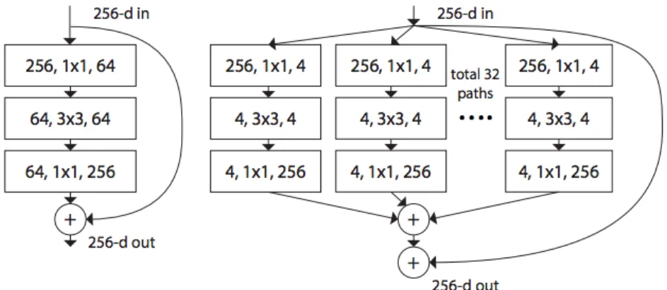
The next generation of ResNet image classifier called “ResNeXt” [33]. Figure 9 comes from the publish paper by Xie, et. al. A key differentiator of ResNeXt and ResNet is the use of multiple parallel paths, which contain their own convolution and pooling layers as well as the inclusion of a residual path (essentially a second independent path of hidden layers from some output layer that is rejoined later in the neural network) [33]. The residual path may have the same architecture as the other path(s), but it also may differ. Before the two paths are joined their data structures must match, so great care must be taken in creating the residual paths [33].

Figure 9: ResNeXt versus ResNet Architecture Fundamental Differences

Left: A block of ResNet. Right: A block of ResNeXt with cardinality=32. Layers shown as: # in channels, # out channels. Complexity is essentially equal [33]

One of the most complex Deep Learning algorithms is the Recurrent Neural Network or RNN. From a basic design point, the RNN graph is similar to a DNN. The difference in design comes from the recurrent connections which feed data backwards to an earlier layer within the network (Figure 10). This recurrence process makes RNNs well suited to handling time series or sequence

(50)

28

data. The RNN may have a full DNN as the last layers of the network, or it may have a last layer that simply feeds the output layer [34].

Figure 10 Recurrent Neural Network Graph

A useful type of unsupervised learning that comes from the Deep Learning is the Autoencoder. The goal of these neural networks is to reduce data dimensions (number features). They take an input dataset and process it through one or more hidden layers, that have significantly fewer nodes than the number of input features. The output layer has the same number of nodes as the number of input features. The input and output nodes are paired one to one. The loss function is the sum of the squared differences for the pairings [21]. Since the goal of the process is to reduce data dimensions, the number of nodes is usually significantly smaller than the number of input features. When training is completed, the layer with the smallest number of nodes represents the reduced data dimensions. Figure 11 is a simple representation, but auto encoders may have a deep architecture, particularly for extremely large data sources.

(51)

29

Figure 11 Simple Autoencoder

3.4.

M

INI

-B

ATCH

P

ROCESSING

Deep neural network algorithms have a computation complexity of 𝒪(𝑛“₎_{[35]. As data set} size, increases to today’s “Big Data” levels of millions or billions of rows of data, the computation complexity, in submitting the entire dataset, in a single pass through the DNN is not possible. DNNs almost always use some form of small batch or mini-batch submission process. For a batch size b, that is significantly smaller than the full dataset size, the computation complexity of submitting a single batch is 𝒪(𝑏“₎_{. To submit all of the data in a data set with}_n_records,_{𝑐𝑒𝑖𝑙(𝑛/𝑏)} submissions must occur, so the computation complexity of submitting the full dataset, one time using mini-batchers is

𝒪(𝑏“_{) ∗ 𝑐𝑒𝑖𝑙 &}𝑛

(52)

30

𝒪(𝑏•₎_{is a constant, meaning the use of mini-batches takes an algorithm that has a computation} complexity of 𝒪(𝑛“₎_{and makes the problem linear in terms of number of records,}_𝒪(𝑛)_{. In} addition, the use of mini-batches has demonstrated improved generalizability of deep neural network models [36].

3.5.

H

INGE

L

OSS

Support Vector Machines were introduced by Vapnik et. al. in the mid 1990’s [37]. While the name did not originate until sometime later, they created the concept of “hinge loss”. For the vast majority of datasets that are not perfectly separable, the “soft margin” version was introduced that introduced a constraint of the form:

𝑦₅(𝒘˜_𝒙

5 + 𝑏) ≥ 1 − 𝜁5, 𝜁5 ≥ 0 (1)

Where 1, on the right-hand side, is the “margin” associate with the loss function (the margin can be set to a value of 1, without loss in generality). A more general version of this inequality, with nonzero margin, 𝛾, could be expressed as:

𝑦₅(𝒘˜_𝒙

5 + 𝑏) ≥ 𝛾 − 𝜁5, 𝜁5 ≥ 0, 𝛾 > 0 (2) It can be shown that this system of inequalities is equivalent to:

𝜁₅ = max(𝛾 − 𝑦₅(𝒘˜_𝒙

5 + 𝑏), 0) (3)

This equation is the essence of the Hinge Loss function, where loss is zero, for function values below zero and loss contribution occurs when the function is above zero. For at least the past decade, Hinge Loss is one of the most common loss functions used in deep learning algorithms. This functional form is important in the creation and application of Ordinal Hyperplane Loss

(53)

31

(OHPL), where a simple linear difference of scalar values contributes to algorithm loss (error). If the value of the difference is positive the loss is set to that value. If not, it is set to zero. This function is continuous for all 𝒙 and differentiable for all 𝒙, except when 𝒘˜_𝒙

5 = −𝑏. Triplet Loss is a special application of Hinge Loss, that uses the difference in distance from a single point (called the positive anchor) to two other points, one of which has the same label as the positive anchor and the other has a different label. The value is zero unless the point with the unmatched label is not sufficiently further away from the anchor point, than the matched label point, by a preset margin. This function provides an easy way to focus deep net training, on “hard cases” that are a significant distance from the desired goal, while setting the distance, for cases that are close to the goal, to a value of zero. In developing OHPL, the underlying principles of Triplet Loss and Hinge Loss are combined, to develop a special loss function that directly addresses ordinal classification problem.

(54)

32

Chapter 4.

O

RDINAL

C

LASSIFICATION

P

ROBLEM

D

ESCRIPTION

This chapter covers the proposed solution to the Ordinal Classification problem that utilizes deep learning to directly develop a classification metric, a relatively intuitive mathematical and geometric motivation for the solution. The proposed strategy employs a commonly applied functional form that is used to develop large margin classifiers in machine learning. Conceptually, these frames of reference provide a foundation for the development of a unique loss function, that enables the application of virtually any deep learning architecture (DNN, CNN, RNN, etc.) to solve ordinal classification problems [38].

4.1.

F

UNDAMENTAL

O

RDINAL

C

LASSIFICATION

P

ROBLEM

The proposed solution focuses on the identification or estimation of a nonlinear mapping,

𝜙(𝑥), that provides an optimal separation of classes, with three fundamental properties.

1. Different classes must be properly ordered. Numerically, they can be separated in either increasing order or decreasing but they must be properly ordered. In ensuring this property, the solution requires an assumption of monotonically increasing ordering without imposing an unnecessary and limiting restriction on distances between adjacent classes. Note that if ordering in the mapped space is naturally decreasing based on the optimal weights a simple multiplication of the output by -1 would ensure increasing ordering, so without loss in generality, the increasing ordering is set as the goal.

(55)

33

2. Borrowing generalizability benefits of large margin classifiers (per Vapnik et. al. [37]), the distances between clas