Context–aware Learning for Generative Models
Serafeim Perdikis,
Member, IEEE,
Robert Leeb,
Member, IEEE,
Ricardo Chavarriaga,
Member, IEEE,
and Jos´e del R. Mill´an,
Fellow, IEEE
Abstract—This work studies the class of algorithms for learn-ing with side–information that emerge by extendlearn-ing generative models with embedded context–related variables. Using finite mixture models (FMM) as the prototypical Bayesian network, we show that maximum–likelihood estimation (MLE) of param-eters through expectation–maximization (EM) improves over the regular unsupervised case and can approach the performances of supervised learning, despite the absence of any explicit ground truth data labeling. By direct application of the miss-ing information principle (MIP), the algorithms’ performances are proven to range between the conventional supervised and unsupervised MLE extremities proportionally to the information content of the contextual assistance provided. The acquired benefits regard higher estimation precision, smaller standard errors, faster convergence rates and improved classification accuracy or regression fitness shown in various scenarios, while also highlighting important properties and differences among the outlined situations. Applicability is showcased with three real– world unsupervised classification scenarios employing Gaussian Mixture Models. Importantly, we exemplify the natural extension of this methodology to any type of generative model by deriving an equivalent context-aware algorithm for variational autoen-coders (VAs), thus broadening the spectrum of applicability to unsupervised deep learning with artificial neural netowrks. The latter is contrasted with a neural-symbolic algorithm exploiting side–information.
Index Terms—context–awareness, expectation–maximization, finite mixture models, maximum–likelihood, parameter estima-tion, side–informaestima-tion, unsupervised learning, variational autoen-coder.
I. INTRODUCTION
T
HE commonly encountered situation of missing data labels has raised an increasing interest in unsupervised learning approaches for classification. Unsupervised classifi-cation can be defined as the task of estimating the parameters of a classification model when the number and type of classes are known, training data samples are available, but there exist no associated ground truth data labels whatsoever. The latter characteristic distinguishes this problem from semi-supervised learning methods [1], where some labeled instances exist. The absence of any kind of reward signal renders reinforcement learning [2] equally unsuitable. Recent works have showcased that, even in this setting, there exist ways to improve parameter estimation exploiting additional, side-information.S. Perdikis is with the Brain-Computer Interfaces and Neural Engineering Laboratory, School of Computer Science and Electronic Engineering, Univer-sity of Essex, UK.
R. Leeb is with Mindmaze SA, Lausanne, Switzerland.
J. d. R. Mill´an is with the Department of Electrical and Computer Engineering and the Deparment of Neurology, The University of Texas at Austin, USA.
All authors were with the Chair in Brain-Machine Interface, Center for Neuroprosthetics, Institute of Bioengineering, School of Engineering, ´Ecole Polytechnique F´ed´erale de Lausanne, Geneva, Switzerland.
Manuscript received July 15, 2005; revised . . .
Along these lines, this work studies algorithms which can exploit probabilistic contextual information to improve maximum–likelihood (ML) estimation (MLE) in generative finite mixture models (FMM) [3, chap. 9] and variational au-toencoders (VAs) [4]. More specifically, we focus on situations where it is possible to extend the probabilistic directed graph of a generative model with contextual random variables ci
whose prior, p(ci), and/or conditional distributions, p(zi|ci)
or p(ci|zi)1, are known, thus providing the additional side–
information. We show that such contextual assistance is able to partially reveal the missing data label information.
As illustrative examples, one can consider an adaptive activity recognition system equipped with online unsupervised learning capabilities to classify a set of activity classesz from kinematic sensor data featuresx. Such a system could benefit from environmental context c ∈ {h(ome), o(utdoor)}, upon whichz naturally depends. That is, since the aforementioned distributions (e.g.,p(z=run|c=o)andp(z=walk|c=o)) are indicative of the current activity even in the case of latent context c, which is a consequence of the statistical relationships between context and labels, i.e., the facts that running is more likely to occur outdoors, while walking in-doors. Similarly, unsupervised learning of lung tumor detectors withz∈ {malignant, benign} from X-ray imaging features x, could be enhanced by knowledge on the results of a parallel blood testc(observed, but conditionally independent fromx), where the dependency relationship betweenzandcis reversed with respect to the previous example.
The main motivation of this study is to show that such algorithms are able to learn “better” than their unsupervised equivalents and close to the supervised ones despite com-pletely discarding any need for ground truth. Secondly, we wish to explore the information-theoretic principles under which this type of side–information yields estimation benefits. The contributions of this article are threefold. First, we draw attention to the fact that simple MLE along with the above mild assumptions result in improved unsupervised learning, a fact so far neglected in favor of more complex methodologies [5], [6]. Second, for the FMM case, we prove this frame-work’s benefits in various scenarios in terms of parameter estimation precision, standard errors, convergence rates and classification or regression quality. A comparative analysis of the algorithms in question is also offered. Additionally, we demonstrate the applicability of this approach to real– world problems. The third contribution entails the in-depth study of the underlying mechanisms through which these algorithms improve unsupervised estimation, using again the simple FMM case as a vehicle. This includes, on the one
1Variablez
hand, the analysis of exemplary likelihood landscapes. On the other hand, we explicitly demonstrate—for the first time—the alleviation of missing label information by side–information, through the missing information principle (MIP) [7]. Lastly, we demonstrate how the same idea extends to VAs, thus additionally empowering with side–information unsupervised deep learning methods; a topic that despite its recent break-throughs, is still largely dependent on the existence of labeled datasets. Applicability with deep artificial neural networks (ANNs) allows for comparing the proposed approach with recent methods inspired by neural-symbolic integration.
The remainder of this manuscript is organized as follows: Section II discusses the relevant literature and highlights its differences with the present work. Section III presents the examined algorithms, the relevant theory and the evaluation methodology. Section IV illustrates the results on artificial and real datasets. Finally, Section V discusses our this work in the light of the results.
II. RELATED WORK
Most recent work on learning with side–information em-ploys undirected graphs and addresses natural language pro-cessing (NLP) applications. A great deal of literature addresses various cases of weak supervision where, although some form of data labels is available, it differs from regular supervision. A first case concerns learning from partially or ambiguously labeled datasets, where each data sample is associated to many possible labels only one of which is correct [8], [9]. Second, multi-label, multi-annotator (crowd-sourcing) settings where all of the labels could be valid, potentially with different or time-varying reliability [10]–[12]. Partial-label problems, where labels are only missing for some of the classes, are studied in [13]. In [14], another partial-label framework is investigated, concerning the case where one knows to which classes a sample does not belong. Additionally, multiple-instance or multi-view learning methods, where each learning example contains a bag of samples are proposed in [15]–[18]. In [19], a generic method to handle most of the above problems is presented. Nguyen et al. [20] put forward a framework exploiting additional information in the form of reliability indices of data labels. Similarly, cases with noisy or wrong labels are addressed in [21]–[24]. The setting discussed here differs substantially from all these approaches, as well as from co-training [25], [26] and all other semi-supervised learning methodologies, in that the contextual random variables can be virtually anything, including, but not restricted to some kind of explicit labeling. Hence, side–information on data labels emerges naturally through the dependence relationship between the latent label/class and the contextual variables taking the form of implicit, but not actual “probabilistic labels”. Essentially, our framework proposes how “soft” labels can be derived by context without manual effort and explicit labelers.
Another class of related problems regards those where side– information is provided in the form of constraints. Most of the early work has focused on known positive and/or negative linkage between pairs or sets of samples [27], [28]. Beyond
case–specific methods, there exist frameworks able to cope with context-aware learning irrespectively of the form of side– information, as elaborated below.
Chang et al. [29] have proposed constraint–driven learning (CODL), which penalizes constraint violations of a given model by augmenting the objective function with a penalty term. Nevertheless, its formulation assumes labeled instances for initialization, does not maintain uncertainty during learn-ing, and involves a fairly heuristic optimization algorithm with many hyperparameters. Liang et al. [30] put forward a Bayesian approach by modeling side–information as so–called “measurements”: noisy expectations of constraint features. The employed objective function is optimized with a complicated variational approximation which is the method’s main disad-vantage.
In a series of articles, McCallum and colleagues have introduced Generalized Expectation Criteria (GEC), where the additional information comes as linear constraints of a set of feature expectations forming a standalone objective or augmenting the common likelihood objective with an extra term [5]. A special case of GEC had been initially proposed as “expectation regularization” [31]. Several optimization pro-cedures have been presented and tested, including gradient descent [32] and variational approximation [33].
Using the very same modeling of side–information, Ganchev et al. [6] have proposed Posterior Regularization (PR). In this case, constraints are imposed directly on the pos-terior distributions of latent models, giving rise to optimization algorithms akin to regular expectation–maximization (EM). PR’s conceptual intuitiveness has contributed to its recent popularity [34]–[36]. Ghosh et al. [37] have independently proposed a PR formulation specific to FMMs and constraints in the form of a–priori knowledge of mixing proportions, de-riving a variant of the “scaled”–PR algorithm for this particular problem [6, Appendix A]. Despite sharing the same model, this work exploits a less generic type of side–information and involves complex formulations.
In a brilliant analysis [6, Section 4], it is shown that under certain approximations all four generic frameworks are equivalent. Compared to these approaches, it can be said that the algorithms examined here trade-off generality in favor of simplicity and intuitiveness. This claim is substantiated in Appendix A, where the PR-equivalents of our algorithms are discussed.
The idea of augmenting a given model to include context, the cornerstone of our work, can be traced back to the “hierarchical shrinkage” method [38]. Probabilistic context modeling identical to ours is proposed in [39]. However, in this case the authors focus on classification improvements rather than the estimation properties of the algorithm.
Some of the aforementioned studies propose algorithms with identical formulations to those proposed in the present work. Specifically, Bouveyron et al. [21] and Cˆome et al. [40] have produced the formulation of what we call here theWCA algorithm, in the context of learning with noisy labels and through Dempster–Shafer basic belief assignments, respec-tively. On the other hand, Ambroise et al. [14] and Szczurek et al. [22] (who also compare to the work of Cˆome et al.) arrive
at the formulation of our CA algorithm assuming, again, the existence of “soft” supervision. Our work is, first, more general than those, since we exhaustively compare all algorithmic possibilities. Most importantly, as already mentioned, our derivations do not take the existence of “uncertain” labels for granted and discard the need for any kind of ground truth. Additionally, the scope of this article is the only one strongly focused on the information-theoretic effects of learning with side–information. Finally, we show extensibility to different generative models, including deep neural nets.
Given the recent advent of deep learning and the central role of ANNs therein, methods born in the framework of neural-symbolic integration [41] (where data-driven inference is combined with independent, “symbolic” knowledge–e.g. logic rules) have been considered, where symbolic knowledge plays the role of side–information. In the two most relevant methods, Hu et al. [42] use knowledge distillation to harness supervised learning with logical constraints, however, this method still mainly relies on the availability of labels, with rules only refining the learning process. The idea of augmenting deep generative models with side–information can be found in [43], but the authors do not go beyond the specific setting they dis-cuss (oracle-provided similarity constraint triplets) and focus on explainability rather than performance.
III. METHODS
A. Context–aware learning algorithms for FMMs
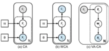
Fig. 1. Graphical representations of augmented (solid boxes) and regular (dashed boxes) mixture models for a set of N independent and identically dis-tributed (iid) data samples. Random variables depicted in circles, transparent for latent variables, shaded for observed variables and stripping for variables that can be observed or latent on occasion. Model parameters are illustrated with squares.xiare the observed data samples,zithe latent class labels and
cithe contextual variables. Model (a) gives rise toCA–type of estimation and (b) toWCA. Model (c) depicts the graph of a variational autoencoder-based mixture for the equivalent ofCAestimation.
The proposed idea is best explained in the framework of FMMs, the simplest and most basic Bayesian network. In order to gain a solid understanding, the reader should recall [3, chap. 9.2] that a FMM is represented by the direfted graph illustrated in Fig. 1a-b (enclosed in a dashed box), where xi ∈ X is the observed independent and identically
distributed (iid) data samples of a dataset X with cardinality N (i ∈ [1, N]), zi ∈ Z is the latent data representing the
mixture/class generating sample xi having a 1–of–M
repre-sentation, so thatzij ∈ {0,1},Pjzij = 1andM the number
of mixtures/classes. The distribution of observed dataxis then p(x) =P zp(x,z) = P zp(z)p(x|z) = PM j=1πjfj(x,θj),
where, πj = p(zj = 1) are the mixture coefficients with
PM
j=1πj= 1 andf(x,θ0) =p(x|z,θ0)withf belonging to
some identifiable family with parameters θ0. ML estimation consists in maximizing the logarithm of the incomplete– data, marginal likelihoodlogL(θ|X) =log(QN
i=1p(xi))over
θ. In supervised estimation, zi are the observed labels yi,
yielding analytic solutions. Conversely, for latentzione relies
on the iterative EM–MLE, where, first, the expectation (un-der posteriorsp(z|x,θ)) of the complete–data log–likelihood logLc(θ|X, Z)is formed (E–step):
Q(θ,θˆk) =Eθˆk{logLc(θ|X, Z)}= N,M X i,j Eθˆk{zij}logπj+ N,M X i,j Eθˆk{zij}log(fj(xi,θj)) (1)
whereθ ={πj,θj},∀j are the overall estimated parameters
andθˆk the kth estimate. Then,Q(θ,θˆk) can be analytically maximized (M–step):θˆk+1= argmax
θ
{Q(θ,θˆk)}.
This conventional unsupervised EM–MLE algorithm (termed hereafterUS) is known to get stack in local maxima (thus being sensitive to the initialization θˆ0) and exhibits compromised estimation precision compared to supervised estimation (termed S). Furthermore, it is inferior to S in terms of standard errors and convergence rate (since it is iterative). It is clear that these limitations should be related to the missing label information. Both methods share the same objective of (1), only differing in the replacement of labelsyi
(S) by posteriorsEθˆk{zij}=p(zi =j|xi,θˆk)(US). Hence,
it is reasonable to assume that boosting the information content (entropy) of distributionsEθˆk{zij}towards the labels
yi should raiseUS performances closer to those ofS.
The idea put forward in this article is to achieve this goal by directly embedding probabilistic side–information into a generative model. More specifically, it suffices that a) con-textual information can be modeled by (in general, latent) random variablesci2 which b) can be assumed to have a
de-pendence relationship with the latent nodeszi(augmenting the
underlying model, as shown in Fig. 1 for the case of FMMs) and c) whose distributions p(ci) and/or p(zi|ci), p(ci|zi)
are known. Given these prerequisites, deriving context-aware algorithms results from straightforward application of MLE on the augmented models, which results in the regular EM algorithm for FMMs. Analytical derivations can be found in Appendix B.
It is critical to discuss what these assumptions imply for the applicability of the proposed approach. The first prerequisite is a mere modeling choice and hardly restrictive, since all natural quantities can be modeled as random variables. The second assumption forms the basis of our framework. It advocates for a paradigm shift where one needs not solely rely on the possibility to collect usual “data and labels”, but can instead identify contextual sources of information that may partially reveal the missing data labels. Of course, this might not always be possible. The third assumption can also be limiting since, even after identifying potentially useful types of context, the distributions p(c), p(z|c), p(c|z)could still be unknown, difficult to pre-estimate, or rather uninformative. For instance, in the medical informatics example used in Section I, medical tests additional to X-ray imaging for lung tumour detection might be as hard, expensive or dangerous 2Without loss of generality, the contextual random variables will be
to collect as the biopsy that would reveal the actual ground truth labels (malignant or benign). In addition to this, this last prerequisite can only be satisfied for fully definedz (i.e., known number of mixtures M), which limits the scope to unsupervised classification. Hence, with respect to the last two assumptions, there can be no guarantees of existence or benefits, or even a way to analytically quantify the likelihood of those in general applications. Nevertheless, in the era of information explosion and the emergence of the Internet Of Things, we believe that these assumptions can be already satisfied more often than not, with the situation improving in the foreseeable future.
The two possible types of dependence between ci and zi
give rise to two different augmented models (Fig. 1a and b) and, therefore, two corresponding EM–MLE algorithms termed CA and WCA, respectively. We are also considering a third, heuristic algorithm termed DCA (Direct Context– Aware), where the posterior distribution of latent labels is defined by arbitrary probabilistic labels and the evidence X is ignored. Table I summarizes the naming convention, probabilistic labels pi, E–step andlogL formulation of each
algorithm.
From a factor graph perspective [3, chap. 8.4.3], the basic premise of CAandWCAis the provision of additional (com-pared to US) information through the messages passed to the latent nodeszi. As evident in the E–steps of Table I,USonly
benefits from evidence X, while belief propagation with CA and WCA should be richer due to the additional contextual variablesC. Of note, in the originalS/USestimation problem θ is not cumbered with additional parameters related to the contextual variables, despite the model augmentation, due to the assumption of known priors and conditionals. It follows that the graphical representation of contextual assistance can be more complex than a single variable c, as long as the conditions of no additional parameters and seamless message parsing are satisfied. Essentially, the need for ground truth is replaced by a lesser requirement for knowledge of the aforementioned distributions. Those can be learned prior to the deployment of the algorithms, or even be publicly available (e.g., language models).
As already illustrated (Table I), the context–related terms of each algorithm can be isolated to implicitly define sample-wise probabilistic “labels” pij withPMj=1pij = 1 (i.e., each
piis a discrete probability distribution over the latent variable
zi). The entropy of these labels represents a measure of the
contextual information content individually for each sample xi and, by averaging, for the overall estimation problem. Our
work is the only one, besides [40], highlighting the impor-tance of side–information measurability for the prediction of estimation benefits, our primary axis of investigation.
B. Information matrices and missing information principle In order to shed light on the fundamental issue of alleviating the missing label information through the provision of side– information, one can rely on the Fisher Information [44], the most formal way of measuring the amount of information involved in the estimation of the unknown parameters θ.
Therefore, we study approximations of the (expected) Fisher information matrix I(θ) through its sampled-based version, theobserved information matrixI(θ|X). The latter measures the amount of information a sampleXcarries on the estimated parameters θ, where I(θ) = Eθˆ[I(θ|X)] and I(θ|X) =
−∂logL∂θ∂θ(Tθ)|θ=θˆM L, the negative of the Hessian of the log-likelihood objective function evaluated at the ML estimate.
In [7], it is proved that the observed information for missing–data problems can be computed as the difference I(θ|X) = Ic(θ|X) −Im(θ|X). The first term is an
es-timate of the available information if there were no miss-ing data. The second term, called the missmiss-ing information matrix, represents the information lost due to missing data. This relation has been called the missing information prin-ciple (MIP). Both these matrices can be computed through complete–data quantities (so that their calculation is tractable), as: Ic(θ|X) = Eθˆ{−∂
2logLc
∂θ∂θT }|θ=θˆM L and Im(θ|X) =
covθˆ{Sc(X|θ)Sc(X|θ)T}|θ=θˆ
M L, where Sc(X|θ) is the
score (gradient vector) of the complete–data log-likelihood. The Fisher information also allows for the computation of the variance–covariance matrix of the MLE, asC=I−1(θ|X)
and, hence, the standard errors of parameter estimation as SEi= 2
q
Ii,i−1(θ|X)for theithparameter in vectorθ, without
resorting to repeated sampling. The same is true for the algo-rithms’ convergence rate, since, when EM converges to a local maximum, it has been shown [45] that the convergence rate r= limk→∞k
ˆ
θk+1−θˆk
ˆ
θk−θˆk−1kis linear and coincides with the
spec-tral radius (λmax, whereλi∈[0,1),∀i, the eigenvalues) of the
“rate” matrix J, defined asJ(θ) =I−1
c (X|θ)Im(X|θ). The
latter expresses the total fraction of missing information [46]. In Section IV we use the definitionr0 = 1−r= 1−λmax,
which complies with the intuition that0 corresponds to non-converging and1 to immediately converging algorithms. C. Likelihood landscapes
Fig. 2a illustrates the incomplete–data log–likelihoods logL(µ1) and the intermediate objectives maximized at the first M–step (complete–data log–likelihood expectations plus the latent data entropy) Q(µ1,µˆ10) +H( ˆµ10,µˆ10) (see Ap-pendix B) for a mixture of two univariate Gaussians3. The
estimation precision benefits of context–aware algorithms (in case of “correct” context as in the example) come as a result of a favourably modified logL(θ) (compared to that ofUS). These log–likelihoods (here with N E = 0.7) tend to have a larger local maximum close to the supervised estimate (black ‘x’) and, hence, also closer to the true parameter value. This maximum will thus also tend to be the global maximum. Even more, the other local maxima are suppressed, reducing the sensitivity to initialization (where US is known to perform poorly). In Fig. 2a, all context–aware algorithms “escape” (in contrast toUS) the local maximum ofUSon the right side of
ˆ
µ10 and converge to the first local maximum on the left side
3Onlyµ
1is estimated starting fromµˆ10= 2. Parametersπ1= 0.1, µ2=
1, s1 = 0.5, s2 = 3are fixed. Estimation is based onN = 100randomly
generated samples withµ1= 0. This setting is selected among those leading
to multiple local maxima, so that the effects of the proposed algorithms can be clearly illustrated.
TABLE I
ALGORITHMS UNDER STUDY.US: REGULAR UNSUPERVISEDEM–LEARNING.CA: CONTEXT–AWAREEM–LEARNING.WCA: WEIGHTED
CONTEXT–AWAREEM–LEARNING.DCA: DIRECT CONTEXT–AWARE LEARNING.S: REGULAR SUPERVISED LEARNING.
pi E–step Eθˆ{zij}=. . . logL= N P i=1 log( M P j=1 (. . .)) US None πjfj(xi|θˆj) M P m=1 πmfm(xi|θˆm) πjfj(xi|θˆ) CA P ci p(ci)p(zi|ci), latent C p(zi|ci), observed C pijfj(xi|θˆj) M P m=1 pimfm(xi|θˆm) pijfj(xi|θˆ) WCA p(ci|zi) p(ci) pijπjfj(xi|θˆj) M P m=1 pimπmfm(xi|θˆm) pijπjfj(xi|θˆ) DCA Custom pij πjfj(xi|θˆ) S yi ( 1 , yi =j 0 , yi 6=j πjfj(xi|θˆ)
(‘x’ of the respective color). The latter is much closer to the true parameter value, yielding higher estimation precision.
The magnitude of these effects increases with increasing contextual negentropyN E, as shown in Fig. 2b. AsN E→1
(dotted lines) the problem reduces to supervised learning. Furthermore, in the case of ignorant context (N E = 0), the WCA objective (solid green line) reduces to a translated version of that of US(red), while CA(blue) already “boosts” the favorable maximum. Hence, for “ignorant” context,WCA is identical to US, while CA can already yield improvements in precision.
The improvement of convergence rate and its dependence on contextual negentropy are also implied in the example, since the estimates µˆ1
1 (first iteration) for CA (blue ‘o’) and WCA (green ‘o’) are much closer to their final MLE than for US (red) or CAE (CA with ignorant context, magenta). This fact is further substantiated in the next section. DCA, as elaborated later, underperforms in comparison to the other context–aware algorithms, suggesting that discarding data– dependent evidence completely is suboptimal.
D. Standard errors and convergence rate through the MIP The application of the missing information principle (MIP) on algorithms CA, WCA and US is demonstrated in a (ran-domly selected) mixture of two univariate Gaussians problem4.
For each (increasing) N E value, we perform 100 repetitions randomly generating N = 104 samples from the above distribution and estimate the algorithms’ average (across rep-etitions) standard errors and convergence rates.
For one repetition of the aforementioned problem, Fig. 2c (for WCA) and 2d (forCA) show that matrices Ic (first row)
remain unaffected by increasingN E, since the complete–data information Ic = IS should be independent of any side–
information. On the contrary, the magnitudes of the elements of the missing information matrix Im (second row), which
4π
1= 0.6, µ1= 0, µ2= 1, s1= 1, s2= 2. Parameterss1,s2 are fixed. π1, µ1, µ2are estimated from initialπˆ10= 0.5,µˆ10= 0.49,µˆ20= 0.51.
for N E = 0 obtains its maximum IM AX
m =ImU S (when no
additional information on missing labels exists), are reduced with increasing N E, to eventually vanish into the 0 matrix as N E → 1 (ImM IN = ImS = 0, since data labels are fully revealed by context). Consequently, the fractions of missing information (rate matrix J = Ic−1 ∗ Im, third row) also
vanish, along with its spectral radius. Hence, the missing label information in context–aware EM learning is shown to be eliminated proportionally to the information content of the provided side–information.
The finally available information in these algorithms, as encoded in the information matrices I = Ic − Im (MIP
definition), will consequently be bounded. Above, byIM AX =
IcM AX −ImM IN = IcS −0 = IS (identical to the super-vised MLE, S) and below by, IM IN = IcM IN −ImM AX =
IcS−ImU S = IU S (identical to the unsupervised MLE,US).
Expressions IcM AX = IcM IN = IS and ImM AX = ImU S and
IM IN
m =ImS = 0hold by definitions. These exemplary results
are substantiated and shown to generalize to arbitrary FMM problems by Propositions 1–3 of Appendix D.
Fig. 2e illustrates the average predicted standard errors of estimatesπˆ1 (♦),µˆ1 (O) andµˆ2 () as well as their sum (◦) with increasing contextual negentropy N E for US (red),CA (blue) andWCA(green). Indeed, it is illustrated that standard errors of all parameters (see below for the explanation of exceptions), as well as their sum, decrease with increasingN E for bothCAandWCA, converging towards the corresponding standard errors of S at N E = 1. Similarly, Fig. 2f shows that the convergence rate r0 of CA (blue) and WCA (green) is improved with increasing N E to reach single–iteration convergence (r0 = 1, likeS) in the case of “perfect” context (N E = 1). Thus, as expected (Section III-B), stronger side– information improves the performances on these two metrics. Interestingly, the standard errors and convergence rates of CA are superior to theirWCAequivalents for the wholeN E spectrum, until both algorithms converge to their S limit at N E → 1. CA thus yields a better lower bound than the regularUSperformances, exhibited byWCA. This is due to the
(b) (a) (c) WCA μ1 μ2 π1 μ1μ2π1 (d) CA μ1 μ2 μ1 μ2 +1 -1 0 (e) Contextual Negentropy, NE A ver age Stand ard Er ror s (f) Contextual Negentropy, NE A ver age Conve rgence Rate
Fig. 2. (a)logL(µ1)(solid lines) andQ(µ1,µˆ10) +H( ˆµ10,µˆ10)(at first EM iteration, dashed lines) for various estimation algorithms as color–coded in the
legend, in a mixture of two univariate Gaussians model.CAErefers to algorithmCAwith ignorant context andCA,WCAandDCAare shown for contextual negentropy N E = 0.7. ML estimates after convergence shown with ‘x’ and estimates after the first iteration in ‘o’. (b) Incomplete–data log–likelihoods
logL(µ1)in the same problem as in (a) forUS(red solid) and various contextual negentropy levels as shown in the legend forCA(blue) andWCA(green).
Information matricesIc,Imand rate matrixJ=Ic−1∗Imwith increasing contextual negentropyN Ein a mixture of two univariate Gaussians estimation problem (see text), for (c)WCAand (d)CA. All matrix values normalized to[−1,1]by dividing with the respective absolute value of theUSalgorithm. (e) Average predicted standard errors ofπˆ1(♦),µˆ1 (O) andµˆ2() and their sum (◦) with increasing contextual negentropyN Ein 100 repetitions of a mixture
of two univariate Gaussians estimation problem. Different algorithms color–coded in the legend. (f) Average predicted convergence rates and their standard deviations for the three algorithms (color–coded in the legend) in the same estimation problem.
structure of the information matrices forCAwhich, compared to those of US/WCA, are reduced by removing the elements associated to the mixing coefficients πj,∀j (as in Fig. 2d).
Essentially, in CA, the mixing coefficient distribution π is independent of X and fully determined by C. The mixing coefficientsπj are computed here forCA as πj = N1 Pip0ij,
where p0ij = 1 if j = argmaxk{pik} and 0 otherwise, an
unbiased estimator exhibiting the same standard errors forπj
as S (“correct” context). The fraction of missing information is always reduced for CA, due to the absence of uncertainty regardingπ5. The lower bound ofCAstill corresponds to that
of US, but the one with fixedπ.
It is also interesting that, exceptionally, the standard errors ofµ1(Fig. 2e) are superior (smaller) forWCArather thanCA. Such exceptions can occur because the missing information is not distributed uniformly across the estimated parameters, or identically among the different algorithms. However, the sum/average of standard errors only depend on the overall fraction of missing information (λmaxofJ), shown to always
reduce with increasing N E (Proposition 2, Appendix D) and be smaller for CA compared toWCA. Furthermore, since the rates of convergence coincide to a global rate only depending on λmax (except for rare cases [48]), the rate of convergence
ofCAis also guaranteed to be greater/equal to that ofUSand WCA(for a given N E).
E. Context–aware learning algorithms for VAs
Formulating the proposed algorithms for other Bayesian networks follows the exact same steps. For example, context-aware learning of Hidden Markov Model (HMM) parameters would exploit contextual variables co-dependent to the hid-den state (with known statistics) and result in a version of the Baum-Welch algorithm with modified E–step to include 5In general, it can be shown by applying Theorem 4 in [47] that removing
any parameter from the estimation problem can only reduce the spectral radius of the rate matrixJ.
side–information, and identical M–step. However, in view of classification tasks, it would be ideal to be able to apply the proposed approach in the context of deep learning with ANNs, which have shown to excel in this task when big data is present thanks to far superior expressiveness than FMMs or other probabilistic generative models. This possibility would also alleviate a major weakness of this literature, namely, the heavy reliance on supervised learning which, alongside the need for (labeled) big data, limits their wider deployment.
At first, this endeavor may seem odd, with several reasons ostensibly preventing the derivation of equivalent context-aware algorithms in this framework. First, contextual random variables cannot be intuitively embedded into non-probabilistic models like ANNs. Most importantly, these are discriminative models conventionally requiring loss functions other than MLE, which demand explicit labels (“targets”). Furthermore, by avoiding to model the data and joint distributions, they yield no regular unsupervised learning algorithm to build upon. Yet, by imposing softmax output layers, ANNs can in fact represent conditional distributions and be trained with MLE. In addition to this, generative deep neural networks admitting probabilistic graphical representations have been recently formulated, the most popular of which is termed variational autoencoder (VA) [4].
Hence, the basic idea is to derive a mixture model with VAs and proceed thereafter to embed context in the exact same way as with the FMMs. Luckily, VAs, as originally proposed [4], already respect the same simple directed graph enclosed in dashed lines in Fig. 1a-b. However, priorsp(z)in this case are Gaussian, so that variableszcannot represent the latent class labels as we would like. It is for this reason that VAs are primarily used for dimensionality reduction–finding a compressed, informative embeddingz of the datax, but are not ideal for clustering purposes. Modeling z as a discrete latent variable to get exactly the FMM graph equivalent is ill-posed, because it prevents the use of the “reparametrization
trick”, which allows gradients to flow through random vari-ables for parameter estimation. Although solutions have been proposed [49], it is simpler to maintain the lower-dimensional embedding, here denoted w, and let it be governed by the latent class labels z as shown in Fig. 1c. This remains more intuitive than other approaches to implement mixture models with VAs (e.g. [50], [51]), many of which assume a Gaussian mixture for the priorp(w), instead. The mixture model in our case is thus defined with respect to the embedding w rather than the datax, an idea introduced in [52] for semi-supervised learning (M2 model). The additional contextual variables are then linked to z as in the FMM case.
The profound similarity of this model’s joint distribution to that of the FMMs (the only difference being the interleaving of w in the message passing between z and x) and the fact that context is embedded in the exact same place and manner, makes it easy to prove that the definitions of probabilistic labels pi are identical to the FMM case (see Appendix B).
The inference model of the context-free case is q(z, w|x) =
q(z|x)q(w|x, z) (where q(w|x, z) the VA’s encoder model), so that the context-enabled version simply consists in fusing probabilistic labelspiwith the distributionq(zi|xi)(softmax
layer output of the corresponding network) for each sample xi, equivalently to the way shown in Table I for p(zi|xi)in
the FMM scenario (the E–step of the EM algorithm). Of note, although in Fig. 1c the CA case for VAs is illustrated, the WCA equivalent can be similarly derived.
Finally, the parameters of all networks defining the mixture-VA (q(z|x)orq(z|x, c), encoderq(w|x, z), decoderq(x|w, z)) are learned with gradient descent. The objective consists of the regular reconstruction loss and the regularization term for priorsp(w), in addition to the variational lower bound that can be written Eq(z,w|x)[log
p(z)
q(z|x)+ log
p(w|z)
q(w|x,z)+ logp(x|z, w)]. It must be underlined that the method is agnostic to the type of ANNs used to implement the graph.
F. Evaluation metrics
The results of Section IV compare five algorithms (CA, WCA, DCA, US, S) in simulations with artificial FMM datasets, as well as in real–world problems. The estimation properties reported are precision, standard errors and con-vergence rate. Estimation precision is the Euclidean distance between the estimated parameter vector θˆand the actual one θA, namely: D=kθˆ−θAk. For standard errors we employ
the aforementioned estimatorSEi. For brevity, we only report
the average ASE = L1PL
i=1SEi (where L is the number
of estimated parameters). Similarly, the MIP–based estimate r0= 1−ris used for the convergence rate. The classification performance of trained models is assessed through N-class accuracy A = Nc/N, where Nc the number of correctly
classified samples out of N total samples across all classes. Finally, for regression tasks, the mean square error M SE is reported.
In order to quantify the information content of side– information, we employ a scaled negentropy definition on probabilistic labels pi: N Ei = 1 +P
M
j=1pijlogMpij. This
metric is conveniently bounded, N Ei ∈ [0,1], for any
number of mixtures M. N Ei = 0 when pi is uniform,
pij = 1/M,∀j ∈ [1, M] (“ignorant” context, pi does not
cast a preference over any class). Conversely,N Ei= 1when
pim = 1, m ∈ [1, M] and pij = 0,∀j 6= m, j ∈ [1, M]
(“perfect” context, fully revealing the class labelyi. TheN E
level of a dataset is extracted as the average across all included labelspi.
G. Simulation design
For our simulation studies, a labelpifor each samplexi is
constructed randomly, so that its information content isN Ei.
For all but one examined scenarios, all samples in X are assigned the sameN Evalue (N Ei =N E,∀i). In the “mixed”
context scenario, however, eachN Eiis randomly drawn from
a fixed interval. In all but the “wrong” context scenario (see below), pi-s are constructed to cast greater confidence to
the ground-truth label yi (“correct” context). Formally, we
impose arg max{pi} = arg max{yi}, so that pi-s always
“predict” the correct yi with increasing confidence as N E
increases. This rule is only abandoned in the “wrong” context scenario, where the effects of misleading contextual informa-tion are investigated. In this scenario, ki = arg max{pi} 6=
arg max{yi}, ki ∈ [1, M]∀i is selected randomly out of the
M−1remaining possibilities for a reported percentage of the generatedpi-s.
The following scenarios are considered with “correct” con-text. A: a mixture of two univariate normal distributions, where variances are known and only the two class means are estimated, B: a mixture of two univariate normal distributions, where all existing parameters are estimated, C: a mixture of three univariate normal distributions, D: a mixture of two multivariate (2D) normal distributions, E: a mixture of two univariate Maxwell–Boltzmann distributions and F: a mixture of two univariate, first order, linear regressors. These six scenarios are chosen to differ in terms of the numbers and types of mixtures employed (where, the Maxwell–Boltzmann of Scenario E is not a member of the exponential family), the number of estimated parameters, the dimension of the input space and the utility of the FMM (classification versus regres-sion). The scenarios targeting “mixed” and “wrong” context situations (Appendix E) employ mixtures of two univariate normal distributions.
For each scenario, 1000 estimation problems are gener-ated and solved for all compared algorithms. Each prob-lem r ∈ [1,1000] is associated to a randomly generated dataset Xr, Yr, PrN E of observed data, ground–truth labels
and probabilistic labels of N E, respectively. For algorithms CA, WCA and DCA, each problem r is further solved for N E ∈ [0 : 0.1 : 0.99], so that our evaluation encompasses the complete range of possible contextual information content. The cardinality N of each dataset is fixed to 100 times the number of parameters to be estimated. The ground–truth Yr is constructed to have balanced number of samples per
class. The observed data Xr are randomly generated from
semi-randomly selected “actual” distributions with parameters θrA (of the respective scenario’s type) and the estimation begins with semi-randomly chosen initializationθˆ0
to all algorithms). These semi-random procedures, detailed in Appendix C, ensure balanced number of samples per class and minimal impact of separability and initialization on the extracted results. All algorithms are left to perform as many iterations t, as needed so that kθˆt
r −θˆ
t−1
r k <10
−5. If this stopping criterion is not reached after 300 iterations for some algorithm, θˆ300
r is used as its final estimate.
The classification accuracyAis computed for each scenario, problem r and algorithm, by generating a second “testing” dataset Xr0, Yr0 (of equal cardinality to Xr) from the same
“actual” FMM, which is classified using the estimated pa-rameters of each algorithm by means of the Maximum–A– Posteriori rule. For the mixture–of–regressions scenario, the same evaluation methodology is applied to derive the M SE on the testing set.
IV. RESULTS
A. Results with artificial data
Sections III-C and III-D justify theoretically the estimation benefits brought forward by the proposed approach. More specifically, in Section III-C we show, on the one hand, how the log-likelihood objectives in this methodology, compared to the US equivalent, exhibit lower local maxima except for the one closer to the supervised estimate. This effect increases the chances of convergence to this favourable extremum by reducing the EM algorithm’s sensitivity to initialization. On the other hand, Section III-D shows that the fraction of missing information of an estimation problem, as expressed by the spectral radius of the rate matrix (see Section III-B), is shown to decrease proportionally to the information content of the provided side–information, bounded byUS andS (maximum and zero missing information, respectively). Therefore, the estimation properties that depend on the fraction of missing information, namely, the standard errors and the convergence rate, also benefit from context–awareness. Appendix D for-mally proves that these effects generalize to all FMMs. The theoretically anticipated effects are verified by simulations with artificially generated data, presented in this section.
The following set of simulations is meant to compare the performances of the derived algorithms for the “correct” context situation. Within each scenario, we illustrate each metric’s average across all 1000 problems for algorithm α and someN E,MN Eα , normalized to be bounded bySandUS performances, as: MfαN E = (M
N E
α −MU S)/(MS−MU S).
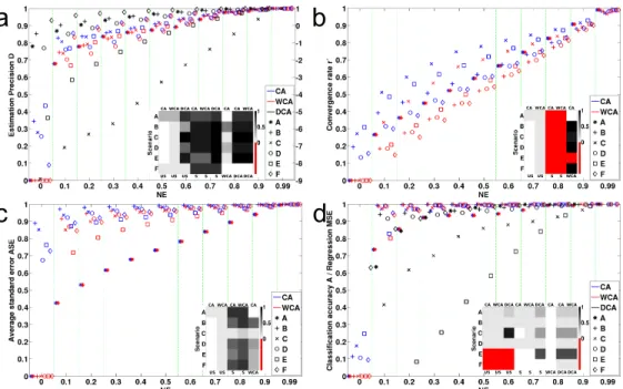
Fig. 3a–b show that, for all examined properties, CA and WCA exhibit improved performances proportionally to the strength of contextual assistance. Additionally, the average performances are upper–bounded by S (at N E → 1) and lower–bounded by US (at N E → 0). CA is consistently outperforming WCAfor the sameN E, while both algorithms yield substantially better D, A and/or M SE than DCA. While WCA reduces to US for N E = 0 (Appendix B and Section III-D), CA yields improvements over US even in this case. Scenario A is an exception occurring for fixed π (Section III-D). These trends are universal, although the magnitude of improvements as a function of N E is metric–
and scenario–dependent, confirming the generalizability of the examples in Appendices III-C and III-D.
Statistical testing reveals that the added value of CA and WCA over conventional unsupervised estimation US is sig-nificant for all metrics, already at very low N E (for CA, even for ignorant context). Scenarios E and F for metrics A and M SE, respectively, are exceptions where improved estimation precision D does not translate into significantly better classification/regression, as an intrinsic property of the respective FMMs. Nevertheless, for metrics D and ASE, it is only at very high N E that CA and WCA become indistinguishably similar toS, while forr0supervised learning S is significantly better even at N E= 0.99. The undesirable significance notwithstanding, the average differences for all metrics tend to operate much closer to the S rather than the US“extremity” even at lowN E(especially forCA). Further-more, concerningAandM SE, context–aware algorithms are statistically similar toSsince very lowN E. The superiority of CAoverWCAis shown to be significant only for the first few tested N E levels for metrics D, ASE and A/M SE, while it persists for almost the entirety of the N E spectrum forr0. Finally,DCAis again shown to underperform.
Last but not least, our simulations demonstrate that context– awareness can substantially reduce the number of problems that could not converge with regularUStraining6. In the most
characteristic example (due to the larger number of mixtures) of scenario C, where 83.7% of problems did not converge withUS, this percentage is reduced byCAto3.8% atN E= 0 and 1.0% for N E ∈ [0.1,0.99]. WCA also alleviates this problem (less aggressively), by gradually reducing the non-convergence percentage to67% atN E= 0.1,39.4% atN E= 0.5and, eventually,1.0% atN E= 0.99. It is thus shown that context–awareness is able to avoid irregularities, already at low N Elevels. In the interest of space, results on more “realistic” situations where contextual assistance can be, to some extent, “wrong” and of “mixed”N E are offered in Appendix E. B. Results on real–world scenarios
1) Gaussian Mixture Models: The versatility of CA and WCAparameter estimation is shown in three different unsuper-vised classification scenarios using Gaussian Mixture Models (GMMs): i) A brain-computer interface (BCI) speller, where the BCI classifier translating brain signals into text-entry actions is learned on-the-fly with CA context derived from a language model and the speller’s structure. ii) Unsupervised CA and WCAtraining of classifiers diagnosing malignancies in mammograms, where known risk factors and manual as-sessments represent the side–information at hand. iii) Unsu-pervised recalibration of fingerspelling classifiers recognizing sign language from video frames, where, again, a language model provides contextual assistance. Detailed methods and results on all these applications are elaborated in Appendix F, while Table II summarizes the average improvements obtained with the proposed algorithms against US, and how their performance compares to supervised learning S. Overall, the 6An EM algorithm fails to converge to a local maximum when the spectral
a
b
c
d
WCA
CA DCACAWCADCA CA CA WCA
USUSUS S S S WCA DCA DCA
WCA
CA DCACAWCADCA CA CA WCA
USUSUS S S S WCA DCA DCA WCA CA CAWCACA US US SS WCA WCA CA CAWCACA US US S S WCA
Fig. 3. Normalized, average (across 1000 problems of each of 6 FMM estimation scenarios A–F): (a) estimation precisionD(right y-axis only refers toDCA performances), (b) convergence rater0, (c) average (across parameters) standard errorASEand (d) classification accuracyA/regression mean square error
M SE. The performances of each context–aware algorithm (CA,WCA,DCA) for each scenario A–F are color– and shape–coded as shown in the legends. Performances for differentN Elevels arranged along the horizontal axis. For each metric and scenario, the embedded colormaps illustrate the lowest (when USis involved) or highest (for all other combinations)N Elevel (color–coded as shown in the adjacent colorbars) above which the algorithms on top and bottom of each column significantly differ at the 95% confidence interval (one–sided, paired Wilcoxon rank–sum tests with Bonferroni correction for multiple comparisons). Red color denotes no significant difference for anyN Elevel.
TABLE II
CONCENTRATED CLASSIFICATION ACCURACY RESULTS(%)FORFMM
UNSUPERVISED CLASSIFICATION APPLICATION SCENARIOS: (A) BCI, (B)
CANCER DETECTION AND(C) FINGERSPELLING.
US CA WCA S
A 52.4±8.1 64.7±6.5 - 66.2±7.2
B 79.6±8.5 88.1±3.4 89.8±3.1 91.8±1.9
C 61.0±9.4 72.1±7.9 - 90.1±2.9
findings of the simulations with artificial data are shown to replicate with realistic data, the main conclusion being that the proposed context-aware learning significantly outperforms reg-ular unsupervised learning in terms of classification accuracy, and is competitive to the supervised case in spite of discarding the need for ground truth labels.
2) Variational autoencoders and comparison with a neural-symbolic method: The applicability of the idea put forward in this paper with generative deep neural nets is shown by employing the VA-based mixture model explained in Sec-tion III-E to perform unsupervised classificaSec-tion of the well-known MNIST benchmark database of handwritten digits (55000 training and 10000 testing labeled samples for 10 classes–digits 0 to 9). Since our goal is to show the merits of context-aware learning and not to optimize the network architecture, we vectorize the 28x28 pixel images (to 784-dimensional input vectors) and use regular, non-convolutional layers. Specifically, the encoder model consists of 2 hidden layers with 512 units each, and an additional third layer with
128 units (64 + 64) to output the means and variances of the latent space w. The decoder model consists of 3 layers with 512, 512 and 784 units, while the modelq(z|x)contains 3 layers with 512, 512 and 10 units. RelU activation is used everywhere apart from the output layers of the decoder (logit), the q(z|x) network (logit+softmax) and the encoder (no activation for means and softplus for variances, to imitate a covariance matrix).
Contextual information derives by considering a scenario of (numerical) student ID recognition as part of an automatic exam paper processing system. Due to the inherent structure of such identification systems (e.g. serial historical number-ing, continuity within a university department), the place of a digit within the student ID reveals a lot of information about its potential identity, while the statistics of this kind of side–information can be very easily acquired through the university’s database (importantly, with view to such use, reg-istrations can be manipulated to yield even richer information content). Specifically, we assume a realistic case of 5-digit-long IDs, where the first digit is always 1, the second is 7/8/9 with probabilities 0.05/0.80/0.15, respectively, and the remaining three places yield distributions that slightly diverge from the uniform one, each favouring some of the remaining digits. For our simulations, we generate randomly such student IDs and assign MNIST samples and probabilistic labels pi
accordingly to each digit.
We compare this approach with the algorithm proposed in [42], which we consider to be the most relevant work in the ANN literature for learning with side–information. This method distills additional information in the form of logic rules (hence its affinity to neural-symbolic integration). Its
basic premise is an iterative knowledge distillation algorithm, which augments the objective function of a regular supervised ANN with an extra term encouraging the network’s softmax output to fit, in addition to the ground truth labels y, also a “soft” prediction s. The latter results from the fusion of the network’s output with evidence from the logic rules (Eq. 4
in [42], what the authors call the “teacher network” output). Of note, since rules are ultimately used to constrain p(z|x), the authors admit that, like we have also denoted for our own algorithms (Appendix A), this method also falls under the class of Posterior Regularization.
For a fair comparison based on the same model and type/level of contextual assistance, we employ the same ANN q(z|x) that is part of our VA–based mixture formulation and set the soft prediction s to be the Bayesian fusion of the same probabilistic labels pi, with the network’s output
q(z|x) (i.e., the two distributions are multiplied and the result is normalized). Since this method explicitly balances the supervised and the rule-based objectives with a regularizer π∈[0,1](Eq. 2), we compare with: i)Sd:π= 0, i.e., regular supervised training of the discriminative model, ii) Knowledge distillation (KD) KD0.1: π = 0.1, iii) KD0.5, iv) KD0.9, v) KD1.0 (pi= 1.0, thus ground truth labels are ignored and the network is trained only on side–information) and vi) KDexp: πt= 1−0.95t, wheretthe epoch. These are compared to
VA-US (the softmax outputq(z|x)of our model is left untouched by context),VA-CAandVA-S(class labels are fed as contextual assistance). A limited number of labeled data (only 10 per class) are used to “seed”VA-CAso as to enforce theithcluster
to represent the corresponding class (otherwise it is unknown in what order the elements of probabilistic labels pi should
be presented to the algorithm), while the same data are used to associate the found clusters to the digit classes for VA-US (the class with most such samples in a cluster “wins” it).
We run ten repetitions of the learning problem (100 epochs) with each algorithm (exceptionally, 30 repetitions for VA-CA) and record the finally convergent classification accuracy of each repetition. We obtain the following results, VA-US:
71.0±9.0,VA-CA:82.2.0±15.4,VA-S:98.1±0.07,Sd/KD0.0:
98.1±0.09,KDexp:49.5±0.1,KD0.1:98.2±0.06,KD0.5:
97.9±0.06, KD0.9: 86.3±0.2, KD1.0: 49.3±0.05. First, it is clear that our VA-based context-aware algorithm per-forms equivalently to the simple FMM-based one: it signifi-cantly (p = 0.03 with a non-parametric, two-sided ranksum test) outperforms the corresponding VA-US algorithm and approaches the performance of VA-S. This implies that the basic idea proposed here is applicable to complex, high-dimensional problems, which simple generative models may not be expressive enough to solve, so that deep learning is required. The fact that VA-CA is still inferior to VA-S by a large margin is due to the fact that certain repetitions still get stack to local minima (the best repetitions converge to 96%). Safely assuming that this algorithm has a similar effect on the likelihood landscape as in the FMM case (see Section III-C), stronger context should be able to alleviate this issue. However, we believe that a more expressive ANN (i.e., with more hidden layers and/or convolutional layers) may also be able to cope with this. Another important observation is that, when trained
in an supervised manner, the extra parametrization of the VA-based model is not detrimental to classification accuracy, since this model performs similarly to Sd. Hence, generative models can be equally effective for classification tasks to their discriminative counterparts, while being able to do in parallel much more than that. However, it should be highlighted that this is probably only true when enough data are available, as in this exemplary case.
On the contrary, the same side–information exploited through the knowledge distillation method of [42] does not seem to improve substantially over the regular supervised case (the improvement ofKD0.1overSdis marginal and may also be random due to the small number of repetitions performed here). The hyperparametrizations where substantial importance is given to the side–information–based objective (KDexp, KD0.9, KD1.0) perform poorly, while those where the influ-ence of context is reduced simply converge to the supervised performances (i.e., context seems to have no impact). This was somewhat anticipated, since the weak information provided on the data labels through context seems redundant when strong information of the actual labels is available. Of note, the results in [42] do not question this conclusion, because the benefits demonstrated thereby are also slight and likely attributed to the fact that manual labeling in the cases examined there (i.e., sentiment analysis) are rather ambiguous and noisy (thus, ground truth information is also weak, allowing a margin of improvement through logic rule constraints). This should be considered additionally to the fact that the approach proposed here has anyway the advantage over knowledge distillation of being unsupervised. A final important observation regards the compromised performance of KD1.0. Our FMM-based results suggested that theDCAmethod underperforms (unless very strong contextual assistance is available), which led us to confirm that data evidence carries a lot of information that should not be ignored. Extending this conclusion, since KD1.0 performs much worse thanVA-US, it seems that even if data evidence is employed, this wont be enough if the underlying model is discriminative and does not model the data distribution.
V. DISCUSSION
This work has studied unsupervised MLE algorithms devoid of any need for data labels, but able to exploit side–information in the form of probabilistic context embedded into a generative model and with known statistics. A comparative analysis and in–depth study of these algorithms’ properties for finite mixture models is offered from both a theoretical and a practical standpoint. An implementation with VAs extending the same idea to deep learning is also provided.
We argue that the literature of learning from side– information has largely ignored the merits of such fundamental techniques in favour of alternatives mostly stemming from the theory and practice of undirected graphs, which can often be less practical. As an example, we find that in most application scenarios and for most prospective users, it should be possible and much more intuitive to express a given type of side– information as a random variable with known statistics linking
it to the missing class labels, rather than through a generalized expectation criterion or a “feature expectation”. In other words, the admittedly greater generality and flexibility of PR can be most often traded off (Appendix A). Simplicity of the resulting derivations and formulations can only be viewed as additional advantages. We thus consider bringing this methodology in the spotlight to be the main contribution of this article.
Another contribution entails the identification of basic principles giving rise to improved EM–MLE by context– awareness. First, we have shown that a context–assisted log– likelihood objective is favourably distorted in comparison to the regular one, so that sensitivity to initialization diminishes and the chances of convergence closer to the supervised MLE increase. The second principle regards the partial elimination of missing label information through context as a result of the applicability of the MIP. Demonstrating this makes our work the first one to justify the benefits of side–information in learn-ing from an information–theoretic viewpoint. Through these principles, we have established experimentally and, wherever possible, also formally, two important points. First, that any positive effects on the estimation properties are proportional to the information content of implicitly extracted instance– wise probabilistic labels. Second, that the proposed algorithms perform between the boundaries defined by the unsupervised and supervised equivalents of a given problem.
We have showcased that estimation benefits are still evident and significant in problems with variable, weak, or even, to a certain extent, “wrong” contextual assistance, situations likely to arise in practical applications. Furthermore, the algorithms’ limitations and comparative advantages have been outlined. In this regard, we have demonstrated that completely disregarding the evidence from observed samples in favour of context, like with the DCA algorithm, or attempting to exploit it when the underlying model is not generative, yields inferior estimation properties. A general superiority of CAoverWCA as a result of removing missing information related to the mixing coefficients has also been demonstrated. Furthermore, the application of all algorithms in tough, real–world prob-lems, and extensibility to deep learning scenarios, showcases the broad applicability of context–aware learning as proposed here.
As argued in Section III, the main limitation of the al-gorithms proposed here is their non–universal applicability. However, this is not specific to the proposed framework, but, rather, a limitation shared among all methods exploiting side–information. Indeed, it is not guaranteed that for any application exploitable context as shown here exists, or that the cost of automatically retrieving contextual assistance will be lower than that of explicitly labeling data. However, as the real–world examples of this paper illustrate, rich context should be easily and cheaply acquired in a broad application spectrum. Another limitation regards the fact that the prereq-uisite knowledge of distributionsp(z|c)or p(c|z)implies that the latent class labels are at least defined, i.e., the number and type of mixtures/classes M is known. Consequently, the proposed methodology regards unsupervised classification and not general clustering problems.
ACKNOWLEDGEMENTS
This work was supported by the European ICT Programme Project FP7-224631 and the Hasler Foundation, Switzerland.
REFERENCES
[1] O. Chapelle, B. Sch¨olkopf, and A. Zien, Eds.,Semi-Supervised Learning. Cambridge, MA: MIT Press, 2006.
[2] R. S. Sutton and A. G. Barto,Reinforcement Learning: An Introduction. MIT Press, 1998.
[3] C. M. Bishop,Pattern Recognition and Machine Learning. Secaucus, NJ, USA: Springer-Verlag New York, Inc., 2006.
[4] D. P. Kingma and M. Welling, “Auto-encoding variational bayes,”CoRR, vol. abs/1312.6114, 2014.
[5] G. S. Mann and A. McCallum, “Generalized expectation criteria for semi-supervised learning with weakly labeled data,” J. Mach. Learn. Res., vol. 11, pp. 955–984, 2010.
[6] K. Ganchev, J. Grac¸a, J. Gillenwater, and B. Taskar, “Posterior regu-larization for structured latent variable models,”J. Mach. Learn. Res., vol. 11, pp. 2001–2049, 2010.
[7] T. Orchard and M. A. Woodbury, “A missing information principle: Theory and applications,” inProc. 6th Berkeley Symp. Math. Stat. Prob., 1972, vol. 1, pp. 697–715.
[8] T. Cour, B. Sapp, and B. Taskar, “Learning from partial labels,”J. Mach. Learn. Res., vol. 12, pp. 1501–1536, 2011.
[9] Y.-C. Chen, V. M. Patel, J. K. Pillai, R. Chellappa, and P. J. Phillips, “Dictionary learning from ambiguously labeled data,” in Proc. CVPR IEEE, 2013, pp. 353–360.
[10] Y. Sun, Y. Zhang, and Z. Zhou, “Multi-label learning with weak label,” inProc. 24th AAAI Conf. Artif. Intell., 2010.
[11] P. Zhang and Z. Obradovic, “Learning from inconsistent and unreliable annotators by a Gaussian mixture model and Bayesian information criterion,” inProc. Europ. Conf. Mach. Learn. Knowl. Disc. Databases (ECML PKDD’11) - Volume Part III. Springer Verlag, 2011, pp. 553– 568.
[12] K. Audhkhasi and S. S. Narayanan, “A globally-variant locally-constant model for fusion of labels from multiple diverse experts without using reference labels,”IEEE Trans. Pattern Anal. Mach. Intell., vol. 35, no. 4, pp. 769–783, 2013.
[13] C. Liu and Y.-M. Wang, “TrueLabel + Confusions: A spectrum of probabilistic models in analyzing multiple ratings,” in Proc. 29th Int. Conf. Mach. Learn. (ICML’12). New York, NY, USA: ACM, 2012, pp. 225–232.
[14] C. Ambroise and G. Govaert,EM Algorithm for Partially Known Labels. Berlin, Heidelberg: Springer Berlin Heidelberg, 2000, pp. 161–166. [15] I. Muslea, S. Minton, and C. A. Knoblock, “Active + Semi-supervised
Learning = Robust Multi-View Learning,” inProceedings of the Nine-teenth International Conference on Machine Learning, ser. ICML ’02. San Francisco, CA, USA: Morgan Kaufmann Publishers Inc., 2002, pp. 435–442.
[16] X. Yi, Y. Xu, and C. Zhang, “Multi-view EM Algorithm for Finite Mixture Models,” inPattern Recognition and Data Mining, Third Inter-national Conference on Advances in Pattern Recognition, ser. ICAPR 2005, vol. 3686. Berlin, Heidelberg: Springer, 2005.
[17] J. Foulds and P. Smyth, “Multi-instance mixture models and semi-supervised learning,” inProc. SIAM Int. Conf. Data Min., 2011. [18] J. Luo and F. Orabona, “Learning from candidate labeling sets,” inAdv.
Neural Inf. Process Syst. 23, 2010, pp. 1504–1512.
[19] A. Joulin and F. R. Bach, “A convex relaxation for weakly supervised classifiers,” in Proc. 29th Int. Conf. Mach. Learn. (ICML’12). New York, NY, USA: ACM, 2012, pp. 1279–1286.
[20] Q. Nguyen, H. Valizadegan, and M. Hauskrecht, “Learning classification with auxiliary probabilistic information,” inProc. 11th IEEE Int. Conf. Data Min. (ICDM’11), 2011, pp. 477–486.
[21] C. Bouveyron and S. Girard, “Robust supervised classification with mixture models: Learning from data with uncertain labels,” Pattern Recogn., vol. 42, no. 11, pp. 2649–2658, 2009.
[22] E. Szczurek, P. Biecek, J. Tiuryn, and M. Vingron, “Introducing knowl-edge into differential expression analysis,” J. Comput. Biol., vol. 17, no. 8, pp. 953–967, 2010.
[23] Y. Yasui, M. Pepe, L. Hsu, B.-L. Adam, and Z. Feng, “Partially super-vised learning using an EM-boosting algorithm,” Biometrics, vol. 60, no. 1, pp. 199–206, 2004.
[24] R. Urner, S. Ben-David, and O. Shamir, “Learning from weak teachers,” J. Mach. Learn. Res. Proc. Track, vol. 22, pp. 1252–1260, 2012.