Analysis of PID Control Design Methods for a Heated Airow Process

(1)

Helsinki University of Technology

Faculty of Information and Natural Sciences Department of Mathematics and Systems Analysis

Mat-2.4108 Independent research projects in applied mathematics

Analysis of PID Control Design Methods for a Heated Airow Process

April 17, 2008 Tapani Hyvämäki

Instructors: Lic. Tech. Lasse Eriksson M. Sc. Antti Pohjoranta

(2)

1 Introduction

The Department of Automation and Systems Technology is responsible for organizing a laboratory course on automation and control engineering for undergraduate students at the Helsinki University of Technology. One of the fundamental objectives of the course is to cover the basics of PID1_{controllers and} PID controllers' tuning methods. The current laboratory exercise on PID control included in the course has been found to be in need of improvements. The aim of this special assignment is to examine methods to renew and modernize the contents of the laboratory exercise and to give students more illustrative and practical exercise to systems' control.

The case process under study is a heated airow process. It is described more precisely in Section 2. First we introduce the system model and the principles of parameter estimation. Dierent PI and PID control methods and also more complicated control methods as well as the tools for analysis and comparison of the controllers are described. Also, some aspects that have to be taken under consideration when implementing controllers are discussed. After familiarization with the used methods, the parameter estimation, simulations with the model and calculations of performance and robustness are performed. As a result, a thorough analysis of the performance and suitability of the controllers to the case process is performed. Comparison of the methods in the sense of performance and robustness is considered and a short discussion of the results from the educational point of view is included.

The results obtained here are utilized in the development of the laboratory exercise and in its software implementation. However, the nal development and software implementation are not in the scope of this research project though the model implementation and scripts connected to the derivation of the results of this work will be used in the development of the laboratory course material and software.

2 The Case Process

The heated airow process that has been and will be still used as the case process in the laboratory exercise consists of a fan element, heater sink, tube and temperature sensor. The fan produces an airow owing through the tube with constant speed. Air is heated in the beginning of the tube with the heater whose heating power can be adjusted with a control signal. The air temperature is measured with a temperature sensor at dierent distances along the tube. The airow speed inside the tube can be manually controlled by a throttle control. The throttle control angle can be adjusted between 10◦₋₁₇₀◦_{. In this work we use constant throttle control value of}₄₀◦_{. The temperature sensor position}

is also preserved at the distance of 13.4 cm. A schematic illustration of the process is shown in Figure 1. The control signal of the process is bounded to interval 0..10V. It is approximately linearly propor-tional to heater power and can produce a temperature dierence up to 60◦_{C between the inowing and}

(4)

Figure 1: A schematic gure of the case process [9]

out-owing air. The measurement signal is also bounded to interval 0..10V and is linearly proportional to the airow temperature. [9]

2.1 Process Identication

The heated airow process can be modeled starting from heat conducted from heater to owing air and again conducted from air into the temperature sensor. This leads to a linear distributed parameter model of rst order represented in [9]. This model can be simplied into a second order linear process, which has the transfer function

G2(s) = Ts(s) P(s) = K (Tas+ 1)(Tbs+ 1)e −sL2_, (1)

where parametersTa andTbare system time constants,L2is output delay andK is static gain. Output

Tsis the simulated temperature and it is the temperature above the room temperature. From now on we denote the set of these model parameters asP2={K, Ta, Tb, L2}, the subscript 2 referring to the model

order. In the future, we will also denote the system inputP(t)withu(t)and outputTs(s)withy(t). The model presented above does not take into account, for example, little turbulence in the airow or heat conduction from owing air into the tube before the temperature measurement and vice versa. However, these eects can be assumed to be minimal if the system is operating at some small temperature interval, i.e., varying input signal only at some small interval (and keeping the airow speed constant) keeps also the temperature at bounded interval and the heat conduction minimal.

In many cases a rst order approximation of the system is accurate enough to model the process and as will be seen later, many PID tuning methods base on this approximation. Such a system has a transfer function

G1(s) = K

T s+ 1e

−L1s_, (2)

whereT is the time constant,L1is delay andKis the static gain of the system. Later on we will denote

(5)

0 2 4 6 8 10 −0.2 0 0.2 0.4 0.6 0.8 1 1.2 1.4 time y(t) / u(t) 63.2% K₂ T L 1 K 1 K₂

Figure 2: Tangent method for rst order model parameter determination, static gainK=K2/K1.

2.2 Parameter Estimation

In order to obtain proper results when using the system models introduced in previous section, the model parametersP2andP1need to be estimated. For our purposes it is sucient to estimate the parameters

at each operating point at a time or use the same estimated parameters in an operating interval as wide as possible. Estimation of parameters P2 is performed by tting the model output curve to measured

process output values for a step input. The curve is tted using the least squares method. So, we minimize the sum of squares

min P2 E(K, Ta, Tb, L2) = n X k=1 ¡ Tm,k−Ts,k(K, Ta, Tb, L2) ¢2 , (3)

where Tm,k is the measured temperature value,Ts,k is the estimated temperature value, k is the mea-surement index andnthe total number of measurements. The minimization is performed with a Matlab optimization algorithm.

Parameters P1 of the rst order model are determined with slightly dierent and simpler method

called tangent method (explained in [5] and [6]). The tangent method also utilizes process step response and it is based on sketching a tangent to the step response curve where the slope has its maximum value. Delay L1 is determined from the intersection point of tangent and t-axis and time constant T

is determined from the time value where step response reaches 63,2% of it's nal value. Static gainK

is the proportion of input and output signals at stationary stateK2/K1. Illustration of the rst order

(6)

3 PID Controller Tuning Methods

PID controllers are the most widely used controllers in industry. One reason to such popularity is that usually PID controllers are very simple and easy to implement and tune. A basic PID controller consists of proportional, integral and derivative terms and it can be represented as

u(t) =Kp£e(t) + 1 Ti Z _t 0 e(α)dα+Tdd dte(t) ¤ , (4)

where e(t)is the error, u(t)the control signal and Kp, Ti and Td the controller parameters. The error signal e(t) can be written in terms of the reference signal yr(t) and the system output signal y(t) as

e(t) =yr(t)−y(t). Several other representations of (4) exist and certain of them are listed in Appendix A.1. It is worth noting that in this report upper case lettersKp, Ti andTd are used when parameterKp

aects all terms of the PID controller and lower case letterskp, ki andkd are used when each parameter aects only certain term of the PID controller.

Most of the PID controller tuning methods assume that the controlled process behaves as a linear rst order system with constant output delay, see (2). If the system is non-linear it can be linearized at dierent operating points. Similarly, higher order systems can be approximated with lower order models, especially when the system has dominating poles.

PID controllers are mainly used for two purposes in systems' control. The rst is load disturbance rejection which means that the controller is used to compensate the sudden and unexpected disturbances that may occur in process input. The second is reference signal tracking, which means that the controller is used to speed up the process ability to follow changes in the reference signalyr(t). In this work both cases are studied, using dierent PID tuning methods described in following sections.

We ended up choosing the following methods mainly for two reasons. First of all, the methods have to be the simplest, because the course is the rst practical course of systems' control for its participants. And secondly as important is that the methods need to clearly illustrate the dierent characteristics as well as advantages and disadvantages of PID controllers. These subjects will be discussed more from the laboratory exercise point of view in Section 6. Other reasons for method selection are that they include the most well known methods (the Ziegler Nichols Methods) and also one fairly recent method (AMIGO) proposed by Åström and Hägglund, who are world-wide recognized researchers and pioneers of modern process control.

3.1 Ziegler Nichols Method

Ziegler Nichols tuning methods (ZN tuning methods) are the principal methods used in PID controller tuning. The two methods are called Step Response Method and Ultimate Frequency Method. The step response method is based on the open-loop step response of the system. The needed system parameters, delay L1, time constant T and gain K are determined similarly as explained in Section 2.1. Tuning

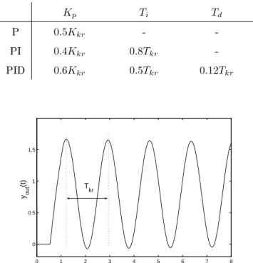
parameters are calculated using formulas in Table 1. Ultimate frequency method is based on determining the highest gainKkr that keeps the proportionally controlled closed-loop system stable. By determining

(7)

Tkr from the system output, as seen in Figure 3, we can calculate the PID controller parameters using formulas in Table 2. Both of these methods are designed using the quarter amplitude damping design criterion. [6]

Table 1: PID parameters according to the Ziegler Nichols step response method

Kp Ti Td P T KL1 - -PI _KL0.9T 1 3L1 -PID 1.2T KL1 2L1 0.5L1

Table 2: PID parameters according to the Ziegler Nichols ultimate frequency method

Kp Ti Td P 0.5Kkr - -PI 0.4Kkr 0.8Tkr -PID 0.6Kkr 0.5Tkr 0.12Tkr 0 1 2 3 4 5 6 7 8 0 0.5 1 1.5 time yout (t) T kr

Figure 3: Ziegler Nichols Ultimate Frequency Method parameters determination

3.2 Cohen and Coon Method

The Cohen and Coon tuning method is based on the same assumptions on the rst order system as the Ziegler Nichols method. Nevertheless, the tuning criteria and parameters are determined in a slightly

(8)

dierent way. The PID controller parameters are calculated using the gainK, the time constantT and the delayL1 of the rst order approximation of the process (2), but using the rules shown in Table 3.[4]

Table 3: PID controller parameters according to the Cohen and Coon method

Kp Ti Td P 1 K ¡T L1 + 0.33 ¢ - -PI 1 K ¡ 0.9T L1 + 0.083 ¢ L13.33 + 0.31(L1/T) 1 + 2.22(L1/T) -PID 1 K ¡ 1.35T L1 + 0.25¢ L12.5 + 0.46(L1/T) 1 + 0.61(L1/T) 0.37L1 1 + 0.19(L1/T)

3.3 AMIGO Method

AMIGO (Approximate M-constrained Integral Gain Optimization) tuning method uses a dierent PID control algorithm compared to the previous methods. Here ltering is applied on all terms, not only on the derivative part. The AMIGO controller is given as

u(t) =kp¡byr(t)−yf(t)¢+ki Z t 0 yr(α)−yf(α)dα+kd¡cdyr(t) dt − yf(t) dt ¢ , (5)

wherebandc are the set-point weights andyf is the ltered process output signal. yf is obtained from the process output signaly by ltering, i.e. Yf(s) =Gf(s)Y(s). The lter transfer function is

Gf(s) = 1

(1 +sTf)n, (6)

where Tf is the lter time constant and n= 1,2, .. is the lter of order. The AMIGO PID controller actually has six tunable parameterskp, ki, kd, Tf, bandc. The AMIGO tuning rules proposed by Åström and Hägglund in [8] are

Kp= 1 K ¡ 0.2 + 0.45T L1 ¢ Ti =L10.4L1+ 0.8T L1+ 0.1T Td= 0.5L1T 0.3L1+T (7)

where parameters K, T and L1 are determined by the rst order model in (2). Filter time constant is

set toTf ≈0.1L1 and the set point weights are set toc= 0 and

b=    0, if L1 T+L1 <0.5 1, if L1 T+L1 ≥0.5

Note thatkp=Kp,ki=Kp/Ti andkd=KpTd.

3.4 Lambda Tuning Method

Lambda tuning method is principally a pole placement method. The process model is assumed to be the rst order transfer function (2). The closed-loop transfer function of the process is desired to be of rst

(9)

Q(s)

G(s)

( )

G s

-+ + + + -y_r y d u y

Figure 4: Block diagram of IMC controller

order

Gcl(s) = K

1 +λse

−L1s (8)

whereλis the tuning parameter that determines the pole location. Smallerλvalues increase the controller performance but take it closer to the instability region. Now by using the rst order Taylor approximation on the delay and by settingTi=T we get the following PI controller tuning parameters (see Appendix A.2)

Kp= T

K(λ+L1), Ti=T. (9)

Similarly using Padé approximation of the delay we obtain tuning parameters for a PID controller as [2]

Kp= T+L1/2

K(λ+L1/2)

, Ti=T+L1/2, Td= T L1

L1+ 2T

. (10)

3.5 Internal Model Control Method

Internal Model Control (IMC) is a model based tuning method that utilizes a rst or higher order model of the process. It is the only model based tuning method we use that allows applying higher than rst order models. IMC controller consists of an estimator block G˜, a process G and the controller Q. A schematic block diagram of an IMC controller is illustrated in Figure 4. The system modelG˜ considered in this study was introduced in Section 2.1. The modelG˜(s)can be divided into two parts and written in form

˜

G(s) = ˜G+(s) ˜G−(s), (11)

where G˜+(s)is the non-invertible part of the transfer function and G˜−(s) is the invertible part. Thus,

all unstable zeros and delays of_G˜₍_s₎_{are included in}_G˜₊₍_s_{). Now the controller}_Q₍_s₎_{can be written in} form

Q(s) = ˜G−−1(s)f(s), (12)

wheref is a low-pass lter of desired ordern. Forf we can write

f(s) = 1

(1 +Tls)n, (13)

where Tl is the time constant of the lter andn is the lter order. The IMC control loop can also be represented in a classical control loop form with controllerC(s)as illustrated in Figure 5.

(10)

C(s)

G(s)

+

-y_r _u y

Figure 5: Block diagram of IMC controller Then, the controller transfer function becomes

C(s) = Q(s)

1−G˜(s)Q(s). (14)

Dividing the heated airow process model transfer function (1) into invertible and non-invertible parts yield to

˜

G+(s) =esL2, G˜−(s) = K

(Tas+ 1)(Tbs+ 1)

. (15)

Now, (12) can be written in the form

Q(s) = ˜G−−1(s)f(s) =

(Tas+ 1)(Tbs+ 1)

K(1 +Tls)n . (16)

Furthermore (14) can be written as

C(s) = 1

K

(Tas+ 1)(Tbs+ 1)

(1 +Tls)n₋_esL2 , (17)

where n should be selected such that the degree of denominator is greater or equal to the degree of numerator. So, herenshould be set ton≥2.

By approximating the delay with the Padé approximation

e−sL2 ₌1− 1 2L2s 1 + 1 2L2s (18) we can write (17) in form

C(s) = 1 K 1 2L2TaTbs3+ (TaTb+12L2(Ta+Tb))s2+ (Ta+Tb+12L2)s+ 1 1 2L2Tl2s3+ (Tl2+TlL2)s2+ (2Tl+L2)s . (19)

It should be noted at this point thatTl is the only tunable parameter in the controller. So the tuning of the controller reduces into nding the optimal value for parameterTl. The delaye−L2s could also be

approximated with a rst order Taylor polynomial which leads into Lambda PID controller introduced in previous Section. [3]

3.6 Practical PID Controller Design Aspects

When embedding the PID controller into a physical process such as our case process, the heated airow system, some design restrictions must be taken into consideration. We focus on three of those restrictions called integrator windup, measurement noise and nonlinearity.

(11)

Integrator windup occurs because the control signal is in practice bounded. In our process the heater control signal is bounded to the interval 0..10V. If the closed-loop process is controlled with a reference signal yr that exceeds the process maximum output ymax, a constant deviation remains in the error signal e(t). This causes the integral term, integrating the error signal to continuously increase, which directly causes the controller output signal to increase. While the actuator remains bounded, the integral term continues increasing and nally when the reference signalyr is set back to a feasible value it takes a relatively long time for the controller integral term to get back to normal value. Integrator windup can be prevented using integrator anti-windup, which measures the dierence between the PID controller output and the bounds of output if the signal is out of bounds. Upon actuator saturation the integral term is aected by the anti-windup mechanism to prevent the undesired behavior.

Measurement noise always occurs in physical measurements. The temperature measurement output signal of our process has substantially large noise. Measurement noise, especially noise with high fre-quency, inuences mostly on the PID controller derivative term, because it has an increasing frequency response. Hence, ltering needs to be applied at least on the controller derivative term as explained in Appendix A.1.

Nonlinearity in a system can be seen, for example, if the parameters of the process changes as a function of the operating point. In our process it can be seen that the static gain, for example, changes dramatically at high temperatures. Generally, the nonlinearities can be avoided by approximating the system to be linear at a small interval around certain operating point.

All computer-aided controllers are eventually discrete-time controllers. Discrete-time controllers are discrete approximations of the corresponding continuous-time controllers and thus contains always some error compared to the continuous time controllers. However, with modern microprocessors and measure-ment electronics the sampling interval can be so small that the error is very small. [6]

4 Tools for Analysis of Tuning Methods

The educational purpose of the PID control laboratory exercise is to give a clear and illustrative picture of the basic behavior and characteristics of PID controlled systems, to familiarize students with advantages and disadvantages of PID controllers and to introduce the tuning methods of PID controllers. To meet these requirements some comparison and analysis of the PID control methods needs to be performed. Our target is to choose a few of the methods introduced in Section 3 and use them rather than using all methods. It is also desired that the application area that is originally intended for each controller is illustrated. In order to be able to compare the methods, the performance criteria need to be set. In this work we focus on performance and robustness. This section briey reviews the chosen criteria.

(12)

4.1 Performance of Tuning Methods

There are several criteria that are used to measure controller performance. These methods more or less measure the total error between the system reference path and the real system path. The formulation of a performance measure can be represented in form

Ji(T) =

Z _T

0

h(e(t), u(t), t)dt, (20)

wheree(t)is the deviation from the path error,u(t)is the control signal andhis a weight function giving positive values. Dierent representations of performance measures are shown in Appendix B [1].

Another measure indicating system performance is the system settling time. Generally, settling time is determined as the time from which the error remains less than 2% of the reference value after the step change in reference. Nevertheless, sometimes it can be quite dicult to determine the settling time accu-rately. Especially, if the error signal oscillates or noise is present in the measurements, determining the instant when error is less than some xed value is very dicult and sensitive to variation of parameters. We measure the performance of each control method introduced in Section 3 and compare the methods using the performance measures presented here. It has to be noted that we compare only PI controllers with other PI controllers and PID controllers with other PID controllers. In general, it is reasonable to compare only controllers of same order. This is because theoretically controllers with higher order can be tuned to give at least as good results as controllers of lower order.

4.2 Sensitivity to Disturbances

The tuning methods might give good results in sense of the performance measures discussed in previous section, but no method is useful if the controlled system is sensitive to modeling errors, disturbances in control signal or measurement noise. System sensitivity analysis is another useful method to measure the quality and adequacy of the controllers. In this case we perform a sensitivity analysis based on the maximum sensitivity of the closed-loop system.

First we determine the sensitivity function and complementary sensitivity function for a closed-loop system. Let the controller transfer function beGc(s)and process transfer functionG(s). The sensitivity function of the system is then

S(s) = 1

1 +L(s), (21)

whereL(s) =Gc(s)G(s)is the transfer function of the open-loop system. The complementary sensitivity function can thus be formulated as

T(s) = L(s)

1 +L(s). (22)

It should be noted that by denitionT(s) +S(s) = 1.[1] The sensitivity function describes the system response sensitivity to reference signal changes, whereas the complementary sensitivity function describes the system sensitivity to measurement noise. Moreover, they describe the system sensitivity to modeling errors which is important to notice in this study.

(13)

It is shown in [7] and [8] that if the Nyquist Diagram of the open-loop systemL(s)and a circle with radius rR and center on negative real axis in cr do not intersect, the system sensitivity function S(s) and complementary sensitivity functionT(s)are less than or equal toM, where

rR= 2M−1 2M(M−1) (23) and cR=−2M 2₋₂_M _{+ 1} 2M(M −1) , (24)

where parameter M > 1. Thus, the parameter M can be interpreted as a parameter of sensitivity or equivalently robustness that expresses the maximum value of system sensitivity. Smaller values of M

make the circle radiusrRgreater, which takes the Nyquist curve further o from the critical point -1+i0

and makes the system more robust. On the contrary, greater values ofM decrease the radius rR and take the Nyquist curve closer to instability region. TypicallyM values of a robust system are at interval 1.2< M <2.0.[8]

5 Results

5.1 Process Model Parameter Estimation

The parameter estimation process of the system models described in Section 2.1 is performed with Matlab. Because of the nonlinearity of the real process and the inaccuracy of the utilized models it is desired that we choose a small bounded interval as operating interval as explained in Sections 2.1 and 4.2. We start the parameter estimation by determining the model parameters' P2 dependence on the

operation point. In the experiment setup we apply a step input of 1V into process and measure the response. This step response is determined at 10 points in the input range and the parametersP2 are

determined by solving (3). The results are shown in Figure 6. Parameter values seem to vary quite signicantly at both ends of the range. At 9V there was a lot of drifting in the measurement data which explains the deviation in the time parameter values. However, between input range 3-7V the parameter values seem to be quite stable and constant. So, it is reasonable to tune the controllers to operate at this interval. Thus, if we do not want time varying parameters or operation point dependent parameters, this is the best interval to perform controller tuning with methods that utilize the linear process model. The average values of process parameters at interval 3-7V are shown in Table 4. These values are used in the controller tuning that is discussed in the following section. The parameters P1 of the rst order model

(see (2) ) are estimated utilizing the second order model. Because the second order model approximates the process very well and the parameter valuesP2are quite stable at the chosen interval, it is reasonable

to assume that the rst order model also behaves in such manner. To perform the estimation process a suitable Matlab script was written. The script determines automatically the maximum of derivative function and calculates the parameters as described in Section 2.2. The values for parameters P1 are

(14)

Table 4: ParametersP2mean values and parameterP1values

P2 P1

parameter value parameter value

K 1.0888 K 1.0888

Ta 0.6004 T 0.6813

Tb 0.1276 L1 0.2287

L2 0.1617

5.2 Controller Parameters

Now, parameters for dierent controllers introduced in Section 3 can be calculated. This is performed with the rst and second order models of the process and the values of parametersP2andP1determined

in the previous section. For convenience, we divide the controller tuning methods into two categories. The rst category contains the tuning methods that have constant parameters and the second category contains the methods that have an adjustable tuning parameter. Thus, into the rst category we include Ziegler Nichols step response method and ultimate frequency method, Cohen and Coon method and AMIGO method. Into the second category we include the Lambda tuning method and the IMC tuning method. The controllers in the rst category are tuned rst. We concentrate on PI and PID controllers. The parameters for the controllers in the rst category are shown in Table 5. To illustrate the eciency of the tuning methods we performed simulations with the process model. This gives a rst hand information of the controller eects to the behavior of the actual process. We perform a more deeper comparison of the methods in the following section. We study the controller behavior in two

1 2 3 4 5 6 7 8 9 10 0 0.5 1 1.5 2 2.5 Parameter value

input operation point [V]

K T_a [s] T_b [s] L₂ [s]

(15)

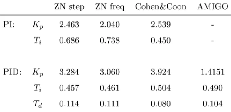
Table 5: Parameter values of category one controllers ZN step ZN freq Cohen&Coon AMIGO

PI: Kp 2.463 2.040 2.539

-Ti 0.686 0.738 0.450

-PID: Kp 3.284 3.060 3.924 1.4151

Ti 0.457 0.461 0.504 0.490

Td 0.114 0.111 0.080 0.104

cases; the load disturbance and reference signal tracking as mentioned in Section 3. Response of the closed-loop models to step change in reference signal are shown in Figure 7. Similarly, the closed-loop system responses to a load disturbance are shown in Figure 8.

In the second category, parameter values are determined only for Lambda controller. For IMC controller explicit parameter values cannot be determined, because the controller structure and parameter values depend signicantly on the process model structure. Parameter values for Lambda controller are determined such that we use four predetermined values forλ-parameter. These values have been selected with graphical inspection from system step response. The parameter values and correspondingλvalues can be seen in Table 6.

Table 6: Values of Lambda controller parameters Lambda λ= 0.1 λ= 0.2 λ= 0.3 λ= 0.6 PI: Kp 1.904 1.460 1.184 0.755 Ti 0.681 PID: Kp 3.401 2.325 1.764 1.023 Ti 0.796 Td 0.098

Determining the parameter values for IMC controller is more complicated. Even though the IMC controller reduces to PID controller when rst order process model is used, it is not practical to calculate the parameter values explicitly. The closed-loop response of the model when a step reference signal is applied with Lambda tuning and IMC controller is shown in Figures 9 and 11(a). Here we also use few predetermined values for parameterTl value, which can be seen in the gures. Similarly, the behavior of the system, when a load disturbance (1V step change in input signal) is applied is shown in Figures 10 and 11(b).

(16)

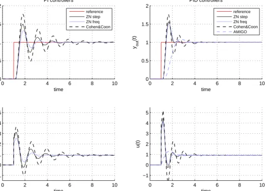
0 2 4 6 8 10 0 0.5 1 1.5 2 time yout (t) PI controllers reference ZN step ZN freq Cohen&Coon 0 2 4 6 8 10 −1 0 1 2 3 4 5 time u(t) 0 2 4 6 8 10 0 0.5 1 1.5 2 PID controllers time yout (t) reference ZN step ZN freq Cohen&Coon AMIGO 0 2 4 6 8 10 −1 0 1 2 3 4 5 time u(t)

Figure 7: Output and control signals of the closed-loop systems for dierent tuning methods when a step in reference signal is applied. Category one controllers.

0 2 4 6 8 10 −0.2 −0.1 0 0.1 0.2 0.3 0.4 0.5 time yout (t) PI controllers reference ZN step ZN freq Cohen&Coon 0 2 4 6 8 10 −1 −0.5 0 0.5 1 1.5 time u(t) 0 2 4 6 8 10 −0.2 −0.1 0 0.1 0.2 0.3 0.4 0.5 PID controllers time yout (t) reference ZN step ZN freq Cohen&Coon AMIGO 0 2 4 6 8 10 −1 −0.5 0 0.5 1 1.5 time u(t)

Figure 8: Output and control signals of the closed-loop systems for dierent tuning methods when a load disturbance is applied. Category one controllers.

(17)

0 1 2 3 4 5 6 7 8 9 10 0 0.5 1 1.5 o u tp u t y (t ) time O = 0.1 O = 0.2 O = 0.3 O = 0.6 y ref 0 1 2 3 4 5 6 7 8 9 10 -1 0 1 2 3 4 5 c o n tr o l u (t ) time 0 1 2 3 4 5 6 7 8 9 10 0 0.5 1 1.5 o u tp u t y (t ) time O = 0.1 O = 0.2 O = 0.3 O = 0.6 y ref 0 1 2 3 4 5 6 7 8 9 10 -1 0 1 2 3 4 5 c o n tr o l u (t ) time (a) (b)

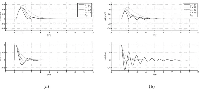
Figure 9: Closed-loop system output and control signals with Lambda tuned (a) PI (b) PID controller when a step of 1V is applied to reference att=1s.

0 1 2 3 4 5 6 7 8 9 10 -0.4 -0.2 0 0.2 0.4 0.6 o u tp u t y (t ) time O = 0.1 O = 0.2 O = 0.3 O = 0.6 y ref 0 1 2 3 4 5 6 7 8 9 10 -0.5 0 0.5 1 c o n tr o l u (t ) time 0 1 2 3 4 5 6 7 8 9 10 -0.4 -0.2 0 0.2 0.4 0.6 o u tp u t y (t ) time O = 0.1 O = 0.2 O = 0.3 O = 0.6 y ref 0 1 2 3 4 5 6 7 8 9 10 -0.5 0 0.5 1 c o n tr o l u (t ) time (a) (b)

Figure 10: Closed-loop system output and control signals with Lambda tuned (a) PI (b) PID controller when a load disturbance of 1V is applied att=1s.

(18)

0 2 4 6 8 10 0 0.2 0.4 0.6 0.8 1 output y(t) t T l: 0.1 T l: 0.2 T l: 0.3 T l: 0.6 y ref 0 2 4 6 8 10 0 2 4 6 8 control u(t) t 0 2 4 6 8 10 0 0.2 0.4 0.6 0.8 1 output y(t) t T l: 0.1 T l: 0.2 T l: 0.3 T l: 0.6 y ref 0 2 4 6 8 10 0 0.2 0.4 0.6 0.8 1 control u(t) t (a) (b)

Figure 11: Closed-loop output and control signals of the IMC controlled system in case of (a) reference tracking (step att=1s) (b) load disturbance rejection (step at t=1s)

5.3 Comparison of Controllers' Performance

We determine the controllers' performance with the methods introduced in Section 4.1 and Appendix B. As mentioned earlier, it is reasonable to compare only PI controllers with other PI controllers and PID controllers with other PID controllers. It is good to keep in mind that the performance measures determined here, loosely speaking, 'correlate' with the area between the reference signal and the output signal of the process seen in Figures 7 - 11. First we determine the performance measures for category one PI controllers in the case of reference signal tracking and load disturbance rejection. Results are shown in Figures 12 (a) and (b). The performance values are relative such that the best tuning method has value 1.00 and the other values are relative to this. Comparison of PI controllers in the case of reference signal tracking shows that Ziegler Nichols ultimate frequency method gives the best results in our performance tests. As seen in Figure 12 (a) Ziegler Nichols ultimate frequency method beats all other methods with all performance measures. In case of load disturbance the Ziegler Nichols step response method is the best in sense of all performance measures exceptJopt.

The performance measures for category one PID controllers in case of reference signal tracking and load disturbance rejection are shown in Figures 13 (a) and (b). The best PID controller tuning methods in case of reference signal tracking are Ziegler Nichols ultimate frequency method and step response method as shown in Figure 13 (a). They give almost equally good performance measures in case of all other performance measures except Jopt. The AMIGO PID controller is the best in case of the Jopt

performance measure.

In case of load disturbance rejection the situation is more complicated as seen in Figure 13(b). A clearly dominating controller in sense of all performance measures is dicult to determine among Ziegler Nichols and Cohen&Coon methods. Ziegler Nichols Step response method is best in case of absolute

(19)

1,12 1,00 1,00 1,00 1,00 1,84 1,62 1,26 1,79 1,00 5,54 2,22 1,78 3,81 6,27 0,00 1,00 2,00 3,00 4,00 5,00 6,00 7,00 J_itae: J_iae: J_ise: J_itse: J_opt:

ZN step ZN freq Cohen&Coon

1,00 1,00 1,00 1,00 1,02 1,00 1,28 1,24 1,11 1,03 1,60 1,52 1,15 1,32 2,62 0,00 0,50 1,00 1,50 2,00 2,50 3,00 J_itae: J_iae: J_ise: J_itse: J_opt:

ZN step ZN freq Cohen&Coon

(a) (b)

Figure 12: Relative performance values for category one PI controllers in case of (a) reference signal tracking (b) load disturbance rejection

4,57 1,00 1,00 1,02 1,00 1,00 1,00 1,00 1,00 3,90 2,61 1,77 1,41 1,22 8,68 2,26 1,76 1,60 2,42 1,00 0,00 1,00 2,00 3,00 4,00 5,00 6,00 7,00 8,00 9,00 J_itae: J_iae: J_ise: J_itse: J_opt:

ZN step ZN freq Cohen&Coon AMIGO

1,00 1,10 1,13 1,02 1,00 1,04 5,68 1,00 1,02 1,00 1,00 1,01 1,08 1,15 1,82 1,06 1,25 4,41 3,99 2,79 0,00 1,00 2,00 3,00 4,00 5,00 6,00 J_itae: J_iae: J_ise: J_itse: J_opt:

ZN step ZN freq Cohen&Coon AMIGO

(a) (b)

Figure 13: Relative performance values for category one PID controllers in case of (a) reference signal tracking (b) load disturbance rejection

(20)

error performance measures, but Cohen&Coon seems to be the best in case of squared error performance measures, although, the dierences are small. AMIGO PID controller is not very good in sense of performance measures based on absolute and squared error, but it is dominating in case of the Jopt

performance measure.

Settling times ts of the category one controllers are listed in Appendix C.1. The shortest settling times seem to be achieved with Ziegler Nichols methods. In the worst case, the Cohen & Coon method seems to have twice as long settling times as Ziegler Nichols methods.

For category two controllers we determined the performance measure values using dierent values for the tunable parameter. Thus, the performance measures were determined with small separation of tunable parameter and then plotted as function of the parameter to illustrate the performance behavior. Performance values for Lambda PI controller in case of reference signal tracking are shown in Figure 14 (a) and the corresponding Lambda PID controller performance values are seen in Figure 14 (b). Performance of the PID controllers seems to be slightly better at all values ofλin sense of all performance measures. Performance values for Lambda PI controller in case of load disturbance are shown in Figure 15 (a) and the corresponding Lambda PID controller performance values are seen in Figure 15 (b). Similarly Lambda PID controller performance values are slightly better for all values ofλ.

Performance values of the IMC controller are shown in Figures 16 (a) and (b). Compared to the Lambda controllers the performance values seem to increase very rapidly when parameterTl increases but at the same time the decrease in theM-value is very gradual. This indicates that the IMC controller is more sensitive to variations of the tunable parameterTl. There also seem not be a similar minimum values for performance measures as the Lambda controllers have in case of reference signal tracking.

A summary of performance numbers and settling times is shown in Appendix C.1.

0 0.2 0.4 0.6 0.8 1 0 0.5 1 1.5 2 2.5 3 3.5 4 λ M / J J_itae J_iae J_ise J_itse J_opt M−value 0.1 0.2 0.3 0.4 0.5 0.6 0.7 0.8 0.9 0 0.5 1 1.5 2 2.5 3 3.5 λ M / J J_itae J_iae J_ise J_itse J_opt M−value (a) (b)

Figure 14: M values and cost function values (in case of reference signal tracking) as functions ofλfor (a) PI controller (b) PID controller

(21)

0 0.2 0.4 0.6 0.8 1 0 1 2 3 4 5 6 lambda M / J cost J_itae J_iae J_ise J_itse J_opt M−value 0.1 0.2 0.3 0.4 0.5 0.6 0.7 0.8 0.9 0 1 2 3 4 5 6 lambda M / J cost J_itae J_iae J_ise J_itse J_opt M−value (a) (b)

Figure 15: M values and cost function values (in case of load disturbance rejection) as functions ofλfor (a) PI controller (b) PID controller

0 0.2 0.4 0.6 0.8 1 0 0.5 1 1.5 2 2.5 3 3.5 T_f M / J cost J_itae J_iae J_ise J itse J opt M−value 0 0.2 0.4 0.6 0.8 1 0 1 2 3 4 5 6 T f M / J cost J itae J iae J_ise J_itse J opt M−value (a) (b)

Figure 16: M-values and cost function values of IMC controller as functions of parameterTl in case of (a) reference signal tracking and (b) load disturbance rejection

(22)

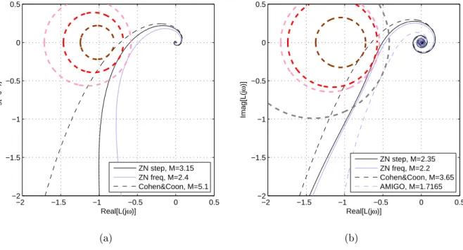
−2 −1.5 −1 −0.5 0 0.5 −2 −1.5 −1 −0.5 0 0.5 Real[L(jω)] Imag[L(j ω )] PI controllers ZN step, M=3.15 ZN freq, M=2.4 Cohen&Coon, M=5.1 −2 −1.5 −1 −0.5 0 0.5 −2 −1.5 −1 −0.5 0 0.5 Real[L(jω)] Imag[L(j ω )] PID controllers ZN step, M=2.35 ZN freq, M=2.2 Cohen&Coon, M=3.65 AMIGO, M=1.7165 (a) (b)

Figure 17: Nyquist diagrams andM-circles for (a) PI and (b) PID controllers

5.4 Comparison of Controllers' Sensitivity

Sensitivity of controllers is also analyzed separately for category one and category two controllers. For category one controllers the Nyquist diagrams and the M-circles are plotted in Figure 17. Controllers with greaterM values (smaller circles) are more sensitive to disturbances and measurement noise than ones with smallerM values (larger circles).

For category two controllers the M-values were also determined as a function of tunable parameter. In Figures 14 - 15 theM-value is plotted as a function ofλin the same gure with controller performance function values that were determined in last section. M-values are naturally equal for PI controllers in both cases, the reference signal tracking and the load disturbance rejection. SimilarlyM-values are equal for PID controllers in both cases as the controllers and the plant are the same.

M-values of the IMC controller are plotted together with the controller performance costs as a function of the parameterTf in Figure 16 (a)-(b). TheM-curve is same in both gures (a) and (b) but the costs are dierent in the two cases.

By plotting the controllers M-values and settling times into same gure gives good picture of the trade-o between robustness and performance. All controllers plotted inM-tsplane are shown in Figure 18. In case of tunable parameter controllers we have chosen the ones with best values by weighting

M-value and settling time with equal weights. It should be noted that only tuning methods that reach the area of good robustness (1 < M ≤2) are the AMIGO method and tunable parameter controllers. However, as mentioned earlier the settling time can be considered only as an approximative performance indicator. Furthermore, to compare the theoretical goodness of tuning methods we have plotted theJiae

(23)

ZN step PI

ZN step PID ZN freq PI

ZN freq PID Cohen&Coon PI Cohen&Coon PID AMIGO Lambda PI Lambda PID IMC 0 1 2 3 4 5 6 0 1 2 3 4 5 6 7 8 9 Settling time [s] M -v a lu e

Figure 18: Controllers'M-value versus settling time. Better controllers are near origo

measure in load disturbance rejection case versus the Jise in reference tracking case in Figure C.13 in Appendix. Jiae andJiseare typically used to measure the performance in the case of load disturbance rejection and reference tracking, respectively. Thus, Figure C.13 illustrates if the controller is more suitable to reference tracking or load dsturbance rejection. The performance measures Jiae, Jise and

Jopt are also plotted versus theM value in Figures C.14 - C.16 in Appendix. These gures show that in this case the Ziegler Nichols methods seems to be very good in both PI and PID controllers. On the contrary, the Cohen and Coon methods seem to be quite poor in all cases. The tunable methods seems to be better than other methods in case of reference tracking, but in load disturbance rejection they can only reach the performance of the Ziegler Nichols methods. The ranking of AMIGO method is quite tricky. In case of Jopt performance measure it is superior and in load disturbance rejection it reaches quite good results, but in reference signal tracking it is very poor. A summary of theM-values of the category one controllers is shown also in Appendix C.1.

5.5 Applying Methods to the Heated Airow Process

After a thorough study of tuning methods and their applicability to the process model we lack only the knowledge of how the actual process can be controlled with the methods. Next, we perform tests with the process that are based on the results we have found with the process modeling. Implementing rst the controller algorithms into Matlab using xPC Target toolbox, a real-time process control and measurement system, we can test the behavior of the controlled process. The response given by the simulation of the second order model and the actual process are plotted in same gure in Appendix

(24)

C.2 for all controllers. For tunable parameter controllers we have chosen controllers that are good representatives or compromises of controllers with good performance and robustness. The actual process and simulation results seem to meet each other relatively well, especially in the case of load disturbance rejection. The gures show that the static gain of the system and the output delay were estimated very well. However, in case of reference signal tracking the actual process seems to settle to steady state value faster than the estimated model predicts. It is also noticed that in the case of PID controllers the measurement noise is not ltered very well in the feedback loop and hence the noise in the control signal

u(t)is signicantly large. The noise could be reduced with increasing the measurement signal ltering but this would decrease the controller performance.

6 Educational Discussion

In this section we discuss the essential guidelines and practical results we have found to be important in developing a laboratory course exercise on PID control for undergraduate students.

From the laboratory exercise point of view it is important to give students knowledge about the basic behavior of the closed-loop system dynamics and PID controllers and to give illustrative examples of their behavior. Furthermore, explaining the background and preconditions for usage of tuning methods as well as giving reasons for their usage is necessary to make students understand the conditions in which the usage of PID controllers is useful. The aim is to advise students to use the methods properly and to learn the advantages and drawbacks of the PID controllers. However, it should be kept in mind that introducing too many methods and controllers might be confusing and make it dicult to distinguish relevant issues from rather irrelevant issues.

Students are expected to know the basics of the process dynamics and they most probably also know something about the PID controllers. For example the eects of measurement delay, especially in a closed-loop process and the shortcoming of a simple P controller which leaves a constant error between process output and reference signal. Some student might also be familiar with the eects that appear in the closed-loop system output when the controller parameters are varied. Particularly, greater P-term makes the closed-loop system more rapid, the I-term can be used to overcome the problems related to simple P controller, but it increases the oscillation of the output signal and the oscillations (caused by I-term and measurement delay) can be reduced with the D-term. It is important to distinguish the variation of parametersKp, Ti, Td and N and terms (P, I and D) because varying Kp aects all terms

as explained in Section 3. However, these eects can be demonstrated with the computer controlled process very easily and the eects of changing each parameter separately can be powerfully visualized. Also the possibility to vary certain process parameters, measurement delay and airow speed, makes the demonstration of process dynamics more versatile.

The process identication is the rst part of the tuning methods' application. In this work we have studied rst and second order models. These models explain the process behavior suciently for

(25)

controller tuning purposes. But, it should be noted that these models are quite simple and do not take into account for instance process parameter variation. This means that the process model must be re-estimated in case some of the process parameters change.

The parameter tuning of a basic PID controller can be performed with the methods introduced in this work. These tuning methods provide a good starting point for students to learn the PID controller. However, it should be noticed that the PID tuning methods give only a good approximative values for controller parameters. These values should be used mainly as a good initial estimate for parameters rather than optimal or nal values. Hence the manual adjustment of parameters is at least as important part of the controller tuning as the application of the tuning methods. Actually the manual adjustment could be considered as the eventual ne tuning method that can be used to set the controller to behave as desired. Nevertheless, incorporating the robustness measures into the analysis in the simulation phase, as was done in this study, provides deeper understanding of dierent methods and may even decrease the need for manual ne tuning when implementing the controllers.

As we found out in this project work, none of the basic tuning methods is superior to others in sense of both robustness and performance. Thus the relation between these properties requires clarication and students should understand the trade-o between the robustness and performance. In other words, it has to be emphasized that increasing the performance of a controller always makes the system more sensitive. This is because the performance is achieved by strengthening the feedback which makes the system behavior more rapid. With tunable parameter controllers it is easy to demonstrate the change in controller behavior, because the tuning can be reduced into changing one parameter.

One of the most noticeable characteristics of the case process is the noise in temperature measurement. This is mainly caused by the turbulence in the owing air which is not included into the system model as mentioned in Section 2.1. Noise is of course an undesired property in any part of a process, because it decreases the measurement accuracy and it has a destabilizing eect especially if the process includes feedbacks. Thus, dierent noise ltering methods can be used in the case process and the eects are very observable because the measurement noise of the case process is substantially large. The students are expected to have some knowledge of the concept of noise and probably the means to reduce it. At least they should know that noise is a high frequency variation in the measurement signal and they should be able to distinguish noisy measurement signal from a less noisy measurement.

In the case of a simple PID controller (4) the noise aects the D-term signicantly. It is easy to visualize that high frequency in signal means also high frequency in the derivative signal. So, including the D-term into a well functional PI controller can cause a large noise in the controller output signalu(t) and can lead even to instability of the process. Low-pass ltering of the measurement signal provides a solution to this problem. The controllers introduced in this work contain the low-pass lter. However, the tuning methods do not determine any values to lter parameters except the AMIGO method that determines an approximative value for Tf. This is because the strength of ltering depends on the existing noise and should be determined in all situations according to the characteristic process noise.

(26)

In tunable parameter controllers the ltering is included into controller and changes when adjusting the tunable parameter. So, including a proper lter increases the controller robustness but at the same time it makes the system response slower.

In Section 5.2 we already divided the studied controllers into two categories. This division is very good starting point in teaching the methods, although it is not yet necessary to decide the methods that should be nally used in the laboratory exercise. Category one tuning methods are very good to illustrate the behavior and dierences between the tuning methods. By illustrating both of the cases, the reference signal tracking and load disturbance rejection, it is evident for students that none of the methods is superior to others in sense of both performance and robustness. This could also be demonstrated with the robustness-performance maps shown in Appendix C.3. Category two controllers have a little more complex structure, but they are very useful in demonstrating the eects of controller tuning on the robustness and performance. This is because the controller tuning nally reduces to varying one parameter which determines the controller position in robustness-performance map.

7 Summary and Conclusions

In this research project we have performed a comprehensive study over the PID controller tuning on a heated airow process. Motivation for the study was the demand to develop a laboratory course exercise for undergraduate students. Several controllers and controller tuning methods described in this work were found out to be suitable for controlling the case process. Comparison of controllers performance and robustness proved that none of the controllers were superior to others. Thus, dierent controllers and tuning methods should be used in dierent situations. Measurement noise and process parameters variation also aect the controller performance and robustness. Controllers with high performance are usually sensitive to noise. Trade-o between robustness and performance makes the decision making among controllers more dicult.

The prospective development of the laboratory exercise will concentrate on writing the exercise in-structions and implementing the measurement software. Results of this work will be used to guide the determination of the exercise instructions. Especially this study gives basis for examination of the controllers robustness and performance. During the study of the tuning methods and process model estimation we have also implemented several Matlab scripts and Simulink models to perform the model parameter estimation automatically. These will be utilized in the measurement software development.

(27)

References

[1] Dorf R. C. and Bishop R. H., Modern Control Systems, Ninth Edition, Prentice Hall, 2001 [2] Eriksson L., Control Design and Implementation of Networked Control Systems, Licentiate thesis,

Department of Automation and Systems Technology, Helsinki University of Technology, May 2007. [3] Garcia C. E. and Morari M., Internal Model Control. 1. A Unifying Review and Some New Results, Industrial & Engineering Chemistry Process Design and Development, vol. 21, pp. 308-323, 1982 [4] O'Dwyer, A., Handbook of PI and PID Controller Tuning Rules, Imperial College Press, 2003 [5] Visioli A., Practical PID Control, Springer, 2006

[6] Åström K.J. and Hägglund T., Automatic Tuning of PID Controllers, Instrument Society of Amer-ica, 1988

[7] Åström K.J., Panagopoulos H. and Hägglund T., Design of PI Controllers based on Non-Convex Optimization, Automatica, Vol. 34, No. 5, pp. 585-601, 1998

[8] Åström K.J. and Hägglund T., Revisiting the Ziegler-Nichols step response method for PID control, Journal of Process Control 14 (2004) 635-650, Elsevier, 2004

(28)

Appendix

A PID Controllers

A.1 Formulations of Controllers

Equation (4) is sometimes also presented in the form

u(t) =kpe(t) +ki

Z _T

0

e(t)dt+kd d

dte(t), (A.1)

wherekp, kiandkdare the proportional, integral and derivative gains, respectively. The transfer function representation of a basic PID controller is

Gpid(s) =u(s) e(s) =Kp £ 1 + 1 Tis+Tds ¤ . (A.2)

The general sum representation of a PID controller is

u(s) =£up(s) +ui(s) +ud(s)¤e(s), (A.3) whereup(s)is the proportional term,ui(s)is the integral term andud(s)is the derivative term. These terms can be written in the form

up(s) =Kp, ui(s) =

Kp

Tis and ud(s) =KpTds.

The derivative term ud(s) can be modied such that it contains a low pass lter. This increases the robustness of the controller when the measured signal contains comparatively high frequency noise. The modied derivative term is

ud(s) = KpTds

1 +sTd/N,

whereN is the lter time constant, typically chosen in rangeN∈[3,20].

A.2 Lambda Tuning Method Parameters

Using the rst order approximation of the process

G(s) = K T s+ 1e −sL1_, (A.4) and PI controller GP I(s) =Kp 1 +Tis Tis , (A.5)

we obtain the closed-loop transfer function

Gc(s) = GP I(s)G(s)

1 +GP I(s)G(s). (A.6)

Now by setting the integrator time constantTiequal to the process time constantT and using rst order

Taylor approximatione−sL1= 1−sL₁ the closed-loop transfer function can be written in form

Gc(s) = KpK(1−sL1)

(29)

Thus the characteristic equation of the closed-loop system is

s(T−KpKL1) +KpK= 0, (A.8)

which gives a pole

s=− KpK

T−KpKL1. (A.9)

The pole of the closed-loop system is now set to the pole of the desired closed-loop system (s=−1/λ) and we get

1

λ=

KpK

T−KpKL1. (A.10)

Now writing this as function ofKp we get

Kp=

T

K(λ+L1)

. (A.11)

B Performance Measure Formulations

Performance measure based on error term absolute value

Jiae(T) =

Z T

0

|e(t)|dt (B.1)

Performance measure based on error square value

Jise(T) =

Z _T

0

(e(t))2dt (B.2)

Performance measure based on error absolute value weighted with time

Jitae(T) =

Z T

0

t|e(t)|dt (B.3)

Performance measure based on error square value weighted with time

Jitse(T) =

Z T

0

t(e(t))2_dt _(B.4)

Performance measure based on weighted sum of error square value and square of control signal deviation

Jopt(T) =

Z _T

0

w1e(t)2+w2[yr(t)−Ku(t)]2dt, (B.5)

(30)

C Additional Tables and Figures

C.1 Controller M-values and Performances

ZN step ZN step ZN freq ZN freq Cohen&Coon Cohen&Coon AMIGO

PI PID PI PID PI PID PID

Settling time [s] 4.65 2.63 4.03 2.16 8.07 4.12 3.44

M-value 3.15 2.35 2.40 2.20 5.10 3.65 1.72

Reference tracking performance (relative)

Jitae 1.84 1.02 1.00 1.00 6.27 2.61 2.26

Jiae 1.26 1.00 1.00 1.00 2.22 1.41 1.60

Jise 1.12 1.00 1.00 1.00 1.78 1.22 1.76

Jitse 1.62 1.00 1.00 1.00 5.54 1.77 2.42

Jopt 1.79 4.57 1.00 3.90 3.81 8.68 1.00

Load disturbance performance (relative)

Jiae 1.00 1.00 1.03 1.10 2.62 1.82 4.41

Jiae 1.00 1.00 1.11 1.08 1.52 1.25 2.79

Jise 1.00 1.01 1.24 1.13 1.15 1.06 5.68

(31)

C.2 Closed-loop System Output and Control Signals for Category One

Con-trollers

0 2 4 6 8 10 0 0.5 1 1.5 output y(t) time y out PI 0 2 4 6 8 10 −1 0 1 2 3 4 5 control u(t) time 0 2 4 6 8 10 0 0.5 1 1.5 output y(t) time y out PID 0 2 4 6 8 10 −1 0 1 2 3 4 5 control u(t) time (a) (b)

Figure C.1: Model simulation output and process output of the closed-loop system when the (a) PI and (b) PID controllers are tuned with Ziegler Nichols step response method. The noisy signal is the process output signal and the smooth signal is the model simulation output signal.

Figure C.2: Model simulation output and process output of the closed-loop system when the (a) PI and (b) PID controllers are tuned with Ziegler Nichols ultimate frequency method

(32)

Figure C.3: Model simulation output and process output of the closed-loop system when the (a) PI and (b) PID controllers are tuned with Cohen & Coon method

0 2 4 6 8 10 0 0.5 1 1.5 output y(t) time 0 2 4 6 8 10 −1 0 1 2 3 4 5 control u(t) time

Figure C.4: Model simulation output and process output of the closed-loop system with AMIGO PID controller

(33)

0 2 4 6 8 10 −0.4 −0.2 0 0.2 0.4 0.6 output y(t) time y out PI 0 2 4 6 8 10 −0.5 0 0.5 1 control u(t) time 0 2 4 6 8 10 −0.4 −0.2 0 0.2 0.4 0.6 output y(t) time y out PID 0 2 4 6 8 10 −0.5 0 0.5 1 control u(t) time (a) (b)

Figure C.5: Model simulation output and process output of closed-loop system with (a) PI (b) PID controller tuned with Ziegler Nichols step response method when a load disturbance of 1V at t=1s is applied 0 2 4 6 8 10 −0.4 −0.2 0 0.2 0.4 0.6 output y(t) time y out PI 0 2 4 6 8 10 −0.5 0 0.5 1 control u(t) time 0 2 4 6 8 10 −0.4 −0.2 0 0.2 0.4 0.6 output y(t) time y out PID 0 2 4 6 8 10 −0.5 0 0.5 1 control u(t) time (a) (b)

Figure C.6: Model simulation output and process output of closed-loop system with (a) PI (b) PID controller tuned Ziegler Nichols ultimate frequency method when a load disturbance of 1V at t=1s is applied

(34)

0 2 4 6 8 10 −0.4 −0.2 0 0.2 0.4 0.6 output y(t) time y out PI 0 2 4 6 8 10 −0.5 0 0.5 1 control u(t) time 0 2 4 6 8 10 −0.4 −0.2 0 0.2 0.4 0.6 output y(t) time y out PID 0 2 4 6 8 10 −0.5 0 0.5 1 control u(t) time (a) (b)

Figure C.7: Model simulation output and process output of closed-loop system with (a) PI (b) PID controller tuned with Cohen & Coon method when a load disturbance of 1V att=1s is applied

0 2 4 6 8 10 −0.4 −0.2 0 0.2 0.4 0.6 output y(t) time 0 2 4 6 8 10 −0.5 0 0.5 1 control u(t) time

Figure C.8: Model simulation output and process output of closed-loop system with AMIGO PID con-troller when a load disturbance of 1V is applied att=1s.

(35)

0 2 4 6 8 10 0 0.5 1 1.5 output y(t) time y out PI λ=0.3 0 2 4 6 8 10 −1 0 1 2 3 4 5 control u(t) time 0 2 4 6 8 10 0 0.5 1 1.5 output y(t) time y out PID λ=0.3 0 2 4 6 8 10 −1 0 1 2 3 4 5 control u(t) time (a) (b)

Figure C.9: Model simulation output and process output of a closed-loop system with (a) PI and (b) PID controller tuned with Lambda method (λ= 0.3) in case of reference signal tracking

0 2 4 6 8 10 0 0.5 1 1.5 output y(t) time y out PI λ=0.3 0 2 4 6 8 10 −1 0 1 2 3 4 5 control u(t) time 0 2 4 6 8 10 0 0.5 1 1.5 output y(t) time y out PID λ=0.3 0 2 4 6 8 10 −1 0 1 2 3 4 5 control u(t) time (a) (b)

Figure C.10: Model simulation output and process output of a closed-loop system with (a) PI and (b) PID controller tuned with Lambda method (λ= 0.3) when a load disturbance is applied

(36)

0 2 4 6 8 10 0 0.5 1 1.5 output y(t) time y out Tl=0.2 0 2 4 6 8 10 −1 0 1 2 3 4 5 control u(t) time 0 2 4 6 8 10 −0.4 −0.2 0 0.2 0.4 0.6 output y(t) time y out Tl=0.2 0 2 4 6 8 10 −0.5 0 0.5 1 control u(t) time (a) (b)

Figure C.11: Model simulation output and process output of a closed-loop system with IMC controller (Tl= 0.2) in the case of (a) reference signal tracking and (b) load disturbance rejection

0 2 4 6 8 10 0 0.5 1 1.5 output y(t) time y out Tl=0.3 0 2 4 6 8 10 −1 0 1 2 3 4 5 control u(t) time 0 2 4 6 8 10 −0.4 −0.2 0 0.2 0.4 0.6 output y(t) time y out Tl=0.3 0 2 4 6 8 10 −0.5 0 0.5 1 control u(t) time (a) (b)

Figure C.12: Model simulation output and process output of a closed-loop system with IMC controller (Tl= 0.3) in the case of (a) reference signal tracking and (b) load disturbance rejection

(37)

C.3 Performance and Robustness Comparison

ZN step PI ZN step PID ZN freq PI ZN freq PID Cohen&Coon PI Cohen&Coon PID AMIGO 0,0 0,2 0,4 0,6 0,8 1,0 0,0 0,2 0,4 0,6 0,8 1,0 J_iae load J _ is e r e f

Lambda PI Lambda PID IMC

Figure C.13: Controller performanceJisein reference tracking versusJiae in load disturbance rejection.

ZN step PI ZN step PID ZN freq PI ZN freq PID Cohen&Coon PI Cohen&Coon PID AMIGO 0 1 2 3 4 5 6 0 1 2 3 4 J_opt [s] M -v a lu e

LAMBDA LAMBDA IMC

(38)

ZN step PI ZN step PID ZN freq PI ZN freq PID Cohen&Coon PI Cohen&Coon PID AMIGO 0 1 2 3 4 5 6 0,0 0,2 0,4 0,6 0,8 J_ise [s] M -v a lu e

LAMBDA LAMBDA IMC

Figure C.15: M-values versus controller performanceJise in case of reference tracking.

ZN step PI ZN step PID ZN freq PI ZN freq PID Cohen&Coon PI Cohen&Coon PID AMIGO 0 1 2 3 4 5 6 0,0 0,2 0,4 0,6 0,8 1,0 1,2 1,4 Jiae [s] M -v a lu e

LAMBDA LAMBDA IMC load