The Rolling Tide Evolutionary Algorithm:
A Multi-Objective Optimiser
for Noisy Optimisation Problems
Jonathan E. Fieldsend
Member, IEEE
and Richard M. Everson
Abstract—As methods for evolutionary multi-objective optimi-sation (EMO) mature and are applied to a greater number of real world problems, there has been gathering interest in the effect of uncertainty and noise on multi-objective optimisation. Specifically, how algorithms are affected by it, how to mitigate its effects, and whether some optimisers are better suited to dealing with it than others. Here we address the problem of uncertain evaluation, where the uncertainty can be modelled as additive noise in objective space. We develop a novel algo-rithm, the rolling tide evolutionary algorithm (RTEA), which progressively improves the accuracy of its estimated Pareto set, whilst simultaneously driving the front towards the true Pareto front. It can cope with noise whose characteristics change as a function of location (both design and objective), or which alter during the course of an optimisation. Four state-of-the-art noise-tolerant EMO algorithms, as well as four widely used standard EMO algorithms, are compared to RTEA on 70 instances of ten continuous space test problems from the CEC’09 multi-objective optimisation test suite. Different instances of these problems are generated by modifying them to exhibit different types and intensities of noise. RTEA is seen to provide competitive performance across both the range of test problems used, and noise types.
I. INTRODUCTION
Evolutionary computation (EC) techniques are now exten-sively used when attempting to discover the optimal or near-optimal parametrisation for problems with complex function transformation from parameters (design variables) to objec-tive(s). Almost all optimisation procedures search the parame-ter space by evaluating the objectives for a given parametrisa-tion before proposing a new, hopefully better, parametrisaparametrisa-tion. It is generally assumed that repeated evaluation of the objec-tives for a single parametrisation yields the same objective val-ues. However, in many problems there is additional uncertainty in the veracity of the results obtained from the system model. Clear examples arise in “embodied” optimisation [1], [2], [3], where measurement error or stochastic elements in a physical system leads to different results for repeated evaluations at the same parameter values [4], [5] or when the objectives are derived from Monte Carlo simulations or data-driven systems [6], [7].
The authors are with the College of Engineering, Mathematics and Physical Sciences, University of Exeter, Exeter, EX4 4QF, UK (e-mail:
{J.E.Fieldsend,R.M.Everson}@exeter.ac.uk). Copyright (c) 2014 IEEE. Per-sonal use of this material is permitted. However, permission to use this material for any other purposes must be obtained from the IEEE by sending a request to [email protected].
Work in the scalar optimisation EC community to tackle these types of problem has indicated that elitist techniques often prove fragile [8], [9], [10], as there is no longer the guarantee that fitness of the elite solution improves as an optimiser progresses. As most modern multi-objective evolutionary al-gorithms (MOEAs) rely heavily on elitism, this should be of concern when optimising uncertain multi-objective problems. As early as 1993, the effect of noise on multi-objective optimisation was being considered, with Horn & Nafpliotis (at the end of [11]), discussing the ways in which uncertainty in an evaluation might be tackled. However, it was not until the early 2000s that a significant number of multi-objective opti-misers began to be developed specifically to tackle uncertain optimisation [12], [13], [14], [5], [6], [15], [7], [16], [17], [18], [19], [20], [21], [22], [23]. Typically uncertainty is modelled as noise added to the function evaluations, although recent work has begun looking at the situation where the objective functions themselves are uncertain [24].
In this paper we model the uncertainty in the objectives as observational noise. For the reader interested in the effect and mitigation of parametrisation uncertainty (often referred to as robust optimisation, or reliablity-based optimisation [25]), we recommend the work of Deb & Gupta [26]. This is also distinct from dynamic optimisation [27], in which the objectives change with time, but there is no uncertainty about each objective evaluation. The algorithm we examine here does, however, allow for dynamic noise characteristics; see also [6]. From here on we will use the term ‘optimisation with uncertainty’ as shorthand for objective uncertainty, which is the focus of this work.
We describe the multi-objective optimisation problem and some different types of observational noise which may be experienced in Section II, and in Section III we examine the effect of noise on a number of popular multi-objective evolu-tionary algorithms (MOEAs) – namely the Non-Dominated Sorting Genetic Algorithm II (NSGA-II) [28], the Pareto Archived Evolution Strategy (PAES) [29], the Strength Pareto Evolutionary Algorithm 2 (SPEA2) [30] and the Indicator-Based Evolutionary Algorithm (IBEA+) [31]. In Section IV we briefly describe some MOEAs that have been developed to cope with different types of observational noise prior to introducing our new algorithm, the rolling tide evolutionary algorithm (RTEA) in Section V.
other recent noise-tolerant MOEAs [6], [16], [21], [22], on standard test problems modified by the addition of noise. In particular we show that our proposed optimiser performs well in the presence of noise with a wide range of characteristics, including when the noise varies spatially and temporally during the course of the optimisation. We conclude with a discussion in Section VII.
II. MULTI-OBJECTIVE OPTIMISATION AND NOISE
Before discussing the effect of uncertainty in the evaluation of objectives, we briefly review the ideas of dominance and Pareto optimality which are central to multi-objective optimi-sation.
A general multi-objective optimisation problem seeks to si-multaneously extremise D objectives: fd(x), d = 1, . . . , D
where each objective depends upon a vector x = (x1, . . . , xk, . . . , xK)of K parameters or design variables.
The parameters may also be subject to equality and inequality constraints which, for simplicity, we assume can be evaluated precisely. When the objectives are to be minimised, the multi-objective optimisation problem may thus be expressed as:
minimise f(x) = (f1(x), . . . , fD(x)) (1)
with x ∈ X ⊆ RK, the feasible domain as defined by the constraints. When faced with only a single objective an optimal solution is one which minimises the objective given the model constraints. However, when there is more than one objective to be minimised, solutions may exist for which performance on one objective cannot be improved without reducing performance on at least one other. Such solutions are said to bePareto optimal.
The notion of dominance may be used to make Pareto opti-mality clearer. Assuming, without loss of generality, that the goal is to minimise the objectives and there is no noise, a design vector xis said to strictly dominateanotherx0 iff
fd(x)≤fd(x0) ∀d= 1, . . . , D and f(x)6=f(x0). (2)
This is often denoted asx≺x0 (as opposed tof(x)≺f(x0)). A set of design vectors A is said to be a mutually
non-dominating set if no member of the set is dominated by any
other member. A solution to the minimisation problem (1) is thus Pareto optimal if it is not dominated by any other feasible solution, and the non-dominated set of all Pareto optimal solutions is the Pareto setP.
The Pareto dominance notation can also be extended to sets (see e.g. [32]). This leads to a larger number of distinctions; however the set comparison we need here is: A≺B, which signifies that everyx∈Bis dominated by at least one member of A.
In this paper we are concerned with problems in which the objectives themselves are unobservable, but instead we have access to yd the objectives contaminated by observational
noise:
yd=fd(x) +d. (3)
We assume throughout that the observational noise encoun-tered at each evaluation is independent of other evaluations. The imposition of noise in an optimisation environment means that the dominance relationship calculated between solutions may be incorrect. Prior to discussing its effects it is useful to consider the different typesof observational noise that might be experienced in a particular industrial problem.
A. Unknown noise
The most severe case is when the noise characteristics are completely unknown. It may be asymmetric, it may be multi-modal, and there may be dependencies between noise in different objectives. Therefore, it could well be the case that the mean of a number of re-evaluations of y is a very poor approximation to f(x). In this case the degree of dominance between two solutions can only reasonably be estimated by repeated evaluation at the fixed parameter values x and x0.
Suppose thatY(x) ={yi}ni=1,are the noisy objectives eval-uated n times atx, and Y(x0) = {y0i}n0
i=1 are n0 evaluations atx0, then the probability thatxdominatesx0 is estimated by the fraction of times thatyi dominates y0j:
p(x≺x0) = 1 nn0 n X i=1 n0 X j=1 I(yi≺yj0) (4)
whereI(·)is the indicator function.
Estimating dominance by this sampling method clearly re-quires several evaluations of the objectives at both xand x0, which may be prohibitively expensive.
The cost of this approach can be substantially reduced if it is known or it can be assumed that the noise corrupting each objective is independent. In this case the evaluations for each objective dimension can be permuted to form additional samples, providing withnD objective vectors for xand n0D
objective vectors forx0 respectively.1
B. Independent noise for each objective
If the noise contaminating each objective can be assumed to be independent of the other objectives, then the probability of dominance can be decomposed into a product of probabilities for each dimension:
p(x≺x0) =
D
Y
d=1
p(fd(x)< fd(x0)). (5)
Each of the constituent probabilitiesp(fd(x)< fd(x0))is:
Z ∞ −∞ p(fd(x)|Yd(x)) Z ∞ fd(x) p(fd(x0)|Yd0(x))dfd(x0)dfd(x) (6) whereYd(x)andYd0(x)represent the set of evaluations from
repeated samples of (3) forxandx0 respectively. These inte-grals can be computed if additional information about the noise
distributions is known. Hughes [14] has addressed the case of Gaussian noise with known noise variance, and his work has been built upon by a number of researchers, e.g. [6], [21], [22], [23]. An important simplification occurs when the noise is known to be bounded: Teich [13] has modelled the noise as uniform and has proposed modified archive acceptance schemes. Note however, that the boundedness of the noise means that if the solutions are sufficiently well separated in objective space then dominance or lack of dominance may be decided with no uncertainty.
C. Estimators of the noise-free objectives
In order to make as few assumptions about the noise as possi-ble we assume that the noise-free objectives can be estimated from a collection of samples atx. LetY(x) ={yi(x)}
n i=1, be n evaluations of the objectives corresponding to x. Then we denote the estimate of the noise-free objectives byest(Y(x)). Commonlyest(·)will be a maximum likelihood estimator and will thus depend on the noise distribution; often the estimator will be some sort of average, for example, the maximum likelihood estimator is the mean for Gaussian noise and the median for Laplacian noise. In general the accuracy of the estimate increases in proportion to the square root of the number of samples. We assume that the estimator is unbiased in the sense that with sufficiently many samples it converges to the noise-free objectives:
lim
n→∞est({yi(x)} n
i=1) =f(x). (7) Estimators for symmetrically distributed noise (e.g., the mean for Gaussian noise and the median for Laplacian noise) are usually unbiased, but with asymmetric noise distributions it is possible that the estimator will be biased, converging to f(x)plus a constant. Dominance-based optimisation can still be performed with biased estimators, because the dominance relation is not affected by the addition of a constant, however the resulting objective values can only be estimated up to the additive constant.
D. Time-varying noise and spatially-varying noise
Most work on noisy multi-objective optimisation has focussed on static noise, however there are many instances where the noise characteristics may vary, depending on either the location (in objective or design space), the time, or indeed both [6], [21], [23]. Example real world sources of temporal noise are sensors which degrade over time, or vary due to replacement during an optimisation run. Spatial noise may be derived from sensors whose noise varies with the value being measured (for example heat sensors).
III. THE EFFECT OF NOISE ON STANDARDMOEAS
Elitist MOEAs generally maintain a mutually non-dominating set or archiveAof solutions which form their estimate of the Pareto set, because the archive is also usually non-dominated
with respect to all solutions evaluated by an optimiser.2 As the optimisation proceeds new solutions are generated, either by copying and perturbing solutions in A (e.g., [29]) or by mutating and recombining solutions in a search population, often in combination withA (e.g., [33], [28], [31]). If a new solution x0 is not dominated by a member of A then x0 is added toA, and any solutions inA that are dominated byx0 are deleted fromA. In this wayAis always a non-dominated set, whose image in objective space cannot move away from the Pareto front, F, the image ofP in objective space. Note however, that when the size of |A| is limited, new additions toAcan move the estimated front away from the true Pareto front [34], [35].
Taking as a starting point an elitist MOEA, the effect of noise is threefold. Firstly, solutions which should be added to A may be rejected due to the corrupting noise which may misrepresent them as being dominated by an element of A, and conversely, solutions that should not be inserted into the archive may be erroneously entered, as the noise makes them seem better than they actually are. This therefore has the effect of reducing the algorithm’s efficiency. Secondly, the final archive may overestimate the true Pareto front due to outlier noise realisations making the performance of a parameterisation not only appear better than it is, but also better than is feasible byanypoint inX. Finally the resultant archive may also contain a large number of solutions which, if evaluated without noise, would actually be dominated by other members of A or, indeed, by other solutions that were encountered earlier in the search and rejected fromA.
A. Quality measures for noisy optimisation
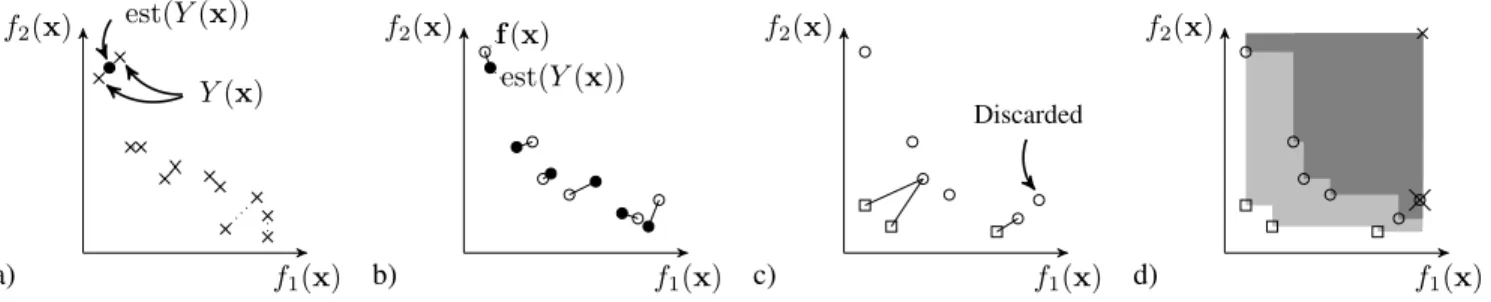
Thequalityof the output of a MOEA is generally difficult to quantify, with different criteria often used to evaluate the non-dominated estimate of the Pareto set produced [36]. In a noisy optimisation, we are concerned with how well the estimated Pareto set matches the actual Pareto set, and also how well the objective values associated with solutions’ est(Y(x)) match their noise-free objective values. Here we use the inverse generational distance and hypervolume measure to quantify how well the estimated non-dominated solutions match the true Pareto set. We also measure the average distance of the objectives associated with designs returned by an optimiser to thetruenoiseless objective values for the designs. We call this measure of quality the noise misinformation (NM) measure. Figure 1 provides an illustration of how these quality measures are calculated.
The noise misinformation measure (see Figure 1b) is the root mean squared Euclidean distance between the best estimate,
est(Y(x)), of the objectives for a particular design and the
2Some MOEAs such as SPEA2 augment the archive with dominated solutions if insufficient non-dominated solutions are available; however, the non-dominated subset from such archives is easy to extract.
f2(x) f1(x) a) est(Y(x)) Y(x) f2(x) f1(x) b) est(Y(x)) f(x) f2(x) f1(x) c) Discarded f2(x) f1(x) d)
Figure 1. Illustrations of the calculation of NM, IGD, and hypervolume in noisy optimisation problems.a)First the estimated objective locations for each xinAneeds to be determined. If there is only a single evaluation perxthen this value is directly used. If multiple samples have been evaluated at each parametrisation (illustrated here with two samples for each archive solution), then these are used to generate theest(Y(x)).b)Illustrates the calculation of the NM measure. Filled circles indicate the estimated Pareto front (est(Y(x))locations) returned by an algorithm. Unfilled circles indicate the actual (noise-free) objective values for eachx. NM is calculated as the root mean squared distance between theest(Y(x))and f(x).c) Illustrates theIGD2 calculation. Unfilled squares indicate samples from the true/noise-free Pareto front and the unfilled circles the noise free evaluations ofA. Solutions which are dominated by other elements ofAin the noise-free evaluation are discarded.IGD2is the root mean squared distance between each member of the true Pareto front which is stored inF and the closest noise-free objectivef(x)forx∈A.d)Illustrates the hypervolume calculation. The region dominated by both the Pareto front and the elements ofAassessed through the non-dominated noise-free evaluationsf(x)forx∈Ais filled with a dark grey, and the region dominated by only the true Pareto frontF is shown in light grey (the reference point used is indicated with the small cross in the top right of the panel). As inc, dominated noise-free evaluations are discarded. The hypervolume is the ratio between the area/volume of the dark grey region and that of the combined dark grey and light grey regions.
noise-free value: NM = 1 |A| X x∈A kest(Y(x))−f(x)k22 !12 . (8) The closer on average the estimated Pareto optimal solutions are to their actual noise-free location, the smaller the NM for a particular algorithm.
If the solutions inAare evaluated using the noise-free objec-tives, the set of objectives associated with the solutions may now contain some dominated solutions. After these dominated solutions have been rejected (see Figure 1c) the proximity and coverage of the estimated Pareto front is also assessed using two widely used quality measures, the inverse generational dis-tance and the hypervolume. Let Fˆ = nondom(f(x)|x∈A), where nondom(E) is the function that returns the maximal set of non-dominated members ofE:
nondom(E) ={u∈E|@(v∈E∧v≺u)}. (9)
We use the power mean version of the inverse generational distance (IGDp) [37], which is not biased by the size of the
estimated Pareto front unlike standard IGD. Given a set F of samples from the true front, this is calculated as:
IGDp( ˆF , F) = 1 |F| X u∈F dist(u,Fˆ)p !1p . (10)
Here the functiondist(u,Fˆ)is the Euclidean distance between uand the closest member ofF, so thatˆ IGDp( ˆF , F)measures
how well on average each sample from the true Pareto front has been approximated by the estimate. As is standard, we use p= 2 in our calculations.
The hypervolume measures the proportion of a given region (defined byF — or a representative subsetF — along with a reference point) that is dominated by both the Pareto frontand
the (noise-free) estimate returned by an MOEA. Unlike the other two measures, the hypervolume is to be maximised. As
with the selection of individuals for assessment inIGDp, the
solutions used fromA in the calculation of the hypervolume are Fˆ, the non-dominated subset when assessed using the noise-free test function (see Figure 1d).
B. Empirical effects
Here we evaluate the effect of different intensities of noise on the performance of four standard (unmodified) MOEAs — PAES, SPEA2, NSGA-II and IBEA+. For these optimisers, therefore, the estimated objective values for a solution are sim-ply a single evaluation of that solution, i.e.est(Y(x))≡y(x). We use the problems UP1-10 from the CEC’09 multi-objective optimisation competition suite [38], and modify them by adding zero-mean isotopic Gaussian noise to each objective, i.e., in (3):d∼ N(0, σ2).
A number of the CEC’09 problems are scalable, and for illustration we use the number of parameters and objectives used in the competition itself [38]. Each MOEA was run 30 times for 300000 function evaluations (as in the competition) for four differentσlevels,σ={0.00,0.01,0.10,1.00}. When σ = 0.00 the objective vector returned for a solution during a run is the true (noiseless) evaluation. The non-dominated members of an unconstrained passive elite archive are recorded for each algorithm every 500 function evaluations; these track the best locations (as perceived in the noisy objective space) that each MOEA has ever visited.
Figures 2 and 3 show the median performance of the algo-rithms using theIGD2and hypervolume measures. It is clear that noise inhibits convergence, and that the effect increases with increasing variance. Even for a very small level of noise, σ= 0.01, the performance of algorithms that previously found solutions in the vicinity of F all degrade. Interestingly one of the problems UP7, behaves slightly differently to the rest: when σ = 0.10 performance of SPEA2 actually improves. A similar effect is seen on UP9 for σ = 0.01. This effect
×IBEA+,4 SPEA2,+NSGA-II, ◦ PAES 10−1 100 101 UP1 IGD 2 10−1 100 UP2 IGD 2 10−1 100 UP3 IGD 2 10−1 100 UP4 IGD 2 10−1 100 101 UP5 IGD 2 10−1 100 101 UP6 IGD 2 100 UP7 IGD 2 10−1 100 101 UP8 IGD 2 100 UP9 IGD 2 0 1 2 3 x 10⁵ 100 101 Evaluations UP10 IGD 2 0 1 2 3 x 10⁵ Evaluations 0 1 2 3 x 10⁵ Evaluations 0 1 2 3 x 10⁵ Evaluations σ= 0.00 σ= 0.01 σ= 0.10 σ= 1.00
Figure 2. Effect of different noise intensities on popular MOEAs on the IGD2 measure. Top to bottom: CEC’09 problems 1-10, Left to right: σ values of{0.00,0.01,0.10,1.00}used. Median results over 30 runs plotted on log scales.
is not peculiar to SPEA2 (as we shall see later, some noise-tolerant optimisers also exhibit this behaviour on UP7), and our conjecture is that the increased diversity in the elite population that results from low levels of noise actually makes UP7 and UP9 easier to search (albeit fordifferentsmall values of noise).
×IBEA+,4SPEA2,+NSGA-II, ◦PAES
0 0.5 1 UP1 Vol. 0 0.5 1 UP2 Vol. 0 0.5 1 UP3 Vol. 0 0.5 1 UP4 Vol. 0 0.5 1 UP5 Vol. 0 0.5 1 UP6 Vol. 0 0.5 1 UP7 Vol. 0 0.5 1 UP8 Vol. 0 0.5 1 UP9 Vol. 0 1 2 3 x 10⁵ 0 0.5 1 Evaluations UP10 Vol. 0 1 2 3 x 10⁵ Evaluations 0 1 2 3 x 10⁵ Evaluations 0 1 2 3 x 10⁵ Evaluations σ= 0.00 σ= 0.01 σ= 0.10 σ= 1.00
Figure 3. Effect of different noise intensities on popular MOEAs on the hypervolume measure. Top to bottom: CEC’09 problems 1-10, Left to right:σ values of{0.00,0.01,0.10,1.00}used. Median results over 30 runs plotted. Reference points used in the hypervolume calculation are (2, 2) and (2, 2, 2), for two-objective and three-objective test problems respectively.
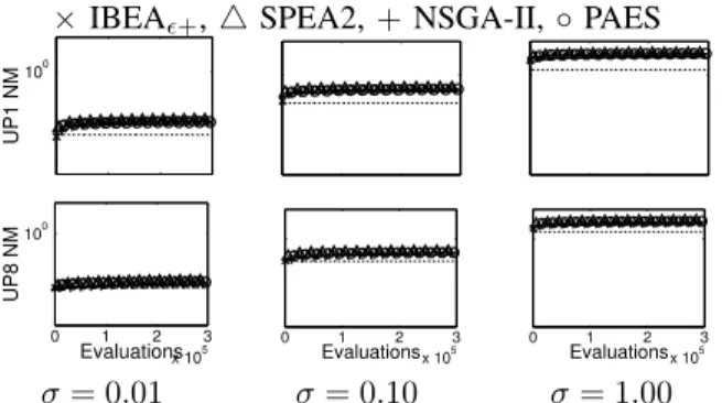
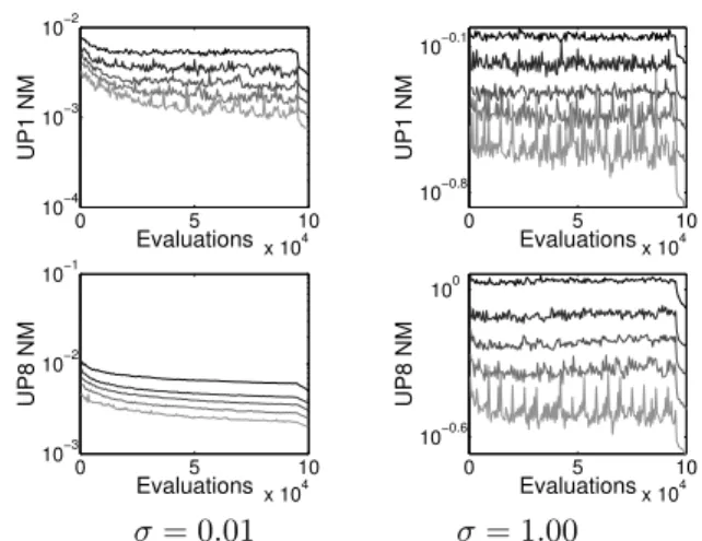
The noise misinformation in the elite solutions for each algorithm is presented in Figure 4. All the results on this measure show a great degree of similarity, so we simply provide plots for UP1 and UP8 (prototypical two and three objective problems). On average, NSGA-II and PAES tend
×IBEA+,4 SPEA2,+NSGA-II, ◦ PAES 100 UP1 NM 0 1 2 3 x 10⁵ 100 Evaluations UP8 NM 0 1 2 3 x 10⁵ Evaluations 0 1 2 3 x 10⁵ Evaluations σ= 0.01 σ= 0.10 σ= 1.00
Figure 4. Effect of different noise intensities on popular MOEAs on the NM measure. Top to bottom: CEC’09 problems UP1,8, Left to right:σvalues of
{0.01,0.10,1.00}used. Median results over 30 runs plotted on log scales. Horizontal dashed lines denote theexpectedNM values if the deviation of passive archived solutions from the noiseless values was unbiased. Note: when σ= 0.00the MN measure is0and so is not plotted.)
to be a little lower, however all algorithms perform in a narrow performance band on this measure. As the optimisation proceeds the NM values can all be seen to rise above the value that would be expected if the solutions were not members of a non-dominated archive. That is, with D objectives it might be anticipated thatN M =√Dσ. In Figure 4 the initial NM is approximately√Dσ, but then rapidly increases above this level. This phenomenon is well-known and is noted in e.g. [16], [17]. In noisy optimisation there are essentiallytwo
drivers pushing the estimated Pareto front forward. The first is (as in noiseless multi-objective optimisation) simply the selection of better solutions. The second driver is the selection of solutions which are affected byoutliernoise [5], [16], [17], that is, noise of large magnitude that makes a solution appear much better than it actually is on one or more objectives. This can rapidly become the main driver for the movement of the estimated front, which quickly becomes filled with those solutions that due to the noise appear to dominate others. This results in the early divergence of the NM measure from the expected value, and highlights the bias introduced by noise which skews the assigned objective values in archives. In this section we have examined the effect of noise on some popular MOEAs, and seen that it causes premature convergence and can exacerbate existing search difficulties for most problem types even with moderate noise. We now briefly look at some of the approaches that have been developed to tackle noisy multi-objective optimisation problems.
IV. NOISE-TOLERANTMOEAS
A number of different avenues have been explored by re-searchers tackling noisy multi-objective optimisation prob-lems. Broadly these can be categorised as those which modify how solutions are compared and stored (as an attempt to prevent ‘bad’ solutions polluting the archive), and those which accept that misleading solutions will exist in the elite set and therefore attempt to reduce the effect of these sub-optimal solutions in the elite population.
The dominance adjustment/redefining approaches almost all
involve resampling at a particular parameter value. Resampling is used to refine the dominance estimation between pairs of solutions, such that the objective quality of a solution is calculated not on a single assessment at a location, but the average over a number of samples. In [5] a fixed number of samples is used and in [21] the number (up to a user-defined maximum) is dynamically varied, based on the estimated variance calculated for a solution; this allows dominance between solutions to be assessed at a particular confidence level prior to assignment to the estimated Pareto subset. The confidence-based dynamic resampling used by [21] is demon-strated to perform favourably compared to basic sampling with a fixed number of samples, fitness inheritance, modified ranking and dominance-dependant lifetime approaches (which are also discussed briefly below) on noisy versions of the ZDT test functions [39]. A variant incorporating a neural network surrogate is also demonstrated on a real world noisy industrial problem. In [6], rather than sample solutions repeatedly until a certain degree of confidence is obtained for a mutually non-dominating set, the probability of dominance is estimated from a fixed number of samples at each design location and used to define an envelope in objective space within which all solutions have a certain probability ofactuallybeing non-dominated (if they were to be evaluated without noise), even though the est(Y(x)) may suggest that some members are dominated. This results in an algorithm which maintains a ‘thick’ elite archive including some suboptimal solutions, but which has a low probability of excluding a solution which would actually be non-dominated without noise. These ap-proaches all build on the work of [13], [14] for the calculation of dominance probabilities. In [7] each solution is modelled as having a probability distribution over objective space, which is estimated by drawing samples at locations and used to estimate the expected indicator function to drive the search process. In [23] the probability of dominance is calculated based on [14] (which assumes the noise is independent on each dimension and Gaussian in nature) and integrated into an estimation of distribution/particle swarm optimisation hybrid algorithm. No resampling is done however, meaning the variance must be known or estimated prior to the optimisation.
In [22] an adaptive number of samples is taken, however unlike [21] the number is not limited. Instead, at each generation all members of a fixed sized archive have additional resam-ples (alongside the resamresam-ples of new locations in the search population). This means that the archive members accumu-late resamples as the search progresses, and, if the archived solution is found to perform worse than originally estimated after additional sampling, it may be removed from the archive. Selection for archive membership is based on (confidence-adjusted) Pareto rank and crowding, and selection for the parent population is based on the ranking and a weighted fitness derived from the number of probabilistically dominated points, reweighted by the number of resamples a solution has (thereby favouring ‘younger’ solutions). Promising results are presented on five of the ZDT problems, when compared to NSGA-II (and noise-tolerant variants thereof).
This does not use resampling, but instead uses a range of other techniques to mitigate the effect of noise, principally experimental learning directed perturbation (which attempts to use learning early on in an optimisation run, when noise tends to have a less detrimental effect on an elite population, in order to learn and exploit ‘good’ directions for perturbations), gene adaptation selection strategy (GASS), which attempts to learn a model of the appropriate area in design space to search, and the use ofpossibilistic archivingwhich uses fuzzy membership functions to limit the size of the archive (which has an effect akin to -dominance [40]). Good results for MOEA-RF are reported in comparison with a range of standard MOEAs, as well as the noise-tolerant SPEA [5] and the multi-objective probabilistic selection evolutionary algorithm (MOPSEA) of [12] on the ZDT test problems corrupted with static noise. In [15] a number of variants of NSGA-II are developed. These include a version which incorporates the probabilistic ranking method of [14], a version which uses resampling to refine the objective location estimate of each solution, and versions where the objective values associated with a new solution are first estimated based upon the mean fitness and noise experienced by its two parents (a form of fitness inheritance), before a decision of whether to resample is taken (this is implemented as an extension of the other approaches). If the observed objectives of the child on evaluation fall within a confidence interval defined by the estimated fitness and noise, then the assigned objective values are accepted, otherwise additional resamples are taken and its fitness is assigned to the mean of these. The performance of these algorithms and standard NSGA-II are compared on noisy ZDT test functions. The resampling approach performing best, with the fitness inheritance variant improving its performance further. In [5] a number of variants of SPEA are presented and compared on test functions with different noise types. In the best performing version non-dominated solutions in the pop-ulation are given a maximum lifespan (in terms of algorithm iterations). The lifespan is inversely proportional to the number of solutions in the general population that a non-dominated solution dominates. That is, if it dominates many, it has a short lifespan, but if it dominates just a few, its lifespan is longer. At the end of its life a solution is removed from the elite set, reevaluated, and its objective values replaced with the new values. The procedure continues as if the reevaluated solution was a newly proposed solution so that a good solution is likely to be included once more into the non-dominated set, but one that experienced outlier noise is likely to be discarded. Results are also presented on the optimisation of a burner in a gas turbine combustion test rig.
The algorithm we now introduce builds on a number of themes in these earlier works. It seeks to minimise the number of algorithm parameters that need tuning and maximise the range of noise types it can be applied to, as well as delivering estimated Pareto optimal solutions which are well converged to F and whose est(Y(x))are highly accurate reflections of f(x).
V. THE ROLLING TIDE EVOLUTIONARY ALGORITHM
In this study we eschew the use of variance learning tech-niques, and instead we focus on the observation that the best estimate for the noise free objectives associated with a design improves with the number of samples taken. Our resultant algorithm is effective not only for static noise, but also time varying and spatially varying noise. As such it can tackle a broader range of problems than many noise-tolerant MOEAs developed so far, with the only a prioriassumption being that an unbiased estimator of the noise-free objectives is available; often this will just be the mean of the noisy evaluations for a particular design. It also does not require additional parameters for e.g. confidence levels, population size, truncation parameters, etc. that are required by other methods, and instead requires the typical parameters of an evolutionary optimiser, such as crossover rate, crossover type, mutation rate and mutation width, plus a variable determining the number of resamples per iteration, and the refinement length at the end of a run.
The algorithm we introduce here repeatedly hones the esti-mated fitness of the stored elite solutions, meaning that the final elite archive solutions have increased accuracy, but not at the cost of reevaluatingalldesigns proposed by the optimiser in its search. This balances the explorative nature of the search with the accuracy of the solutions driving the search forward. The algorithm employs a search populationX, together with an elite archiveA. Decisions on whether to add a solutionx to A are based on the estimated noise-free objective values
est(Y(x)), estimated from a number (possibly 1) of samples Y(x) ={yi(x)}ni=1. In order to gain accurate estimates of the noise free objectives, but to avoid the overhead of reevaluating poor solutions, the algorithm repeatedly reevaluates solutions inA, the leading edge of the estimated Pareto front.
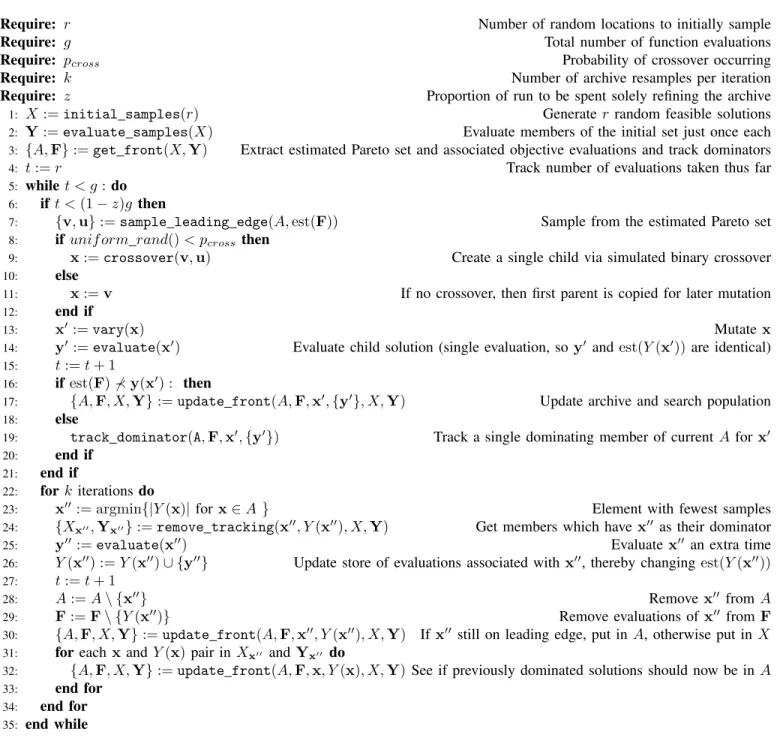
RTEA is outlined in Figure 5. On lines 1-2,rdesign vectors are sampled uniformly in X and each of these is evaluated a single time. We denote by Y the set of sets comprising the objective evaluations; each element of Y is the set of objective evaluations corresponding to a single solution, x. After initialisation each element of Y has a single element corresponding to the single evaluation of a member of X. The non-dominated elite archive is initialised from the initial evaluations (line 3), and extracted from X, meaning that A is the estimated Pareto set, and X contains the solutions evaluated by the algorithm that are not in A. Also, for each member ofX, a single solution whichdominatesit is recorded; this dominating element may be inX or inA.
After initialisation, the algorithm continues in an optimisation loop. During each iteration the algorithm proceeds by assess-ing a new solution in design space (as long as the exclusive refinement phase of the algorithm has not been reached). Two solutions are selected at random from the estimated Pareto set of the solutions evaluated so far (line 7). These solutions are then crossed over with probabilitypcross, using simulated
binary crossover [41], to create a single child (line 9). This child, x, (or clone of an individual parent if no crossover
Require: r Number of random locations to initially sample
Require: g Total number of function evaluations
Require: pcross Probability of crossover occurring
Require: k Number of archive resamples per iteration
Require: z Proportion of run to be spent solely refining the archive
1: X :=initial samples(r) Generate rrandom feasible solutions
2: Y:=evaluate samples(X) Evaluate members of the initial set just once each
3: {A,F}:=get front(X,Y) Extract estimated Pareto set and associated objective evaluations and track dominators
4: t:=r Track number of evaluations taken thus far
5: whilet < g: do 6: ift <(1−z)g then
7: {v,u}:=sample leading edge(A,est(F)) Sample from the estimated Pareto set
8: ifunif orm rand()< pcross then
9: x:=crossover(v,u) Create a single child via simulated binary crossover
10: else
11: x:=v If no crossover, then first parent is copied for later mutation
12: end if
13: x0:=vary(x) Mutatex
14: y0:=evaluate(x0) Evaluate child solution (single evaluation, so y0 andest(Y(x0))are identical)
15: t:=t+ 1
16: ifest(F)6≺y(x0) : then
17: {A,F, X,Y}:=update front(A,F,x0,{y0}, X,Y) Update archive and search population
18: else
19: track dominator(A,F,x0,{y0}) Track a single dominating member of currentA forx0
20: end if
21: end if
22: forkiterationsdo
23: x00:= argmin{|Y(x)|for x∈A} Element with fewest samples
24: {Xx00,Yx00}:=remove tracking(x00, Y(x00), X,Y) Get members which have x00 as their dominator
25: y00:=evaluate(x00) Evaluatex00 an extra time
26: Y(x00) :=Y(x00)∪ {y00} Update store of evaluations associated with x00, thereby changingest(Y(x00))
27: t:=t+ 1
28: A:=A\ {x00} Removex00 fromA
29: F:=F\ {Y(x00)} Remove evaluations ofx00from F
30: {A,F, X,Y}:=update front(A,F,x00, Y(x00), X,Y) Ifx00 still on leading edge, put inA, otherwise put inX
31: foreachx andY(x)pair in Xx00 andYx00 do
32: {A,F, X,Y}:=update front(A,F,x, Y(x), X,Y)See if previously dominated solutions should now be inA
33: end for
34: end for
35: end while
Figure 5. The rolling-tide evolutionary algorithm (RTEA).
occurs) is mutated, creating x0 (line 13). Although we use simulated binary crossover and single element mutation here, other genetic operators could be used.
After its generation, x0 is evaluated once and if it is not dominated by the current estimated Pareto set (based on comparing y0 withest(Y(x)) for x∈ A), it is added to the archive (lines 16 and 17), and any elements in A which are dominated byx0 (based on theirest(Y(x))) are returned toX withx0 recorded as their single trackeddominator. If however x0 is dominated by the estimated Pareto front, then a single member of A is chosen as the single dominator for x0 (line 19), from the members ofAwhich dominatex0. After this, the member of the elite archive with the fewest number of function evaluations,x00, is selected and reevaluated an additional time
(lines 23, 25 and 26). Prior to reevaluation, all solutions inX which have the selected archive memberx00recorded as their single dominator are extracted (line 23); this set is denoted Xx00.
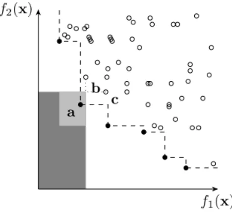
Lines 28-30 ensure that if the reevaluation of x00 means that the solution should no longer be in A, it is removed from A and placed in X. Likewise, lines 31 and 32 ensure that if solutions are no longer dominated by an element of A, they are transferred into A. This may be necessary because, for example, the reevaluated solution’s new est(Y(x00)) means that it now dominates or is dominated by other members of A. An illustration of possible movements of est(Y(x00))and implications for the management of A and X is shown in Figure 6. On line 32 elements which are not inserted intoA
f2(x)
f1(x) a
b c
Figure 6. Potential effects when reevaluating a member ofA. The estimated objective values est(Y(x)) of elements of Aare shown with filled black circles and estimated objective values of elements of X are shown with unfilled circles. The (estimated) attainment surface is plotted with a dashed line. If on reevaluation, the solution markedashifts in itsest(Y(a))position to any location in the light-grey region, AandX will be unchanged. If it moves to any location in the dark-grey region, the membership ofAwill be reduced because it now is estimated to dominate other solutions inA, but there will be no new entrants toAfromX. Movement to any other location will cause band/orcto become non-dominated byAand one or both of them enterAfromX, as well as potentially causing the removal of other members ofA(includingaitself).
remain in X, and a dominating member of A∪Xx00 is set as
their single tracked dominator.
It is thekreevaluations of leading edge solutions each iteration which gives the algorithm its rolling tide name. The effect is to constantly refine the estimate of the leading edge of solutions evaluated thus far. As the search progresses the proposal of new solutions drives the elite archive forward, but the reevaluations pull solutions away from the leading edge (or move them around), leaving others that had previously been dominated to take their place. This differs from e.g. [22], where elite members from the archive may be rejected on reevaluation, but previous solutions are not stored beyond the fixed archive size, and so cannot be pulled back in. The rolling tide approach also has the benefit that although we use a single initial evaluation for search points, the final estimated non-dominated archive tends to have many reevalutions per member and therefore higher confidence in their est(Y(x))
being a good estimate of the underlying true objective values. Finally, RTEA incorporates a refinement phase, in which the search aspect of RTEA is switched off during the final stages of a run, so the algorithm focuses exclusively on increasing the accuracy of the archive. During the refinement phase lines 7-21 are not executed.
A. Efficiently maintaining all evaluations
Since the estimated objectives associated with solutions are uncertain RTEA keeps all solutions that have been evaluated because as solutions are re-evaluated their new estimated objectives may warrant including them in A. As pointed out above, re-evaluation of solutions means that solutions can move back and forth between X and A. Retaining a
large number of solutions inX is potentially computationally expensive because, on the face of it, when a solution in A is reevaluated it has to be compared with all other solutions inAand all those which it previously dominated to discover whether it should still be a member ofA. In practice however the computational overhead may be vastly reduced by main-taining a single reference for each member of X to another member in X or A which dominates it [42]. A member of X need only be compared to A again if its single tracked dominator is the member of A being reevaluated, because if the tracked dominator is not reevaluated, then the tracked dominator solution willstilldominate the member ofX at the current iteration.
In the worst case situation |Xx00| (the number of solutions
which have a resampled member ofA,x00, noted as their single tracked dominator) could equal all the members of X that x00 previously dominated, making the|A| × |Xx00|dominance
comparisons required computationally punitive. However, in practise|Xx00|averages between 3 or 4, as most often the noted
dominator for a solution will end up residing inX (as search progresses) rather thanA. See [42] for complexity derivations and empirical assessments on both synthetic data and optimiser runs.
VI. EMPIRICAL COMPARISON OFRTEAWITH NOISE-TOLERANTMOEAS
In this section we investigate the performance of RTEA and a selection of state-of-the-art noise-tolerant multi-objective optimisers, both for noise whose variance is constant and for noise whose variance varies during the optimisation and over space. The MOEAs compared are:
• The Bayesian (1+1)–ES using probabilistic dominance which we proposed in [6] (labelled BES here).
• The MOEA-RF optimiser of Goh & Tan [16], [17].
• The algorithm of Syberfeldtet al.[21] which is designed to cope with variable noise. We follow the practice of [21] and do not incorporate the optional surrogate which they advise for expensive real-world problems, but do not use in their evaluations on cheap-to-compute test problems. We label the algorithm MOP-EA here.
• The NMOE-AS optimiser of Park & Ryu [22]. • The RTEA optimiser.
As in Section III-B, results are presented on test problems UP1-10 from the CEC’09 test suite [38]. Each algorithm is run 30 times on each of the test problems, for a maximum of 300000 function evaluations. Algorithm parameters used are as suggested by the algorithm proposers [6], [16], [21], [22].3
3For MOEA-RF Goh & Tan recommend repeatedly evaluating a single point to estimate the noise width L at the start of an optimisation. The recommended number of samples is not provided in [16], [17], so here100 samples are used as a reasonable but not excessive number. The values for the reliability thresholdNrandαreweighting term for the crowding distance used in NMOE-AS are not reported in [22], however the values ofNr= 16 andα= 3are used here, after personal correspondence with Dr Park.
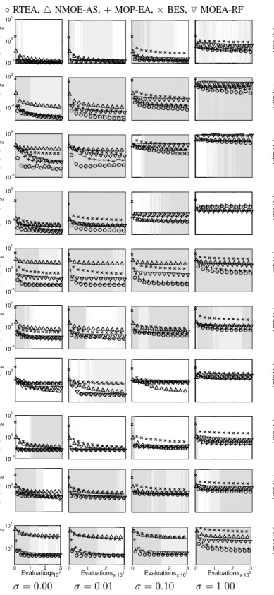
◦RTEA,4NMOE-AS,+MOP-EA,×BES,OMOEA-RF 10−1 100 101 UP1 IGD 2 10−1 100 UP2 IGD 2 10−1 100 UP3 IGD 2 10−1 100 UP4 IGD 2 10−1 100 101 UP5 IGD 2 10−1 100 101 UP6 IGD 2 100 UP7 IGD 2 10−1 100 101 UP8 IGD 2 100 UP9 IGD 2 0 1 2 3 x 10⁵ 100 101 Evaluations UP10 IGD 2 0 1 2 3 x 10⁵ Evaluations 0 1 2 3 x 10⁵ Evaluations 0 1 2 3 x 10⁵ Evaluations σ= 0.00 σ= 0.01 σ= 0.10 σ= 1.00
Figure 7. IGD2 of archived solutions, reevaluated on noiseless cost function on UP1-10; 30 runs, plotted on a log scale. Left to Right: σ =
{0.00,0.01,0.1,1.0}. Top to bottom: UP1-10. A light grey background indicates when the median performance of RTEA is better than all of the other noise-tolerant algorithms, and a darker grey background denotes when it issignificantlybetter.
Here RTEA is started with r= 100 initial random solutions, the mutation probability is set at1/|x|, mutation width =0.2, crossover probability = 0.8, crossover type = SBX, additional
◦RTEA,4NMOE-AS,+MOP-EA,×BES,OMOEA-RF
0 0.5 1 UP1 Vol. 0 0.5 1 UP2 Vol. 0 0.5 1 UP3 Vol. 0 0.5 1 UP4 Vol. 0 0.5 1 UP5 Vol. 0 0.5 1 UP6 Vol. 0 0.5 1 UP7 Vol. 0 0.5 1 UP8 Vol. 0 0.5 1 UP9 Vol. 0 1 2 3 x 10⁵ 0 0.5 1 Evaluations UP10 Vol. 0 1 2 3 x 10⁵ Evaluations 0 1 2 3 x 10⁵ Evaluations 0 1 2 3 x 10⁵ Evaluations σ= 0.00 σ= 0.01 σ= 0.10 σ= 1.00
Figure 8. Hypervolume of archived solutions, reevaluated using the noiseless cost function on UP1-10; 30 runs.Left to Right:σ={0.00,0.01,0.1,1.0}. Top to bottom:UP1-10. Reference points are(2,2)and(2,2,2)for two and three-objective problems respectively. A light grey background indicates when the median performance of RTEA is better than all of the other noise-tolerant algorithms, and a darker grey background denotes when it is significantly better.
resamples per iterationk= 1, refinement phase z= 5% and
A. Static noise
In our first set of experiments we use static Gaussian noise in (3), as used in the experiments with standard MOEAs in Section III-B. We compare the performance of the algorithms for four noise magnitudes: σ ={0.00,0.01,0.10,1.00} and, as before, use the power mean IGD2, the hypervolume and the NM measure to assess the performance of the algorithms. The significance of the comparisons is assessed using the single-tailed non-parametric Mann-Whitney U test at the 5% level. In the plots we present a region with a light grey shading when the median result from RTEA is better than the other noise-tolerant algorithms, and darker grey when it is significantly outperforming all of them, as assessed with paired comparisons using the significance test.
Figure 7 shows the IGD2 results and Figure 8 shows the hypervolume results. RTEA can be seen to be very com-petitive compared to the other noise-tolerant MOEAs when considering the hypervolume, rapidly outperforming the other algorithms across the majority of problems and noise levels, performing better than the other four noise-tolerant MOEAs across problems and noise levels 75% of the time. Assess-ment with the IGD2 measure shows similar performance, with RTEA performing better than the other noise-tolerant MOEAs 71% of the time. On the NM measure, the NMOE-AS algorithm (which also resamples its archive members) tends to do better on the lower noise levels, with RTEA doing better on the higher noise levels, and both outperform the other noise-tolerant algorithms on this measure. Table I compares
all the algorithms across UP1-10 for each noise level, and presents the percentage (averaged across the length of a run) for which the median performance of one algorithm is better (and significantly better) than all the others, averaged across the ten test problems, for each noise level.
It is interesting to note that the ‘standard’ MOEAs actually per-form better than some of the noise-tolerant optimisers, not just in the noiseless case, but also at very low noise levels. In these situations the search/archive populations become slightly more diverse for standard MOEAs, but still hold ‘good’ solutions, meaning the noise-tolerant MOEAs only gain an advantage when the estimated Pareto set is well-converged. Also, many of the noise-tolerant MOEAs were previously assessed only on the ZDT test functions and it is possible that the more difficult UP1-10 problems may demand more sophisticated search and diversity management techniques than they provide. Finally, many all of the noise-tolerant MOEAs expend a substantial proportion of their allotted function evaluations re-evaluating a previously visited location, rather than searching for new samples, which may affect convergence speed. Nevertheless, RTEA is seen to perform better on average on IGD2 when σ ≥ 0.01, and hypervolume when σ ≥ 0.10, although, as mentioned NMOE-AS does better on the NM measure for lowerσ.
Figure 9 shows the median over 30 runs of the NM measure. For those algorithms which resample (RTEA, NMOE-AS, BES and MOP-EA) est(Y(x)) is the mean of the samples at a
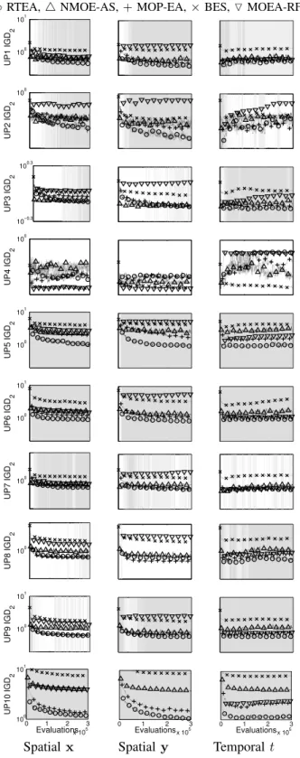
◦RTEA,4NMOE-AS,+MOP-EA,×BES,OMOEA-RF
100 UP1 NM 100 UP2 NM 100 UP3 NM 100 UP4 NM 100 UP5 NM 100 UP6 NM 100 UP7 NM 100 UP8 NM 100 UP9 NM 0 1 2 3 x 10⁵ 100 Evaluations UP10 NM 0 1 2 3 x 10⁵ Evaluations 0 Evaluations1 2 x 1053 σ= 0.01 σ= 0.10 σ= 1.00
Figure 9. NM measure (plotted on the log scale) of archived solutions on noise injected UP1-10; 30 runs.Left to Right:σ={0.01,0.1,1.0}.Top to bottom: UP1-10. A light grey background indicates when the median performance of RTEA is better than all of the other noise-tolerant algorithms, and a darker grey background denotes when it issignificantlybetter.
locationx. We note that for MOEA-RF, which makes only a single evaluation at each design, est(Y(x)) = y. NMOEA-AS and RTEA can be seen to improve the measure as the search continues. In contrast, for a number of problems the other algorithms become worse according to NM as search progresses. Note also the effect of the final 5% of the RTEA runs: when searching is discontinued and the archive further refined with resamples it is clear from Figure 9 that the
Table I
PERCENTAGE OF TOTAL RUN LENGTH THAT THE MEDIAN PERFORMANCE OF EACH ALGORITHM WAS BETTER THAN THE OTHER EIGHT,AVERAGED OVER
UP1-10,ON STATIC NOISE TYPES WITHσ={0.00,0.01,0.10.1.00}. PERCENTAGE SIGNIFICANTLY BETTER GIVEN IN PARENTHESIS. BOLD INDICATES
LARGEST PERCENTAGE. VALUES ROUNDED TO NEAREST WHOLE NUMBER.
Hypervolume IGD2 NM σ 0.00 0.01 0.10 1.00 0.00 0.01 0.10 1.00 0.00 0.01 0.10 1.00 RTEA 17 (10) 32 (24) 56(48) 53(37) 10 (4) 46(28) 73(51) 56(41) - 19 (16) 15(12) 77(69) MOP-EA 0 (0) 0 (0) 1 (0) 12 (9) 8 (2) 0 (0) 6 (4) 18 (9) - 0 (0) 0 (0) 0 (0) BES 0 (0) 0 (0) 0 (0) 4 (0) 8 (0) 0 (0) 0 (0) 3 (0) - 1 (1) 1 (1) 2 (1) MOEA-RF 9 (1) 6 (0) 0 (0) 1 (0) 3 (0) 3 (0) 0 (0) 7 (2) - 0 (0) 0 (0) 0 (0) NMOE-AS 0 (0) 0 (0) 23 (4) 3 (0) 6 (0) 2 (1) 19 (10) 1 (0) - 79(77) 84(81) 21 (18) IBEA+ 31 (6) 13 (2) 9 (2) 12 (2) 11 (0) 4 (0) 2 (0) 9 (2) - 0 (0) 0 (0) 0 (0) SPEA2 38(23) 49(20) 1 (0) 2 (0) 53(50) 45 (23) 1 (0) 6 (0) - 0 (0) 0 (0) 0 (0) NSGA-II 3 (0) 0 (0) 14 (9) 12 (10) 0 (0) 0 (0) 0 (0) 0 (0) - 0 (0) 0 (0) 0 (0) PAES 1 (1) 0 (0) 0 (0) 0 (0) 2 (1) 0 (0) 0 (0) 0 (0) - 0 (0) 0 (0) 0 (0) Table II
PERCENTAGE OF TOTAL RUN LENGTH THAT THE MEDIAN PERFORMANCE OF EACH ALGORITHM WAS BETTER THAN THE OTHER EIGHT,AVERAGED OVER
UP1-10,ON VARIABLE NOISE TYPES. PERCENTAGE SIGNIFICANTLY BETTER GIVEN IN PARENTHESIS. BOLD INDICATES LARGEST PERCENTAGE. VALUES
ROUNDED TO NEAREST WHOLE NUMBER.
Hypervolume IGD2 NM Noise type y x t y x t y x t RTEA 45(28) 54(40) 49(26) 62(45) 70(57) 60(38) 12 (11) 31 (31) 4 (3) MOP-EA 15 (3) 10 (9) 0 (0) 12 (3) 11 (9) 0 (0) 25 (20) 34(28) 4 (0) BES 1 (0) 0 (0) 0 (0) 5 (0) 0 (0) 10 (10) 0 (0) 0 (0) 1 (0) MOEA-RF 0 (0) 0 (0) 0 (0) 5 (1) 0 (0) 0 (0) 0 (0) 0 (0) 0 (0) NMOE-AS 33 (23) 35 (26) 14 (7) 2 (1) 8 (3) 0 (0) 6 (1) 14 (8) 0 (0) IBEA+ 4 (0) 0 (0) 10 (0) 10 (3) 0 (0) 6 (0) 0 (0) 0 (0) 0 (0) SPEA2 1 (0) 0 (0) 17 (0) 1 (0) 0 (0) 24 (0) 39(24) 0 (0) 75(69) NSGA-II 2 (0) 1 (0) 10 (9) 3 (0) 10 (10) 0 (0) 18 (0) 20 (20) 20 (20) PAES 0 (0) 0 (0) 0 (0) 0 (0) 0 (0) 0 (0) 0 (0) 0 (0) 0 (0)
NM measure decreases sharply in this final phase of the optimisation run. Nonetheless, even in the general search (during the first 95% of the optimisation) the discrepancy between the true objectives and the estimated objectives is smaller for RTEA than other algorithms, bar NMOEA-AS, due to its iterative re-estimation of the leading part of the front. These more accurate estimates of the front’s location in turn allow faster convergence towards the true front.
B. Variable noise
In the previous experiments the noise was static. We now investigate the effect of different forms of noise which varies with objective space location or the duration of the optimi-sation. We modify the CEC’09 test functions to have noisy objectives, via (3), in three ways. First, the noise variance depends on the objective space location of the solution: d ∼ N(0, fd(x)). Second, the noise depends on the design
space location of the solution: d ∼ N
0,(0.1||x||1)2
. Of course, noise that varies with design space location can be regarded as a function of objective space location and vice versa. Nonetheless, the quality of the noise variation will be different and, in general, noise that varies as a function of design space is likely to vary more rapidly in objective space than noise that is a function of objective values. Finally, the noise is made temporally dependent noise: d ∼ N(0, ωd,t2 ),
where ωd,t is generated via a filtered random walk for each
objective independently, with t denoting the time step of the walk. ωd,t is generated according to the following nonlinear
autoregressive process: ωd,t= ( 0.1, ift= 1 |ωd,t−1+ξd|, otherwise (11)
with ξd ∼ N(0,0.012). In the case of temporal noise, we
generate a single set of 30 random walks using (11), and use these 30 for each algorithm so that each algorithm encounters the same temporal noise as its comparators.
The BES algorithm incorporates a termη which progressively down-weights the influence of historically observed noise in the Bayesian update scheme in order to cope withtemporally
varying noise [6]. We can also apply BES to the spatially-varying noise problems, because, since BES is a point-based optimiser, spatially varying noise is equivalent to temporally varying noise, although with high frequency variations. We useη= 0.95here for the temporally varying noise and for the noise dependent on objective space location, andη= 0.75for the noise dependent on design space location which changes more rapidly.
Since MOP-EA and NMOE-AS continuously re-estimate the noise by resampling, they can also be applied to situations where the noise varies spatially, as they effectively maintain a noise estimate at each design space location. Although a stationary, zero mean, Gaussian distributed model is no longer accurate, [21] still recommends its use when the noise is non-Gaussian, although the accuracy of the estimated confidence intervals will be affected. We therefore also apply it to the temporally varying noise problem. [22] adjusts the probability
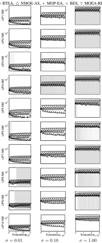
◦RTEA,4NMOE-AS,+MOP-EA,×BES,OMOEA-RF 100 101 UP1 IGD 2 100 UP2 IGD 2 10−0.3 100.3 UP3 IGD 2 100 UP4 IGD 2 100 101 UP5 IGD 2 100 101 UP6 IGD 2 100 UP7 IGD 2 100 UP8 IGD 2 100 101 UP9 IGD 2 0 1 2 3 x 10⁵ 100 101 Evaluations UP10 IGD 2 0 1 2 3 x 10⁵ Evaluations 0 1 2 3 x 10⁵ Evaluations
Spatialx Spatialy Temporalt
Figure 10. IGD2 of archived solutions on varying noise problems, reeval-uated on noiseless cost function on UP1-10; 30 runs, plotted on a log scale. Left to Right:Spatialx, spatialy, temporal.Top to bottom:UP1-10. A light grey background indicates when the median performance of RTEA is better than all of the other noise-tolerant algorithms, and a darker grey background denotes when it issignificantlybetter.
of dominance calculation when the noise variance is assumed to vary at different locations.
Like a number of noise-tolerant optimisers, MOEA-RF is
◦RTEA,4NMOE-AS,+MOP-EA,×BES,OMOEA-RF
0 0.5 1 UP1 Vol. 0 0.5 1 UP2 Vol. 0 0.5 1 UP3 Vol. 0 0.5 1 UP4 Vol. 0 0.5 1 UP5 Vol. 0 0.5 1 UP6 Vol. 0 0.5 1 UP7 Vol. 0 0.5 1 UP8 Vol. 0 0.5 1 UP9 Vol. 0 1 2 3 x 10⁵ 0 0.5 1 Evaluations UP10 Vol. 0 1 2 3 x 10⁵ Evaluations 0 1 2 3 x 10⁵ Evaluations
Spatialx Spatialy Temporalt
Figure 11. Hypervolume of archived solutions on varying noise problems, reevaluated on noiseless cost function on UP1-10; 30 runs.Left to Right: Spatialx, spatialy, temporal.Top to bottom:UP1-10. Reference points used in the hypervolume calculation are (2, 2) and (2, 2, 2), for two-objective and three-objective test problems respectively. A light grey background indicates when the median performance of RTEA is better than all of the other noise-tolerant algorithms, and a darker grey background denotes when it is significantlybetter.
designed for situations with a fixed noise width and requires the noise variance to be specified as a parameter of the
0 5 10 x 104 10−0.9 10−0.1 Evaluations UP1 IGD 2 0 5 10 x 104 10−0.5 100 Evaluations UP1 IGD 2 0 5 10 x 104 100 Evaluations UP8 IGD 2 0 5 10 x 104 100 Evaluations UP8 IGD 2 σ= 0.01 σ= 1.00
Figure 12. IGD2 of RTEA with k = {1,2,3,5,10}. UP1, UP8, σ =
{0.01,1.00}. 0 5 10 x 104 0.2 0.4 0.6 0.8 1 Evaluations UP1 Hypervolume 0 5 10 x 104 0 0.2 0.4 0.6 0.8 Evaluations UP1 Hypervolume 0 5 10 x 104 0 0.5 1 Evaluations UP8 Hypervolume 0 5 10 x 104 0 0.2 0.4 0.6 0.8 Evaluations UP8 Hypervolume σ= 0.01 σ= 1.00
Figure 13. Hypervolume of RTEA withk = {1,2,3,5,10}. UP1, UP8, σ={0.01,1.00}.
algorithm. Consequently we anticipate that the algorithm will perform relatively poorly on varying noise problems, however we include the results here for completeness.
Figures 10 and 11 show the results using the IGD2 and hypervolume. A similar ordering of algorithms is seen as with the static noise, with RTEA performing better than the other four noise-tolerant MOEAs across problems and noise types on the hypervolume measure 58% of the time; and on the IGD2 measure 73% of the time.
Table II compares allthe algorithms across UP1-10 for each type of variable noise. When the noise varies according to y or x RTEA and NMOE-AS perform better than all other algorithms on the hypervolume measure, although RTEA tends to do much better on IGD2than NMOE-AS. When the noise varies over time NMOE-AS performs markedly less well, although it remains in second place. The NM measure is not well-correlated with the other two quality measures on variable noise, but this is unsurprising — for many of the problems the closer solutions are to the Pareto set (or sub regions thereof) the larger the noise intensity they experience, and therefore the higher the NM that would be expected.
0 5 10 x 104 10−4 10−3 10−2 Evaluations UP1 NM 0 5 10 x 104 10−0.8 10−0.1 Evaluations UP1 NM 0 5 10 x 104 10−3 10−2 10−1 Evaluations UP8 NM 0 5 10 x 104 10−0.6 100 Evaluations UP8 NM σ= 0.01 σ= 1.00
Figure 14. NM of RTEA with k = {1,2,3,5,10}. UP1, UP8, σ =
{0.01,1.00}. 0 5 10 x 104 0 200 400 600 Evaluations
UP1 Av. resamps
0 5 10 x 104 0 100 200 300 400 Evaluations
UP1 Av. resamps
0 5 10 x 104 0 50 100 Evaluations
UP8 Av. resamps
0 5 10 x 104 0 50 100 150 200 Evaluations
UP8 Av. resamps
σ= 0.01 σ= 1.00
Figure 15. Average number of resamples of archive members in RTEA with k={1,2,3,5,10}. UP1, UP8,σ={0.01,1.00}.
C. Sensitivity analysis of RTEA
The lower the number of k resamples of archive members taken at each iteration, the more evaluations are available to RTEA for searching new locations (given a limited number of total function evaluations). But the archived solutions, from which the new solutions are evolved, will have estimated ob-jective values of lower accuracy. Here we perform a sensitivity analysis of RTEA with various numbers of resamples taken of archive members at each iteration. We run RTEA 30 times for 100000 function evaluations on the two-objective CEC’09 problem UP1 and the three-objective CEC’09 problem UP8, with k = {1,2,3,5,10}. The corresponding median IGD2, hypervolume and NM measure results of these experiments are shown in Figures 12-14, and the median number of resamples per archive member is shown in Figure 15, for σ={0.01,1.0}. The greyscale of the lines plotted correspond to the value ofk, withk = 1 drawn with black andk = 10
with the lightest grey.
When the noise level is small, RTEA with lower k performs better than with higher k on IGD2 and hypervolume. NM is always lower with higher k, irrespective of the noise level – this is as expected, because the largerk, the more resamples
(on average) an archived solution will have (see Figure 15), and therefore the more accurate the est(Y). For the large noise level smaller k performs better initially on IGD2 and hypervolume, but is then rapidly overtaken by the RTEA algorithms using largerk. Based on these observations, there is potential in to developing a variant of RTEA in which k is adapted during the search, based on the noise properties encountered. However, as seen here, even with k= 1, RTEA performs competitively with other state-of-the-art approaches.
VII. DISCUSSION
In this paper we have presented a novel algorithm for multi-objective optimisation with uncertain multi-objectives, the rolling tide evolutionary algorithm (RTEA). RTEA can cope with noisy optimisation problems in which the noise characteristics may be fixed or variable. We make the minimal assumption that the noiseless objectives can be accurately estimated from a sufficiently large number of samples. The algorithm attempts to both harness the exploitation/exploration power of tradi-tional EAs, whist simultaneously refining the accuracy of its active elite archive by constantly resampling the elite solutions, thus ensuring that ‘high-quality’ individuals feed into the evolutionary process. The approach also means that solutions are not ‘lost’ if another solution is thought to dominate them initially, but on reevaluation this is found to perform less well, thus allowing previously dominated solutions to be pulled into the archive at a later time step. If the algorithm is run with a single reevalution each iteration, roughly half of all function evaluations are at new locations and half are used in the reevaluation of previously evaluated locations, allowing RTEA to search to a much greater extent than most other noise-tolerant MOEAs.
We have shown that for even small values of noise the performance of standard MOEAs is significantly impaired, and we have also shown the ability of RTEA to cope well with noisy optimisation problems in comparison to a number of state-of-the-art noise-tolerant MOEAs. RTEA produces competitive results with state-of-the-art algorithms on a range of problem types, noise types and intensities. We find the next best competing algorithm is NMOE-AS, which like RTEA progressively resamples its archive (although without the ability to pull in previously dominated solutions to its archive). Progressive resampling therefore appears to be a very useful technique for noise-tolerant MOEAs
RTEA is simple to implement and also has the benefit of requiring relatively few parameters. It does rely on keeping all previously evaluated solutions (which has a storage overhead), however we have also discussed a method to ameliorate the cost associated with updating the elite archive in conjunction with these past solutions, based on tracking just a single dom-inating solution for each member of the non-elite population. A potential extension of RTEA would be an automatic pro-cedure for determining when to resample. Currently at each iteration a new location is evaluated and existing estimated elite solution(s) reevaluated. By tracking, for instance, the
region dominated by the elite estimate over time the ratio of new location evaluations and resamples could be beneficially varied. When the elite front is advancing more new designs could be evaluated, whereas if the front is stalled or oscillating (due to reevaluations pulling the estimate back), then more resamples may be preferred. This would allow the algorithm to tune itself to different problem types and convergence stages. Although RTEA has shown good performance on spatially varying noise, we believe there is still scope to improve performance on these types of problems further, by learning
the spatially dependent characteristics of the noise during the search using, for instance, machine learning methods [10]. We look forward to the development of more sophisticated algorithms that can take advantage of learned characteristics to reduce the number of function evaluations required.
REFERENCES
[1] I. Rechenberg, “Evolutionsstrategie – optimierung technischer systeme nach prinzipien der biologischen evolution,” Ph.D. dissertation, Techni-cal University of Berlin, Federal Republic of Germany, 1971. [2] A. Thompson, “Hardware evolution: Automatic design of electronic
circuits in reconfigurable hardware by artificial evolution,” Springer, 1998.
[3] S. Harding and J. F. Miller, “Evolutionin materio: initial experiments with liquid crystal,” in Proceedings of the NASA/DoD Workshop on Evolvable Hardware. IEEE Computer Society, 2004, pp. 289–299. [4] P. Stagge, “Averaging Efficiently in the Presence of Noise,” inParallel
Problem Solving from Nature, A. Eiben, T. B¨ack, M. Schoenauer, and H.-P. Schwefel, Eds. Springer, 1998, pp. 188–200.
[5] D. B¨uche, P. Stoll, R. Dornberger, and P. Koumoutsakos, “Multiobjective evolutionary algorithm for optimization of noisy combustion processes,” IEEE Transactions on Systems, Man, and Cybernetics – Part C: Appli-cations and Reviews, vol. 32, no. 4, pp. 460–473, 2002.
[6] J. Fieldsend and R. Everson, “Multi-objective optimisation in the pres-ence of uncertainty,” inIEEE Congress on Evolutionary Computation, 2005, pp. 243–250.
[7] M. Basseur and E. Zitzler, “A preliminary study on handling uncertainty in indicator-based multiobjective optimization,” inApplications of Evo-lutionary Computation. EvoWorkshops 2006: EvoBIO, EvoCOMNET,
EvoHOT, EvoIASP, EvoINTERACTION, EvoMUSART, and EvoSTOC,
ser. LNCS, vol. 3907. Springer, 2006, pp. 727–739.
[8] S. Rana, L. Whitley, and R. Cogswell, “Searching in the Presence of Noise,” in Parallel Problem Solving from Nature. Springer Verlag, 1996, pp. 198–207.
[9] A. Di Pietro, L. While, and L. Barone, “Applying Evolutionary Algo-rithms to Problems with Noisy, Time-consuming Fitness Functions,” in IEEE Congress on Evolutionary Computation, vol. 2. IEEE, 2004, pp. 1254–1261.
[10] Y. Jin and J. Branke, “Evolutionary optimization in uncertain environments-a survey,”IEEE Transactions on Evolutionary Computa-tion, vol. 9, no. 3, pp. 303–317, 2005.
[11] J. Horn and N. Nafpliotis, “Multiobjective Optimization Using the Niched Pareto Genetic Algorithm,” Illinois Genetic Algorithms Labora-tory (IlliGAL), University of Illinois at Urbana-Champaign, USA, Tech. Rep. 93005, July 1993.
[12] E. Hughes, “Constraint handling with uncertain and noisy multi-objective evolution,” in IEEE Congress on Evolutionary Computation, 2001, pp. 963–970.