Valuing Environmental Quality: A Space-based
Strategy
John I. Carruthers ✩
U.S. Department of Housing and Urban Development, Office of Policy Development and Research; University of Washington, Department of Urban Design and Planning; University of Maryland, National Center for Smart Growth Research and Education (e-mail:
David E. Clark
Marquette University, Department of Economics (e-mail: [email protected])
✩ Corresponding author.
U.S. Department of Housing and Urban Development working paper # REP 07-01
This paper and related research have been presented at the 2007 meetings of the Southern Regional Science Association in Charleston, South Carolina; the 2007 meetings of the European Regional Science Association in Paris, France; the 2007 meetings of the North American Regional Science Council in Savannah, Georgia, and at a seminar at the University of Maryland. Special thanks to session participants for their helpful comments and feedback and, also, to Robert Renner for his invaluable research assistance. Some of the work on this project was conducted while John Carruthers was the Director of Research at Greenfield Advisors, and the firm’s support is gratefully acknowledged. The opinions expressed in this paper are those of the authors and do not necessarily reflect the opinions of the Department of Housing and Urban Development or the U.S. government at large.
This paper develops and applies a space-based strategy for overcoming the general problem of getting at the demand for non-market goods. It focuses specifically on evaluating one form of environmental quality, distance from EPA designated environmental hazards, via the single-family housing market in the Puget Sound region of Washington State. A spatial two stage hedonic price analysis is used to: (1) estimate the marginal implicit price of distance from air release sites, hazardous waste generators, hazardous waste handlers, superfund sites, and toxic release sites; and (2) estimate a series of demand functions describing the relationship between the price of distance and the quantity consumed. The analysis, which represents a major step forward in the valuation of environmental quality, reveals that the information needed to identify second-stage demand functions is hidden right in plain site — hanging in the aether of the regional housing market.
1. Introduction
The research presented in this paper is motivated by the need to better understand the value of environmental quality. Over the last several decades, the demand for that commodity has emerged as one of the most powerful forces acting on the economic landscape of the United States and other developed nations (see Kahn 2006). Viewed among regions, the influence of relative living conditions is so strong that they are observed to direct migration flows and generate compensating differentials in labor and housing markets. Viewed within a single region, environmental quality is similarly observed to affect where households choose to live and the price they pay in the housing market to realize that choice. While the two forms of influence play out across different levels of geography, they are closely connected and they each involve the identical set of mechanisms: (1) households compete to occupy environmentally desirable locations; and (2) in order to secure the right to do so, they incur costs that depend directly upon the comparative appeal of the spot in question. Through these actions, the place-to-place variation in environmental quality has become a main organizing force within the American space economy.
But, in spite of its great importance, the value of environmental quality remains elusive because complete measurement requires knowledge of a demand function that describes the relationship between price and the quantity consumed. The challenges that this presents are several. To begin with, environmental quality is spatial in nature, so its mechanism of economic influence needs to be conceptualized and, ultimately, expressed in that way. Moreover, no conventional market for environmental quality exists, so, once it is measured, it can only be valued indirectly — ideally, via preferences revealed in markets for larger, differentiated commodities, like housing. Although it is usually straightforward to estimate the marginal implicit prices of the various non-market goods embedded in such markets, the function used to do this, called a hedonic price function, is a market clearing function that results from interaction between the bid and offer functions of participants on either side of the market (Rosen 1974). Recovering the prices of non-marginal differences in consumption, which are needed for welfare analysis, means extending hedonic price analysis to a second stage and estimating a demand function wherein price and quantity are endogenously determined. The problem is that, because the underlying first stage function is a composite of both demand and supply, conventional econometric procedures cannot readily be used to identify the demand function the way they can for more traditional commodities. Each of these issues makes it hard to evaluate environmental quality in a holistic way.
This paper responds to the challenge with an analysis that leverages spatial non-stationarity in housing attribute prices to expose the demand for one aspect of environmental quality, distance from Environmental Protection Agency (EPA) designated environmental hazards. There are three specific research objectives: (1) to define spatial non-stationarity in the context of housing markets and develop a strategy for using it to overcome the general problem of getting at the demand for non-market goods; (2) to estimate the marginal implicit price of distance from air release sites, hazardous waste generators, hazardous waste handlers, superfund sites, and toxic release sites via the single-family housing market in the Puget Sound region of Washington State; and (3) to estimate a series of demand functions describing the relationship between the price of distance from environmental hazards and the quantity consumed. The analysis represents a major step forward in valuing environmental quality and, as important, it reveals how the field of regional science’s unifying epistemology — namely, that geographic space mediates socioeconomic processes — holds a workable solution to what has always been the albatross of two stage hedonic price analysis.
2. Background Discussion
2.1 Hedonic Prices and Implicit Markets
Environmental quality is not traded in conventional markets so willingness to pay for it can only be estimated, never measured directly. Estimation is done either via stated preference approaches, such as contingent valuation, or via revealed preference approaches, such as hedonic price analysis (see Freeman 2003 for a more detailed description of the material presented in this and the next several paragraphs). In the latter case, competition for the right to occupy desirable locations — both among and within regions — generates implicit prices in labor and/or housing markets that correspond to spatial variation in environmental quality. And, since this process plays out across two different levels of geography, there are two corresponding levels of hedonic price analysis: (1) interregional analysis, which deals with variation in wages (the price of labor) and housing prices among regions; and (2) intraregional analysis, which deals with variation in housing prices within regions.1 Although the theory underpinning these two frameworks is
essentially the same, the distinction is an important one because the appropriate lens depends on the nature of the environmental commodity in question. For example, the value of sunshine is best measured by looking among regions and, conversely, the value of proximity to neighborhood parks is best evaluated by looking within regions. Though both levels of analysis have long been
1 See Carruthers and Mundy (2006) for a broad survey of the two levels of hedonic price analysis.
€ € € € € € € € €
used to evaluate environmental hazards, it is the intraregional level of analysis that is the focus of this paper.
Rosen (1974) originally formalized hedonic price analysis, which may be used to disaggregate the price of housing — or any other differentiated commodity, like labor — into its component parts, as a two-stage process. In the first stage, the transacted price is regressed on measures of all of the things that matter to it, including structural features, neighborhood characteristics, and environmental factors that vary by location. This stage estimates the hedonic price function, and it contains a vector of parameters giving the marginal implicit price of each attribute. Then, in the second stage, quantities of the attributes of interest are regressed on their estimated marginal implicit prices, which are endogenous, a set of exogenous demand shifters, and the prices of relevant complements and/or substitutes. This stage generates the demand function, and it is needed for recovering the values of non-marginal differences in the quantity consumed and for estimating assorted elasticities of demand.
In the language of hedonic price theory, housing is described as a bundle of k attributes contained in a vector z, where z= (z1, z2, ...,zk), so its equilibrium price, p(z), is a function of each of those attributes: p(z)= p(z1, z2, ...,zk). This function, which corresponds to the first stage of the process just described, develops as long as: (1) there is perfect information about the bundle; (2) there are no costs associated with trading it; and (3) there is a continual offering of its attributes in the housing market. As shown in Figure 1, the hedonic price function is a market clearing function that emerges as a result of the interaction between the bid functions of consumers (b1, b2, b3) and the offer functions of producers (o1, o2, o3). The figure also illustrates
that the function is normally assumed to be nonlinear, and this is because it is not practical to repackage or otherwise arbitrage a bundle of housing attributes. The reason for this is that a household cannot simultaneously consume the floor area of one home, the neighborhood of another, and the view of yet another — no matter how much happiness it would gain from such an arrangement. Under these assumptions, the marginal implicit price of any given attribute, zk, is defined as the partial derivative of the hedonic price function with respect to that attribute, or
pz
k(z)= ∂p/∂zk.
The values of these marginal implicit prices are estimated in the first stage of hedonic price analysis:
p˜i = α0 +α1 ⋅zi1 +α2 ⋅zi2 + ...+αk ⋅zik +εi . (1)
In this equation, p˜i represents the natural log of the sales price of home i; the zs represent measures of housing attributes; the αs represent estimable parameters; and εi represents a
€ € € € € € € € € € € € € € € € € € € € € € € € € € €
stochastic error term. From this, the marginal implicit price of any attribute, k, for each home, i, is calculated as the product of the estimated parameter and the price of the home, or πˆik= αˆk⋅pi,2
and the total implicit expenditure is calculated as the product of the marginal implicit price and the quantity of that attribute, or ηˆik= πˆik⋅zik
Before discussing the second stage, note that information about environmental quality may not be perfect and, so, in practice, its impact on the hedonic price function depends on how much is known about it (Clark and Allison 1999). To see this, suppose that there is an index of public knowledge, κ, about an environmental hazard that ranges between zero (no information) and one (perfect information). With this index in the mix, the hedonic price function depends on the perceived level of the hazard, not the actual level of the hazard: ˙˙˙z = f (z, κ) is not necessarily equivalent to z. So, pz is instead p˙˙˙z (z) = ∂p /∂˙˙˙z , which means that, if κ= 0, ˙˙˙z = f (z, 0) = 0 and,
if κ= 1, ˙˙˙z = f (z,1) = z . Anywhere along this continuum, the implicit price, p˙˙˙z , is a function of
both the actual level of the environmental hazard in question, z, and the level of information associated with it, κ. And, because distance, d, decreases both the actual level of the hazard and the level of information about it, in most instances, the perceived level declines with separation. With this added wrinkle, the marginal implicit price of distance is something more complicated than just ∂p/∂z, the straight partial derivative that measures most other implicit prices.3 Rather, it
is expressed as: ∂p(˙˙˙z (z,κ)) /∂d = ∂p /∂˙˙˙z ⋅∂˙˙˙z /∂z ⋅∂z /∂d +∂p /∂˙˙˙z ⋅∂˙˙˙z /∂κ⋅∂κ/∂d . No matter what, the influence of distance is expected to be positive because both terms on the right-hand side of this extended partial derivative are expected to be positive. In the case of the first term, ∂p /∂˙˙˙z < 0, ∂˙˙˙z /∂z > 0, and ∂z/∂d< 0, so their product is positive; likewise, in the case of the second term, ∂p /∂˙˙˙z < 0, ∂˙˙˙z /∂κ> 0, and ∂κ/∂d< 0 so their product is positive. While it adds additional complexity, this expression captures the exact mechanism that causes distance from environmental hazards to positively influence the price of housing.
Moving on, Rosen’s (1974) formalization of hedonic price analysis suggested that the endogeneity between price and quantity in the second stage amounted to a “garden variety identification problem” (page 50). Unfortunately, as demonstrated by Brown and Rosen (1982), the situation is not so simple because, in hedonic price analysis, each revealed implicit price function results from a unique interaction between an individual demand function and an
2 Because equation (1) in semi-log form, marginal implicit price is αˆ
k⋅ pi; if equation (1) were linear, the implicit price
would be just αˆ k; and, if it were in log-log form, the marginal implicit price would be αˆk⋅ pi/ zi. The calculations that come later in the paper account for the log transform of the dependent variable and, where appropriate, explanator variables.
3 For the sake of clarity, the notation used in this paragraph applies to a simple linear relationship — that is, one where
αˆk= ∂p/∂z gives the marginal implicit price.
€ € € € € € € €
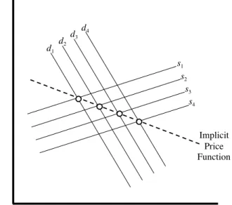
individual supply function. As shown in Figure 2, the implicit price function is, like the hedonic price function it comes from, a reduced form composite of both demand (d1, d2, d3, d4) and supply
(s1, s2, s3, s4) so it alone does not contain the information needed to identify the second-stage
function. Though there are multiple ways of overcoming this problem, the most widely accepted strategy is to use spatially distinct housing market segments having different prices for the same attributes to identify a demand function for the entire market (Brown and Rosen 1982; Palmquist 1984; Bartik 1987; Epple 1987). While the parameter estimates of the resulting demand functions are spatially invariant, it is the spatial variation in the underlying marginal implicit price estimates that are critical to identifying the demand function.
So, in the second stage of a hedonic price analysis, estimated marginal implicit prices from different locations are pooled to estimate a single demand function describing the relationship between price and quantity:
q˜ik = β0 +δik ⋅πˆik + β1 ⋅xi1 + ...+ βs ⋅xis +υi . (2)
Here, q˜ik represents the natural log of the quantity of attribute k consumed via home i; πˆik represents its estimated marginal implicit price; the x s represent s number of demand shifters, plus the prices of relevant complements and/or substitutes; δik the βs represent estimable parameters; and υi represents a stochastic error term. Because this equation contains an
endogenous variable ( πˆik) it must be estimated via an instrumental variables procedure, like two stage least squares (2SLS). Once this is accomplished, the resulting demand function can be used to look at the price and income elasticities of demand, cross-price elasticities, and many other objects of interest.
Over the years, variations on the first stage of hedonic price analysis have been used to examine many general forms of environmental quality (see Boyle and Kiel 2001 and Kiel 2006 for reviews), plus a number of specific environmental hazards (for example, Kohlhase 1991; Kiel and McClain 1995; Clark et al. 1997; Clark and Allison 1999; Hite et al. 2001). And, recently, there has been a revived interest in the second stage of hedonic price analysis, which has been used to evaluate the demand for air quality (Chattopadhyay 1999; Zabel and Kiel 2000), neighborhood and school quality (Cheshire and Sheppard 1995, 1998, 2004; Brasington 2000, 2003); and distance from environmental hazards similar to those that are of concern here (Brasington and Hite 2005). In addition to the growing commitment to second stage analysis, there have been important advances in first stage analysis, including those made by a number of recent studies that use spatial econometric methods to evaluate various forms of environmental quality (Kim et al. 2003; Theebe 2004; Anselin and LeGallo 2006). Still other spatial econometric analyses — beginning with work by Can (1990, 1992) — have revealed that there is a high
€ €
degree of spatial non-stationarity in housing attribute prices (Mulligan et al. 2002; Fik et al. 2003; Bitter et al 2007). This last category of research, which is detailed in the next section, demonstrates that geography itself mediates housing market processes and, in so doing, it points to a potential solution to the identification problem that has long plagued the second stage of hedonic price analysis.
2.2. Market Segmentation and Spatial Non-Stationarity in Housing Attribute Prices
At about the same time that Rosen (1974) formalized the two stages of hedonic price analysis, Straszheim (1974) cautioned that, because of market segmentation, it may not be appropriate to assume that the implicit prices of housing attributes are stationary across geographic space — even within a single region. It is likely that: (1) the regional housing market is composed of a set of many localized submarkets; (2) each of these submarkets is subject to idiosyncratic differences in the structure of supply and/or demand; and, (3) each submarket exhibits a unique schedule of attribute prices. In most places, the nature of the housing stock varies systematically from neighborhood-to-neighborhood and so, too, does the character of homebuyers. If either (or both) of these discrepancies applies, then it follows that the potential exists for the prices of housing attributes to vary accordingly as an outcome of normal supply and demand interactions. But, in order for spatially distinct housing market segments to materialize, it must also be the case that, for whatever reason, homebuyers from one submarket do not normally participate in the other submarkets. Under these conditions, which are typical of complex regional housing markets, the implicit prices of housing attributes may be non-stationary (Freeman 2003).
This realization has impacted hedonic research by motivating a number of analyses aimed at delineating and measuring differences among submarkets within regional markets (see, for example, Goodman and Thibodeau 1998, 2003; Brasington 2000, 2001, 2002). In an early taxonomy, Goodman (1981) argued that segmented demand functions, which can arise due to asymmetrical information, barriers to market entry, or any number of other factors, are bound to interact with inelastic short-run supply functions to produce spatially distinct schedules of attribute prices. If so, the αs from equation (1) are then ∂p /∂zk≈ ∂pm/∂zmk for each submarket,
m, and they may not converge on a common value until the (unobservable) long-run — if ever. This means that estimating the first stage hedonic price function for a pool of transactions from multiple submarkets, when the submarkets involved in reality have different attribute prices, produces “global” parameters that do not accurately reflect genuine relationships (Brunsdon et al. 1996, 1998a, 1998b). Indeed, the estimates may be, at best, analogous to averages that describe
€
€
€
some blend of submarket conditions and, at worst, irrelevant to any true on-the-ground conditions.
One reason why this kind of segmentation might arise is that the nature of information available to homebuyers can differ substantially across the regional housing market. In an analysis of how environmental hazards impacted home prices in the Boston metropolitan area, Michaels and Smith (1990) found that several realtors independently delineated consistent “premier,” “above average,” “average,” and “below average” market areas. Moreover, each of these segments was revealed to have different implicit prices for many attributes — and, especially, for distance from the environmental hazards. For reasons that will later become evident, it is worth pointing out that Michaels and Smith (1990) found that some, but not all, of the implicit prices varied across submarkets, which signals that the market for certain attributes is segmented even as the market for others is not. These findings are intriguing because they suggest that, because information varies from place-to-place within the regional housing market, different housing submarkets asymmetrically price distance from environmental hazards.
An emerging trend in hedonic price analysis is to extend this idea by considering the possibility that certain housing attribute prices may be non-stationary and even quite volatile across geographic space. The reasoning is that, as a result of market segmentation, at any given spot, {u, v}, there exists a potentially unique housing attribute price schedule. This approach began with work by Can (1990, 1992), who applied Casetti’s (1972) expansion method of model building by interacting an index of neighborhood quality with housing attributes to derive implicit price estimates that varied by location. In this way, the spatial expansion method recasts the first-stage function as p(z)= p(z1,z2, ...,zk,z1⋅{u,v},z2⋅{u,v}, ...,zk⋅{u,v}) and the resulting marginal implicit price of any given attribute, zk, may therefore be non-stationary. Doing this generates what has been termed a “location value signature” (Fik et al. 2003, page 643) for each and every home involved in the analysis. Once estimated, location value signatures reveal multiple housing attribute price surfaces within a single regional housing market — surfaces that are formed by unobservable factors, like disparities in public knowledge (Mulligan et al. 2002; Fik et al. 2003; Bitter et al. 2007).
Critically, the non-stationarity that generates these surfaces is non-stochastic because housing markets are subject to a high degree of spatial dependence (Kim et al. 2003; Theebe 2004; Anselin and LeGallo 2006; Brasington and Hite 2005). On the supply side, proximate homes tend to be similar to each other, and, on the demand side, homebuyers regularly emulate one another’s behavior. The result is a process of spatial interaction among market participants, which, at a minimum, suggests that the first stage hedonic price function shown in equation (1)
€ € € € € € € € € € € € € € € € €
should be modified to include a spatial lag of its dependent variable (Anselin 1988; Anselin and Bera 1998):
p˜i = φ0 + λ ⋅Wij ⋅p˜ +φ1 ⋅zi1 +φ2 ⋅zi2 + ...+φk ⋅zik +ψi . (3) The notation in this equation is essentially the same as before, except that the φs stand in for the
αs; ψi replaces εi as the stochastic error term; Wij ⋅p˜ represents the spatial lag of the dependent variable ( Wij , j ≠ i, is a row-standardized n × n weights matrix describing the connectivity of observations) giving the average sales price of nearby homes; and λ is an estimable spatial autoregressive parameter. Because the behavioral underpinning of equation (3) says that the sales prices of nearby homes influence each other, Wij ⋅p˜ is endogenous to p˜i and the function cannot be properly estimated using ordinary least squares (OLS). A viable alternative is a spatial two stage least squares (S2SLS) strategy developed by Kelejian and Prucha (1998), which, in a nutshell, involves regressing the spatially lagged variable on all explanatory variables plus spatial lags of those same variables to produce predicted values, and then using those predicted values in place of the actual values in equation (3). Like maximum likelihood estimation, S2SLS yields efficient, unbiased parameter estimates, even in the presence of spatial error dependence (Das et al. 2003).
In the context of housing markets, the spatial lag in equation (3) acts something like a flexible fixed effect, absorbing unobserved spatial correlation in the structure of supply and/or demand. But, while this helps to achieve proper first stage estimates, it does nothing to address the identification problem that arises in the second stage of hedonic price analysis. An alternative approach — Fotheringham et al.’s (2002) geographically weighted regression (GWR) procedure — opens the door to second stage estimation. Within this framework, equation (1) is expressed as:
p˜i = γi0 +γi1 ⋅zi1 +γi2 ⋅zi2 + ...+γik ⋅zik + τi . (4)
The notation is again nearly the same as before, except that the γs represent estimable parameters specific to each home, i, at location {u, v} and τi represents the stochastic error term. From this,
the marginal implicit price from above is calculated as the product of the estimated location-specific parameter and the price of the home, or πˆik= γˆik⋅pi, and the total implicit expenditure is calculated as the product of the marginal implicit price and the quantity of that attribute, or
ηˆik= γˆik⋅zik. The difference is that the estimated parameters that go into the calculation, γˆik, differ from home-to-home, so the variable is the product a variable parameter and a variable, not a constant parameter and a variable.
€ €
€ € €
The function shown in equation (4) is complicated to estimate and requires the use of software developed especially for that purpose (Fotheringham et al. 2003). Even so, the estimation procedure relies on a reasonably intuitive adaptation of the familiar OLS estimator. Whereas, written in matrix form, the OLS estimate of the vector of parameters contained in equation (4), say Γ , is given by Γˆ = (Z T Z)−1 Z T p˜ , the GWR estimate of the non-stationary vector of parameters, Γi, is Γˆi = (Z TWi{u,v}Z)−1 Z TWi{u,v}p˜ . In this expression, Wi is an n ×n
spatial weights matrix particular to each home, i, describing the weight placed on other homes in the process of estimating the non-stationary vector of parameters. In plain terms, GWR calibrates a separate regression centered on the location of every observation in the dataset and, at the location of each regression, information from other locations is discounted with distance from it, so that closer observations have a greater influence on the solution. The output is voluminous — a total of n observations ⋅k parameters, so 100,000 for a model having 10,000 observations, nine explanatory variables, and an intercept — and for this reason, GWR estimates must be interpreted via maps (see Kestens et al. 2006; Bitter et al. 2007; Wheeler and Calder 2007).
Coming back to the matter at hand, GWR is a procedure for modeling spatial non-stationarity and, because of this, it is ideal for accommodating the kind of market segmentation that Straszheim (1974) and others have cautioned of. Though it may be possible to delineate certain kinds of submarkets upfront, either by way of assumption or by consulting with market participants, in practice, it seems unlikely that these submarkets would ever follow rigid boundaries or that they would necessarily be congruent for all housing attributes. A more plausible supposition is that the implicit prices of housing attributes bleed across geographic space in various ways, waxing and waning in a manner relevant to the specific market processes that generate them. One method of addressing this is to use the spatial expansion method to generate location value signatures for each home involved in the analysis and another is to add a spatial lag of the dependent variable that absorbs interaction among nearby market participants. But these remedies do not help to identify the second stage demand function because, in their handling of geographic space, they eliminate non-stationarity instead of capturing it for later use. In contrast, GWR, which stems directly from the spatial expansion method Fotheringham et al. (1998), retains the non-stationarity of housing attribute prices — however organic and different from each other they may be — as a form of information that can, in turn, be used to estimate the demand for those attributes. This is fundamental because, if the marginal implicit prices estimated in the first stage of hedonic price analysis vary by location, it follows that the housing market is spatially segmented in a way that allows the implicit prices from different locations to be pooled
in the second stage to estimate a market-wide demand function. In this way, the space-based strategy developed in the discussion so far represents a general solution to the long-standing problem of getting at the demand for non-market goods.
3. Empirical Analysis
3.1 Data, Setting, and Modeling Framework
The empirical analysis is set in King County, Washington, the location of Seattle and the heart of the Puget Sound region. The data, which originates mainly from the King County Assessor,4
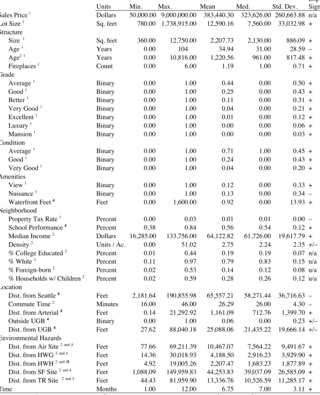
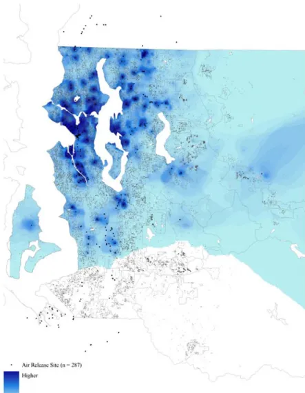
includes 29,165 transactions for single-family homes that took place during 2004 — this represents essentially all such arms-length transactions from that year. The sales data, which is mapped in Figure 3 against the backdrop of the region’s urban growth area, was stripped of all non-arms-length transactions, like those with some type of deed other than a warrantee deed, and “bad” records, with missing information or some other problem. The transactions were then loaded into a geographic information system (GIS) wherein they were linked to parcel data, also from the King County Assessor. Once this was done, the data was matched with other relevant data from the 2000 Census of Population and Housing, the Environmental Protection Agency (EPA), and various regional sources — including school district boundaries and King County’s portion of the Puget Sound’s urban growth area — to create neighborhood level and distance-based metrics. Table 1 lists the source of, and descriptive statistics for, all variables involved in the analysis.
In 2004, King County was home to over 1.75 million people, or nearly a third of Washington State’s population, living in more than 50 different jurisdictions. Within the region, there are many submarkets that can easily be distinguished on the basis of income, proximity to amenities, access to employment centers, and other factors. Nonetheless, there is considerable crossover between these submarkets because the region as a whole is exceptionally well integrated and faces little of the kind of urban decay, social turmoil, or other strife that bifurcates many other housing markets. This is not to say that income polarization and its attendant residential sorting do not exist, just not at the same extremes as they do in many other American metropolitan areas. Instead, the Puget Sound’s housing market tends to be sorted more by personal preference. For example, some residents prefer the high-density of Seattle and others
4 This information is publicly available but, for this research, it was obtained from Metroscan, a proprietary database that collects assessor’s data from King County and elsewhere.
€
prefer the low-density of the eastern suburbs and other outlying areas.5 Moreover, the Puget
Sound region in general, and Seattle — the so-called “Emerald City” — in particular, are famous for being among the nicest places to live and own housing in the United States. Views of the Cascade and Olympic mountain ranges are typical and so are views of the sound, Lake Union, Lake Washington, the Ship Canal, and many other smaller water bodies. With its large and dynamic housing market and its many opportunities to consume environmental quality, King County is an ideal setting for evaluating the demand for that commodity.
As shown in each of the first stage estimating equations — that is, in equations (1), (2) and (4) — the units of analysis are single-family homes, and the dependent variable is the natural log of sales price. By convention, these equations indicate that the price of housing depends on a vector of housing attributes, z, that describes the home itself, its neighborhood, and its location vis-à-vis amenities and disamenities. In terms of model construction, the exact set of variables that fill out this vector depends, crucially, on the geographic scope of the analysis because different things matter within different spatial frames of reference. That is, constructing a model for a specific housing submarket is a different exercise than constructing a model for all of the regional market, which is what is of interest here. With this in mind, the specification evolved throughout the course of model development and extensive sensitivity testing, along with much local knowledge, went into the end result. Throughout this work, great care was taken to ensure that the final specification was not sensitive to the inclusion or exclusion of new variables and that a high level of explanatory power was achieved.
The process of model construction led to the following nine categories of explanatory variables, some of which are captured by a lone variable: (1) lot size, measured as the square footage of the of the home’s site; (2) structure, measured as the square footage of the home, its age in quadratic form, and its number of fireplaces; (3) grade, a qualitative evaluation made by the assessor that rates the home as being of “below average,” “average,” “good,” “better,” “very good,” “excellent,” “luxury,” or “mansion” quality; (4) condition, another qualitative evaluation made by the assessor that rates the home as being in “below average,” “average,” “good,” or “very good” shape; (5) amenities, measured as whether or not the home has a view of any kind, whether or not it is subject to some sort of a nuisance, and the number of linear feet of waterfront its site has, if any; (6) neighborhood, measured as the property tax rate, calculated as the ratio of the property tax bill to the assessed value, school performance, calculated as the average percentage of students achieving success in several state aptitude tests,6 plus, defined at the
5 Charles Tiebout chose to live in Seattle itself, in a neighborhood adjacent to the University of Washington. 6 The aptitude tests are for mathematics, reading, science, and writing.
€
€
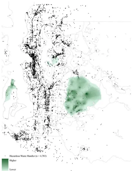
census tract level, median household income and density, calculated as housing units per acre; (7) location, measured as distance from downtown Seattle, the average commute time to work in the census tract, distance from the nearest arterial, whether or not the home is located outside of the Puget Sound’s urban growth area, and distance from the nearest point on the growth area’s boundary; (8) environmental hazards, measured as the distance from the nearest air release site, hazardous waste generator, hazardous waste handler, superfund site; and toxic release site; and (9) time, measured as the number of the month in which the home was sold. Together, these 32 variables plus an intercept form the vector z that explains the sales price of housing in King County’s portion of the Puget Sound region. The expected sign of each variable in the first stage hedonic price function is listed in the rightmost column of Table 1.
Figure 4 displays surface trends interpolated from the natural log of the sales prices of the 29,165 homes shown as points in the background of the image.7 The map reveals, on the one
hand, a richly variegated regional housing market with clearly delineated, though mostly amorphous, submarkets and, on the other hand, a high degree of spatial correlation in prices within submarkets and across the transition zones dividing them. The overall picture is one that calls upfront for an explicitly spatial modeling framework, so equations (3) and (4) already seem preferable to equation (1). The remaining issue — the fine point of the entire matter — is to determine whether or not the various housing attribute price schedules that are embedded in the Puget Sound’s single-family housing market exhibit similar patterns. If so, the information needed to expose the demand for those attributes is there too, hidden right in plain sight.
Last, before moving on to the estimates, it is necessary to provide some further detail about the five EPA designated environmental hazards that are the object of this analysis. These are: (1) air release sites, which are fixed sources of air pollution that are contained in the Aerometric Information Retrieval System; (2) hazardous waste generators, which are waste-producing facilities that are contained in the Resource Conservation and Recovery Information System; (3) hazardous waste handlers, which are handling facilities (including all waste-producing facilities) that are contained in the Resource Conservation and Recovery Information System; (4) superfund sites, which are contaminated sites prioritized for cleanup that are contained in the Comprehensive Environmental Response, Compensation, and Liability Information System; and (5) toxic release sites, which are manufactures of toxic chemicals dangerous enough to pose severe environmental and, in certain cases, public health threats, that
7 The surface trends were generated via an inverse distance weighting scheme, which is the simplest method of interpolating a surface from point data — it estimates values between observations i and j as a weighted average, where the weight given to each observation is determined by a standard distance decay function: f(dij)= 1 /dij
2
(Longley et al. 2001).
€
are contained in the Toxics Release Inventory.8 All such sites located in King County or within
five miles of its borders as of 2002, two years prior to the housing sales, are shown in Figure 3. As the pattern in the figure suggests, these environmental hazards range from everyday-type land uses, like drycleaners and gas stations, to highly stigmatized sites hosting heavy industrial activities. Accordingly, as shown in Table 1, the median home in the data set is located about: (1) 7,600 feet from an air release site; (2) 2,900 feet from a hazardous waste generator; (3) 1,700 from a hazardous waste handler; (4) 39,000 feet from a superfund site;9 and (5) 10,500 feet from a
toxic release site. However, while most homes are located far away from these sites, others are located as close as 80 feet, 15 feet, 5 feet, 1,100 feet, and 45 feet, respectively. As the figure illustrates, nearly every environmental hazard involved in this analysis is woven right into the fabric of the Puget Sound’s single-family housing market, which makes that market an ideal venue for evaluating their impacts.
3.2 First Stage Hedonic Price Function — OLS and S2SLS Estimates
The purpose of this step is to present the “global” model that was developed for the entire regional housing market and to highlight the importance of addressing the kind of localized differences in the structure of supply and/or demand that give rise to spatial non-stationarity. The main substance of the analysis lies in the GWR estimates of the first stage hedonic price function and subsequent 2SLS estimates of the second stage demand functions, so the discussion here is kept brief. But, an overview of the two global variants of the empirical model is a necessary precursor to what follows, because it establishes the econometric specification and demonstrates the high level of spatial interaction among market participants.
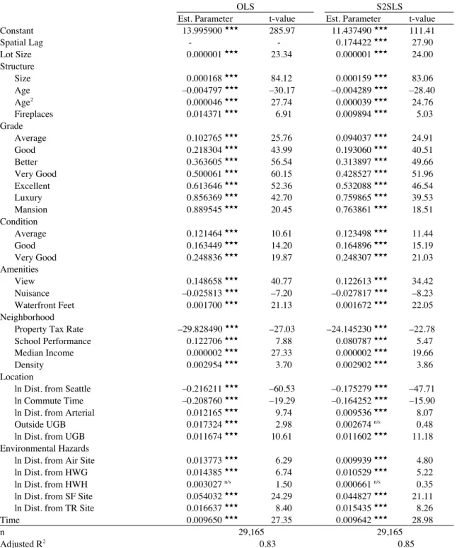
The left-hand panel of Table 2 lists OLS estimates corresponding to equation (1). Every explanatory variable carries its expected sign (if it was anticipated in advance) and all except one, distance from the nearest hazardous waste handler, is statistically significant at well over a 99% level of confidence. Overall, the vector z influences the sales price of housing in the Puget Sound region according to the expectations provided in Table 1. Furthermore, the adjusted R2 is 0.83,
indicating that the equation does an excellent job of explaining the cross-sectional variation in the sales price of single-family housing. Next, the right-hand panel of Table 2 lists the S2SLS
8 For an overview of each and access to the same data used here, see: http://www.epa.gov/enviro/html/airs/index.html for air release sites; http://www.epa.gov/epaoswer/hazwaste/data/index.htm for hazardous waste generators and hazardous waste handlers; http://www.epa.gov/enviro/html/cerclis/index.html for superfund sites; and
http://www.epa.gov/enviro/html/tris/index.html for toxic release sites.
9 Note that there are only five superfund sites in King County, so the sample is small compared to the other facilities. This poses no serious problems, but, because the region as a whole is involved in the analysis, it does make superfund sites more prone to localized idiosyncrasies — that is, if there is some kind unobserved of market anomaly nearby a superfund site, it could have an influence on the hedonic price analysis.
estimates, corresponding to equation (3), wherein the spatial lag of the dependent variable is the average price paid in the four nearest transactions.10 As expected, the autoregressive term is
positive and highly significant, which shows that the sales prices of proximate homes are strongly correlated with one another, and its inclusion in the equation raises the adjusted R2 slightly, to
0.85. The original 32 explanatory variables all have the same signs as before and, except for the variable indicating whether or not the home is located outside of the Puget Sound’s urban growth area, they all remain statistically significant at a 99% or greater confidence level. Together, the two sets of estimates contained in Table 2 represent the foundation that the remainder of the analysis rests upon.
3.3. First Stage Hedonic Price Function — GWR Estimates
As explained, GWR involves calibrating a separate regression centered on the location of every single observation in the dataset and, at the location of each regression, information from other locations is discounted with distance from it, so that closer observations have a greater influence on the model’s solution. The technique, which is computationally complex and requires specially developed software (Fotheringham et al. 2003), produces output consisting of a voluminous total of n ⋅k parameters — so, in this case, 962,445 (or 29,165 ⋅ 33) location-specific estimates.
Before discussing the findings, a remaining aspect of the GWR procedure, the determination of the appropriate spatial bandwidth, needs some explanation because it affects the estimation results. There are two options: (1) a fixed spatial bandwidth, which uses all observations, no matter how few or how many, located within a constant radius of the regression point, so the sample size varies by location; and (2) an adaptive spatial bandwidth, which uses a constant number of observations, no matter how close or how far away they are from the regression point, so the sample size does not vary by location. Compounding this choice, the GWR software can be used to find a statistically “optimal” bandwidth or it will let the user supply a predetermined bandwidth. Various combinations of these alternatives were explored for the purposes of this research and, in the end, an adaptive spatial bandwidth encompassing 21,874 nearest neighbors — a constant 75% of the dataset — was used to generate the estimates. Any further details on the estimation process are available upon request from the corresponding author.
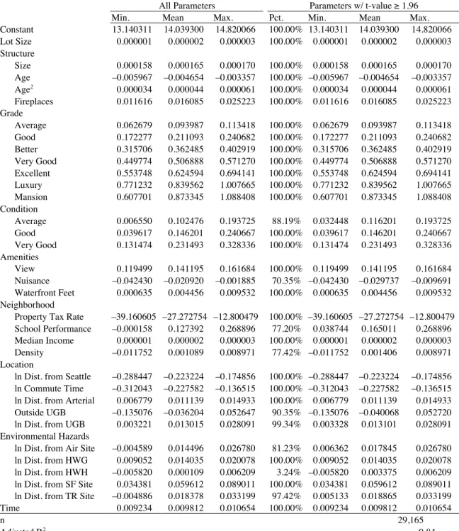
Getting into to the findings, Table 3 lists GWR estimates corresponding to equation (4). The left-hand panel of the table gives the minimum, mean, and maximum value of all parameters
10 All spatially lagged variables were generated in GeoDa (see Anselin et al. 2006), and then imported into EViews, where the OLS, STSLS, and 2SLS equations described in this paper were estimated.
€
€
€
€ €
estimated in the procedure and the right-hand panel gives the same numbers but only for those parameters having t-values ≥1.96. As the column in the right-hand panel listing the percentages demonstrates, for almost all of the variables, every single location-specific parameter is significant at a 95% or greater level of confidence. For most of those that do not meet the 100% mark, the rate of statistical significance is still very high. The one exception, as in the global estimates, is distance from the nearest hazardous waste handler, which is only statistically significant 3.24% of the time. Overall, the sign pattern in Table 3 is the same as the sign patterns in Table 2. The only variable that deviates from this is neighborhood density, which breaks in both directions, from a minimum of –0.012 to a maximum of 0.009. This indicates that, other things being equal, in some locations, density raises the price of housing and, in other locations, it lowers the price of housing. Figure 5, which shows surface trends interpolated from the density parameter estimates (γˆik), illustrates that the pattern is systematic. Specifically, as telegraphed in the discussion above, density has a positive influence in the western half of King County and a negative influence in the eastern half. Anecdotally, it is something of a cliché among urban planners in the Puget Sound that the two things residents dislike most are density and sprawl, and, so, this is one of the ways in which the housing market there is segmented. The figure reflects the impact of households with preferences for density bidding up the price of housing for that attribute in Seattle and its immediate vicinity and, conversely, the impact households with preferences against density bidding down the price of housing for that attribute in the region’s eastern suburbs.11 The adjusted R2 of the GWR model is 0.84 and the Akaike Information
Criterion (AIC) statistic is –17,553.67, an improvement over the –15,033.12 of the OLS variant of the model.
Most important, some of the GWR parameter estimates exhibit wide ranges in value, suggesting that spatially distinct price schedules for those attributes may indeed be embedded in the regional housing market (Can 1990, 1992). Because the dependent variable is in natural log form, the marginal implicit prices from the hedonic price function are πˆik= γˆik⋅pi or, where the explanatory variable is also in natural log form, πˆik= γˆik⋅pi/ zi. The product of the relevant term and zi gives the value of the estimated total implicit expenditure, ηˆik. In cases where the location-specific parameter is not statistically significant, the marginal implicit price was taken to be zero because insignificance means, after all, that the variable had no influence on sales price. The minimum, mean, and maximum values (accounting for zeros) of the estimated marginal
11 To the authors, who know the Puget Sound region well, this result serves as a conformation that the GWR parameter estimates reflect true patterns of spatial non-stationarity.
€
€
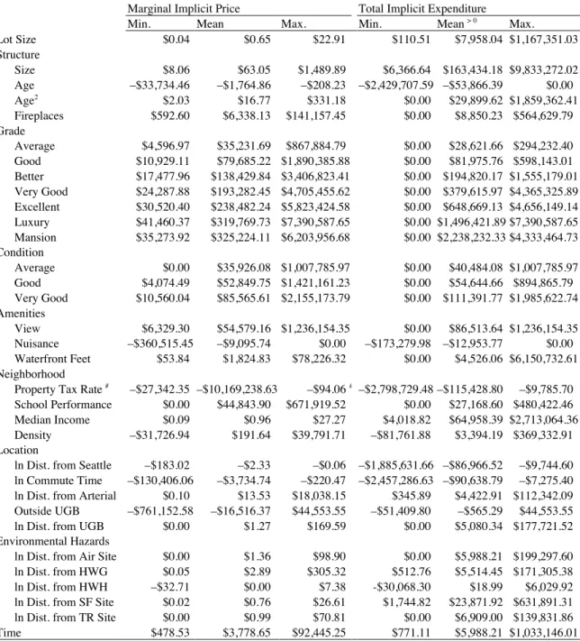
implicit price of, and total implicit expenditure on, each attribute are listed in the left-hand and right-hand panels of Table 4, respectively.
Because sales price and the distances from the five environmental hazards are all expressed in natural log form, the distance parameters are elasticities. On average, these elasticities reveal that preferences for this form of environmental quality are ordered as follows: superfund sites (0.06) > toxic release sites (0.02) > air release sites (0.017) > hazardous waste generators (0.01) > hazardous waste handlers (0.003). And, as the marginal implicit prices shown in the left-hand panel of Table 4 reveal, the average transaction contributed: (1) $1.36 for an additional foot of distance from the nearest air release site; (2) $2.89 for an additional foot of distance from the nearest hazardous waste generator; (3) $0.00 for an additional foot of distance from the nearest hazardous waste handler; (4) $0.76 for an additional foot of distance from the nearest superfund site; and (5) $0.99 for an additional foot of distance from the nearest toxic release site. These are the mean values of πˆik, the estimate of marginal implicit price required for the second stage demand functions. Note, however, that these estimates are average prices per foot of distance across all distance consumed and that, because of diminishing marginal utility, the first foot of distance from an environmental hazard is far more expensive than, say, the 40,000th foot. A clearer picture emerges, then, from the total implicit expenditures,
ηˆik, which are listed in the right-hand panel of Table 4. The table shows that the average home, which sold for $383,440, involved a total implicit expenditure of: (1) $5,988.21 on distance from the nearest air release site; (2) $5,514.45 on distance from the nearest hazardous waste generator; (3) $18.99 on distance from the nearest hazardous waste handler; (4) $23.871.92 on distance from the nearest superfund site; and (5) $6,909.00 on distance from the nearest toxic release site.
Surface trends interpolated from the 29,165 location-specific marginal implicit prices of distance from air release sites, hazardous waste generators, hazardous waste handlers, superfund sites, and toxic release sites are shown in Figures 6 – 10. The maps are revealing because they show exactly where and how the five environmental hazards have impacted King County’s single-family housing market. In some parts of the region, which have been left white, air release sites, hazardous waste handlers, and toxic release sites have had no effect but, overall, the influence of the facilities is wide ranging. A striking feature of the maps is that the marginal implicit prices of distance from the hazards are spatially incongruent — the patterns of impact vary across the five types of facilities, and even within each type. This latter finding is consistent with a recent analysis of superfund sites by Kiel and Williams (2007), who found that that the impact on housing markets varies substantially from site-to-site. Note, too, that the patterns of impact shown in Figures 6 – 10 illustrate why homes located far from the environmental hazards
€ € € € € € € € € € €
do not necessarily end up with large total implicit expenditures on distance. In particular, even though the amount of distance consumed is large for more distant homes, the marginal implicit price of distance is very small, so the product of the two (ηˆik) does not have to be big. Had the maps been created using the stationary OLS or S2SLS parameter estimates, they would illustrate a situation wherein the total implicit expenditure on distance would always rise with distance, even if marginally. Instead, because of the non-stationary parameters, homes located close to environmental hazards can (and commonly do) end up having greater total implicit expenditures than those located further away.
Recall now that it is possible to estimate second stage demand functions for environmental quality if spatially segmented submarkets having separate hedonic price schedules for the identical attributes are available. A lone hedonic price function cannot be used to do this because it is a composite of both supply and demand and, so, does not contain the information needed to identify the second stage function. Table 4 reveals that the marginal implicit price of, and total implicit expenditure on, many of the housing attributes included in the first stage function have considerable range, but this, while promising, is not in-and-of-itself evidence of spatially segmented submarkets. What is needed to confirm the presence of segmentation, is a test of whether the variances of the total implicit expenditures described in the right-hand panel of the table are owed to variation in the attributes or, instead, to variation in the marginal implicit prices. In other words, the question is: Does the variance of each ηˆik across the 29,165 transactions come from variation in zk, the quantity consumed, or from variation in πˆik, the marginal implicit price? Evidence that the latter is responsible for the variance of ηˆik is needed to establish that the kind of spatially segmented markets that give rise to non-stationarity housing attribute price schedules are present. If such submarkets exist, then so, too, does the information needed to identify the second stage demand functions for environmental quality.
Ali et al. (2007) have developed just the test needed to ascertain this. Following their approach, the variance of the total implicit expenditures was decomposed via the following:
var(ηˆ ik) = (∂ηˆ ik/∂zk)2 ⋅ var(z
k) + (∂ηˆ ik/∂πˆik)2 ⋅ var(πˆik) (5)
+ 2 ⋅ cov(πˆik,zk) ⋅(∂ηˆ ik/∂zk) ⋅ (∂ηˆ ik/∂πˆik).
In this formula, the partial derivative in the first term is the mean of πˆik2 ; the partial derivative in
the second term is the mean of zk2; and the partial derivatives in the third term are the means of πˆik and zk. The terms themselves give the share of the variance in ηˆ ik, total implicit
€
€ € €
€ €
€ € €
expenditures, that is attributable to: (1) spatial variation in zk, the attributes; (2) spatial variation in πˆik, the marginal implicit prices; and (3) the covariance of πˆik and zk.12
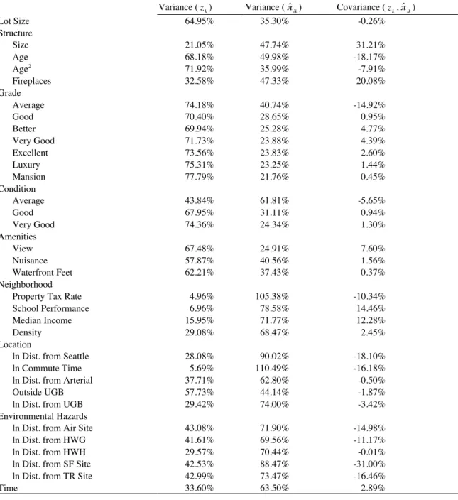
The results of Ali et al.’s (2007) spatial decomposition test, which are presented in Table 5, are compelling. Just as earlier findings (Michaels and Smith 1990) seem to indicate, certain total implicit expenditures vary significantly due to spatial non-stationarity in marginal implicit prices but others do not. For many of the housing attributes that are characteristics of the home itself, much, if not most, of the variance in ηˆ ik is owed to spatial variation in zk. For example, there is little evidence of a spatially segmented implicit market for lot size — about two thirds of the total implicit expenditure is owed to the quantity consumed — so the hedonic price schedule for that attribute is relatively constant across King County. Other things being equal, an additional square foot of lot costs more-or-less the same anywhere within the regional housing market. Further down the list of explanatory variables, though, the opposite is true. For attributes that are spatial in nature, and particularly for distance from the five environmental hazards, there is overwhelming evidence that the variance in ηˆ ik is owed to spatial variation in πˆik, not zk. Specifically, spatial variation in marginal implicit prices accounts for the majority of the variance in total implicit expenditure on distance: (1) 72% for air release sites; (2) 70% for hazardous waste generators; (3) 70% for hazardous waste handlers; (4) 88% for superfund sites; and (5) 73% for toxic release sites. In short, the total amount that households spent on avoiding these facilities depends largely on how distance from them was priced at the location of the home they purchased. This segmentation may be due to asymmetrical information, barriers to market entry, or any other factor causing idiosyncratic differences in the structure of supply and/or demand. Whatever the reason, it means that the kind of spatially distinct submarkets needed to identify second stage demand functions for these attributes is there, hanging in the aether of the regional housing market.
3.4 Second Stage Demand Functions — 2SLS Estimates
Like other hedonic price analyses involving second stage estimation (see, for example, Brasington and Hite 2005) this research relies on spatial variation in housing attribute price schedules to address the identification problem. The main difference is that, instead of using different regions as distinct housing market segments, this analysis leverages spatial non-stationarity in housing attribute prices within a single region to identify the second stage demand
12 Ali et al.’s (2007) test deals with a somewhat simpler situation wherein the term that is decomposed is the product of the GWR parameters and the explanatory variables. Since marginal implicit prices are the object of interest here, the actual values of the GWR-estimated housing attribute price schedules first had to be backed out of the log-transformed equations.
€ € € € € € € €
functions. With the marginal implicit price estimates, πˆik, from the first stage hedonic price function in hand, the remaining step of the analysis is to estimate a series of second stage demand functions corresponding to equation (3).
As already explained, the dependent variable of these functions is quantity — expressed as q˜ik , the natural log of distance from each environmental hazard — and the explanatory variables are the marginal implicit price of distance, the marginal implicit prices of distances from the other hazards, which may act as compliments or substitutes, and a standard set of demand shifters. Because πˆik is endogenous to q˜ik , the demand functions must be estimated via two stage least squares (2SLS) or some other instrumental variables procedure. The instruments used to do this are all of the exogenous variables, plus spatial lags of those same variables, or, in matrix form, X and Wij⋅X.13 The 2SLS estimation results for the implicit markets for distance
from air release sites, hazardous waste generators, hazardous waste handlers,14 superfund sites,
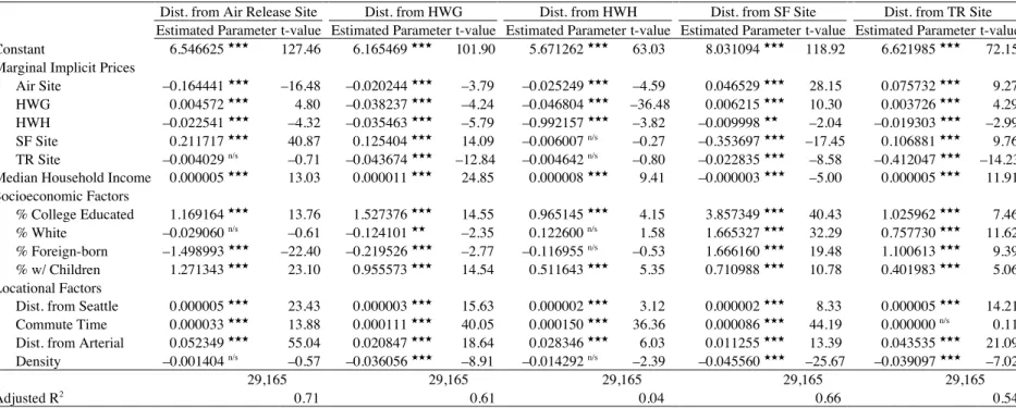
and toxic release sites are listed from left to right, respectively, in Table 6. Each of the equations except for the one for hazardous waste handlers registers a respectable adjusted R2 and almost all
of the explanatory variables are statistically significant and appropriately signed. The next paragraphs summarize the own-price, income, and cross-price relationships and the influence of the set of demand shifters in turn.
The equations are all in semi-log form so own-price elasticities can easily calculated, by taking the product of the estimated parameter and the mean of the estimated marginal implicit price: δˆ ⋅πˆik. As expected, all of the price elasticities of demand that come out of this calculation are negative, or, in one instance, essentially zero: (1) –0.22 for air release sites; (2) –0.11 for hazardous waste generators; (3) 0.00 for hazardous waste handlers; (4) –0.27 for superfund sites; and (5) –0.41 for toxic release sites. These results are remarkably consistent with work done by Brasington and Hite (2005), who found a price elasticity of demand of –0.12 for an almost identical measure of environmental quality.15 In general, it is reasonable to expect high profile
environmental hazards to not only generate large implicit price responses in the first stage hedonic price function but, also, to generate large distance responses in the second stage demand functions. And, for this reason, it is interesting that all of the price elasticities of demand are less than one, indicating that demand is inelastic. This finding suggests that household responses are relatively stronger in the first stage hedonic price function than in the second stage demand
13 Just as before, W
ij is an n ×n spatial weights matrix and the spatial lags give the average of values from the four
nearest neighbors.
14 The implicit price of distance from hazardous waste handlers was zero for 28,220, or about 97%, of the observations. 15 Distance from the nearest Ohio Environmental Protection Agency designated environmental hazard
functions — households apparently do not mind proximity to environmental hazards as long as they are compensated for it.
Beyond this, the relative ordering of the price elasticities of demand is reasonable: Toxic release sites > superfund sites > air release sites > hazardous waste generators > hazardous waste handlers. This lines up well with the levels of risk actually associated with the five environmental hazards. In particular, the largest own-price elasticity is for toxic release sites, which are facilities registered in the Toxics Release Inventory, a publicly available database of firms that emit toxic chemicals into the environment.16 Given the severe stigma attached to many of these facilities, it
is not surprising that they have the highest of the five price elasticities of demand. The result for superfund sites may initially seem counterintuitive given their high profile, but it is actually not, considering that operations at these facilities have ceased and, so, no further contamination is likely to happen. Indeed, research on a superfund site located in nearby Tacoma, Washington by McMillen and Thorsnes (2003) found that superfund designation eventually leads housing values to rebound from initial losses in anticipation of cleanup. The price elasticity of demand for distance from air release sites is comparable to the price elasticity of demand for distance from superfund sites, and this may be attributable to the high visibility that air release sites can have. Public knowledge is at the core of how environmental hazards influence the housing market, and the evidence here suggests that emissions from air release sites send comparatively strong signals to market participants. The remaining two hazards, hazardous waste generators and hazardous waste handlers, tend to be everyday-type land uses and, for this reason, households exhibit less aversion to living in close proximity to them and their own-price elasticities are correspondingly low.
Income elasticities of demand for each of the five hazards are calculated the same way as before, by taking the product of the estimated parameter and the mean of median household income. Note, however, that interpretations have to be tempered by the fact that the measure of income is calculated at the census tract level because household level data corresponding to the single-family housing sales was not available. That said, as expected, all of the income elasticities of demand that come out of this calculation except one are positive: (1) 0.32 for air release sites; (2) 0.71 for hazardous waste generators; (3) 0.51 for hazardous waste handlers; (4) –0.19 for superfund sites; and (5) 0.32 for toxic release sites. Overall, these values imply that environmental quality is a normal good so, other things being equal, households spend more on it as their incomes rise. As to how readily: Hazardous waste generators > hazardous waste handlers
16 The inventory was created in response to the 1984 Bhopal, India accident wherein a Union Carbide plant accidentally released a large volume of methyl isocyanate gas. By some estimates, more than a million people were exposed to the gas, and more than 20,000 eventually died from their exposure to it.
> air release sites > toxic release sites. The perverse sign on the one elasticity suggests that superfund sites are not normal goods, but this may be due to some anomaly stemming from the small number of them involved in the analysis. As footnoted above, the fact that there are so few within such a large market significantly increases the chances for the estimation results to be distorted by an unobserved factor so, whatever the exact cause of the result, it is almost certainly spurious.
Next, the parameter estimates on the exogenous marginal implicit prices in each equation reveal which forms of distance are complements and which forms of distance are substitutes. To give two examples: (1) in the implicit market for distance from air release sites, distance from hazardous waste handlers is a complement and distance from hazardous waste generators and distance from superfund sites are substitutes; and (2) in the implicit market for distance from superfund sites, distance from hazardous waste handlers and distance from toxic release sites are complements and distance from air release sites and distance from hazardous waste handlers are substitutes. Note that each equation deals with a separate implicit market so there is no reason to expect symmetry among complements and substitutes — that is, theory does not dictate that one hazard is a substitute for, or complement to, another just because there is a relationship the other way around. Though detailed discussion of the cross-price relationships is beyond the scope of this paper, any subsequent welfare analysis aimed at estimating the benefits of site remediation, for example, would involve examining them more thoroughly.
Last, the two groups of demand shifters illustrate how various socioeconomic and locational factors affect the quantity of distance from environmental hazards that households consume. The initial group shows that quantity is positively influenced by: (1) education, measured as the percent of residents in the census tract that are college educated; (2) absence of racial minorities, measured the percent residents in the census tract that are white; and (3) the presence of children, measured as the percent of households in the census tract with children. The percent of residents that are foreign-born in the census tract negatively influences distance from air release sites and hazardous waste generators but positively influences distance from superfund sites and toxic release sites. Meanwhile, the second group of demand shifters shows that quantity is positively influenced by: (1) distance from downtown Seattle; (2) commute time; and (3) distance from the nearest arterial. It also shows that quantity is negatively influenced by neighborhood density, which, other things being equal, directly impacts the ability of households to live away from environmental hazards. Each of these findings is intuitive, except, perhaps, the mixed result for foreign-born residents, which merits further investigation. In addition to playing their own part in the equations, the demand shifters, by virtue of their sound performance,