Winter road maintenance resource allocation models

(1)

WINTER ROAD MAINTENANCE RESOURCE ALLOCATION MODELS

A Master’s Thesis presented to

the Faculty of the Graduate School University of Missouri

In Partial Fulﬁllment

of the Requirements for the Degree Master of Science

by

ZHONGWEI YU

Dr. Wooseung Jang, Thesis Supervisor

(2)

The undersigned, appointed by the Dean of the Graduate School, have examined the dissertation entitled:

WINTER ROAD MAINTENANCE RESOURCE ALLOCATION MODELS

presented by Zhongwei Yu,

a candidate for the degree of Master of Science and hereby certify that, in their opinion, it is worthy of acceptance.

Dr. Wooseung Jang

Dr. Mustafa Sir

(3)

ACKNOWLEDGEMENTS

It would not have been possible to write this master thesis without the help and support of the kind people around me, for whom I would like to show my gratefulness here.

I owe my deepest gratitude to my parents, Hanhe Yu and Guangping Guo, who gave me life in the ﬁrst place, encouraging and supporting me by all means.

I am heartily thankful to my advisor, Dr. Wooseung Jang, not only for guiding and supporting me, but more importantly, for giving me the opportunity to be involved in the winter road maintenance project, which inspired me to write this thesis. He was always there to meet me and discuss my ideas, help me solve research problems and review my paper chapter by chapter.

Besides, I would like to thank the rest members of my thesis committee: Dr. Mustafa Sir and Dr. Oksana Loginova, who gave me insightful comments and asked me good questions to improve my thesis.

A special thanks goes to Dr. Cheng-Hsiung Chang and Dr. Luis Occena, who rescued me from my life crisis. I could not have ﬁnished my thesis without their encouragement and constant support.

I would also like to thank my friends: Qiuming Yao, Beilei Zhang, Zhe Zhang, Yi Zhang, Gaohao Luo, Wilfred Fonseca and many other friends for their kindness, friendship and support to help me settle down in the new environment.

(4)

(5)

3. WINTER ROAD MAINTENANCE MODEL . . . 13

3.1 Relevant Components . . . 14

3.1.1 Service Area . . . 14

3.1.2 Storm Factors . . . 14

3.1.3 Service Resource. . . .15

(6)

4. SOLUTION APPROACHES . . . 22

4.1. When Feasible Solutions Exist . . . 22

4.2. When Feasible Solutions Do Not Exist . . . 23

5. CASE STUDY . . . 36

5.1. Case Background . . . 36

5.1.1. Overview . . . 36

5.1.2. Winter Road Maintenance Operations . . . 37

5.1.3. Winter Road Maintenance Network . . . 38

5.1.4. Winter Road Maintenance Resources . . . 40

5.2. Model Parameters . . . 40 5.2.1. Considered Area . . . 40 5.2.2. Storm Factors . . . 42 5.2.3. Service Resource . . . 45 5.3. Case Results . . . 46 6. CONCLUSIONS . . . 56 APPENDIX 1. APPENDIX A . . . 59 2. APPENDIX B . . . 61 3. APPENDIX C . . . 62 4. APPENDIX D . . . 63 BIBLIOGRAPHY . . . 64

(7)

LIST OF FIGURES

Figures Page

Figure 5.1 Counties in Central Missouri . . . 37

Figure 5.2 Service Regions in Central Missouri . . . 41

Figure 5.3 Reallocation (Scenario 1) . . . 52

Figure A.1 Matlab Code Part 1 . . . 59

Figure A.2 Matlab Code Part 2 . . . 60

Figure B.1 Service Regions and Depot Locations . . . 61

Figure C.1 Snowfall Averages . . . 62

(8)

LIST OF TABLES

Tables Page

Table 4.1 Reallocation Unit Cost . . . 24

Table 5.1 Three-Class Hierarchy . . . 39

Table 5.2 Service Frequency by Class . . . 41

Table 5.3 Roadway Information . . . 42

Table 5.4 Storm Impact on Service Speed . . . 43

Table 5.5 Storm Probabilities in Each Region (Scenario 1) . . . 44

Table 5.8 Original Number of Trucks . . . 45

Table 5.9 Number of Trucks (Scenario 1) . . . 46

Table 5.12 Level of Service (Scenario 2) . . . 49

Table 5.13 Level of Service (Scenario 3) . . . 49

Table 5.14 Reallocation Plan (Scenario 1) . . . 51

Table 5.17 Level of Service after Reallocation (Scenario 2) . . . 53

(9)

WINTER ROAD MAINTENANCE RESOURCE ALLOCATION MODELS

Zhongwei Yu

Dr. Wooseung Jang, Thesis Supervisor ABSTRACT

Winter snow storms could cause serious disruptions to traffic and transportation. Because resources for winter road maintenance, such as snow removal trucks, are limited, using them properly would improve the efficiency and effectiveness of the winter maintenance work. However, a fixed resource allocation plan among service regions may not work well in several situations because of different types and intensity of winter storms. Therefore, reallocation of resources among service regions is often needed. The objective of this research is to develop a resource reallocation model that minimizes the total cost of reallocation operations and provides equitable resources to service regions. Road and weather condition factors, such as road classes, weather forecasts, and service levels, are taken into account in the model.

(10)

Chapter 1

Introduction

Resource allocation operation is the process of distributing limited resources to satisfy various demands in different locations. This kind of problem is especially important when an emergency happens. When natural disasters, such as earthquakes, tsunamis and blizzards, strike certain areas, it is urgent to find the best assignment of available rescue resource so that more people can be saved. On the other hand, if the threat is partially predictable, for example, by forecasting the storm or hurricane movement, it would be more efficient and economical to reallocate the resource before the emergency happens.

In winter, snow storms could cause serious disruptions to traﬃc transportation, because it is hard to drive on slick roads which are covered by ice and snow. According to the statistics of the Federal Highway Administration, 24 percent of weather-related vehicle crashes occur on snowy, slushy, icy roads and 15 percent happen during snow-fall or sleet each year. Therefore, winter maintenance work, including spreading salts and abrasives, snow plowing, loading snow into snow removal vehicles and hauling snow to disposal sites, is of great importance to decrease traﬃc accident risk in winter. One of the most important winter maintenance resources is the snow removal truck, which is used to clear snow-clad roads. Since the quantity of snow removal trucks is

(11)

always limited due to ﬁscal constraints, deploying them properly would help improve the level of winter maintenance service.

In this thesis, we consider the situation where a certain area is under the threat of winter storms. There are several districts in this area, and each district owns a road maintenance depot which carries a certain number of snow removal trucks. Based on the characteristics of districts, such as road condition, number of trucks, snowfall intensity, etc, it is reasonable to imagine that some of the districts would have the capability to maintain a high level of service during a snow storm, while others not. Hence, reallocating the snow removal trucks in this area is eﬀective in improving the winter maintenance service quality in the whole area.

In the state of Missouri, more than 1,800 vehicles are available for snow removal work in winter on the state’s 32,000-mile highway system. The work is divided among 10 districts. The traditional method of solving these maintenance problems is highly empirical in nature. Most of the decisions on deploying snow removal trucks are typically made by district supervisors, based on the ﬁrst hand reports and personal experience. It is hard to adjust the amount of snow removal trucks in each district in a global perspective, and decisions made too late delay the dispatch of snow removal vehicles, decreasing the eﬃciency of winter road maintenance work.

Our objective of this research is to develop a resource allocation model for winter maintenance work in the considered area. In this model, reallocation operation is performed before a storm strikes, and a certain level of winter maintenance service is maintained in each district after reallocation. The goal of the model is to minimize the total reallocation operation cost under service level constraints.

(12)

Chapter 2

Literature Review

2.1

Typical Winter Road Maintenance Models

Winter road maintenance operations include spreading of salts and abrasives, snow plowing, loading snow into snow removal vehicles and hauling snow to disposal sites. Due to the complexity of the operations, various models have been introduced to the planning and management of winter road maintenance work. Although these models emphasize different aspects of winter road maintenance operations, their objectives are typically the same, i.e. minimizing the sum of the operational costs. Most of the existing models can be classified into three major fields: vehicle routing, depot location and fleet sizing.

2.1.1

Vehicle Routing and Scheduling

Within these models, vehicle routing problems received the most attention because these operations are common to snow ﬁghting in all urban and rural regions. These problems are practical examples of the Chinese Postman Problem and related arc routing problems, and are similar to other arc routing problems such as garbage collection and street sweeping.

(13)

snow disposal routing. Spread routing problems concern the operations of spreading chemicals and abrasives, while plow routing problems focus on the removal of snow from the road, and snow disposal routing problems deal with loading snow and hauling snow to the disposal sites. The first two problems both consist of determining a set of routes, each performed by a snow-fighting vehicle that starts and ends at its own depot, so that all districts are served, every operational constraint is satisfied, and more importantly the global cost is minimized. However, the snow disposal routing problem is more complicated, which determines the best set of itineraries for the trucks filled with snow that travel from the assigned snow blower site, to disposal sites, and back to the snow blower site such that the total cost is minimized. Both spread routing and plow routing problems can be generally formulated as arc routing problems, the snow disposal routing problem is a more difficult shortest path problem. Marks and Sticker (1971) modeled the plow routing problem as a multiple vehi-cle undirected Chinese Postman Problem, and proposed two approaches – a route first-cluster second approach and a cluster first-route second approach – to solve it. Eiselt et al. (1995) presented a review on arc routing problems, and gave the algo-rithmic results for Chinese Postman Problems under different conditions. A typical scheduling problem is presented by Lu, et al. (2009), who described a routing prob-lem of winter road maintenance, considering the operating costs, quality of service and weather condition factors, and then established a linear model to find out the optimized schedule for assigning routs, service type and corresponding start time.

(14)

2.1.2

Depot Location and Sector Design

Depot location and sector design involve ”partitioning the geographic region into sec-tors for efficient operations, locating the necessary facilities, and assigning the secsec-tors obtained from the partitioning to various facilities” (Pierrier, et al. 2006). Similarly to the vehicle routing problems, sector design and depot location problems can be classified into two kinds of problems: sector design for spreading and plowing and sector design for snow disposal. The sector design problem for spreading and plowing consists of partitioning a spreading or plowing route network into non-overlapping subnetworks, and assigning vehicle depots to these sectors, such that the transport costs and vehicle depot costs are minimized. It is similar to the arc partitioning problem in the context of postal delivery and districting problems for arc routing applications. On the other hand, given a road network and a set of planned dis-posal sites, the sector design problem for snow disdis-posal consists of determining a set of non-overlapping subnetworks, and assigning each sector to a single snow disposal site in order to minimize the relevant variable and fixed costs. Solution approaches for both problems are similar. Korhonen et al. (1992) developed a decision support system allowing managers to select vehicle depots and their corresponding sectors such that variable transport cost and fixed vehicle depot costs are minimized. The model was solved by a construction heuristic that opens depots sequentially until no further savings are realized. Perrier et al. (2008) provided a mathematical model of sector design and assignment of sectors to disposal sites, and proposed two construc-tive approaches – the assign first, partition second method and the partition first, assign second method – to solve it. The result of Perrier’s experimentation showed

(15)

that the assign-partition heuristic could result in substantial savings compared to the partition-assign approach.

2.1.3

Fleet Sizing and Replacement

Fleet sizing problems consist of determining the number of winter maintenance ve-hicles from depots such that the total operational and depot depreciation costs are minimized, while a specified level of service for each road class is satisfied. Accord-ing to the types of winter maintenance operations, the fleet sizAccord-ing problems can be divided into two classes: fleet sizing for plowing and fleet sizing for hauling snow to disposal sites. The difference between the two problems is that fleet sizing for plowing balances the total costs and the length of time to plow each class road, while fleet sizing for snow disposal balances the total costs and the length of time for the snow loading and hauling operations.

Fleet replacement or fleet design considers the cost of purchasing, operating, main-taining and replacing vehicles in a fleet. These kind of problems determine a replace-ment schedule (i.e. how many replacereplace-ment groups the fleet should have, how large each replacement group should be, the age at which each group is replaced and the relative distribution of the groups overtime), so that the total costs of operating, maintenance and net replacement are minimized. Jones (1993) considered a general fleet design problem in a simplified economic environment, and developed the first formal model that determines optimal steady-state fleet design. The research showed that all replacement groups must be equally sized in the optimal steady-state fleet design.

(16)

2.1.4

Integrated Winter Road Maintenance Model

Although the winter maintenance models above are most often solved separately, there are still strong interactions between them. For example, in the vehicle routing problem, each route starts from a depot and ends at a depot, and a set of routes complete the service in a sector. Therefore, vehicle routing problems always correlate with depot location or sector design problems. Hayman and Howard (1972) generated a compound model of sector design, depot location and ﬂeet sizing. Lotan, et al. (1996) discussed a problem combining the depot location and routing problems for spreading. Zhang, et al (2006) developed an integrated system which considers the optimization models and solution algorithms for the routing of snow removal trucks and the location of road maintenance depot in Boone County, MO, and proposed a route ﬁrst-cluster second approach based on Marks and Sticker’s (1971) method.

2.2

Resource Allocation Problems

Resources are meant to be limited in every aspect of life, however, there are always various demands among different functional parts of a system that need to be satis-fied. Therefore, how to allocate the limited amount of resources so as to achieve a high performance of the system would be a problem that every organization encounters. In winter road maintenance problems, snow-fighting vehicles such as snow plowing trucks might be the most important resource. Recall the typical winter maintenance models; almost every model considers the number of snow-fighting vehicles available as the primary factor. Then the winter road maintenance resource allocation prob-lem becomes determining a plan that allocates the limited number of snow-fighting

(17)

vehicles in order to achieve a high level of service. Eﬃciency and eﬀectiveness are the two parameters that measure the primary aspects of winter maintenance work.

2.2.1

Eﬃciency-oriented model

Efficiency generally concerns the cost associated with doing business. In other words, the objective of an efficiency-oriented resource allocation model is minimizing the total operational cost, while several effective constraints may need to be satisfied. One of the most solved efficiency-oriented problems is the Hitchcock transportation problem. A typical transportation problem aims to find the best strategy of fulfilling the demands of a set of destinations using the supplies of a set of sources. While trying to find the best way, a variable cost of shipping the commodity from one source to a destination, as well as the capacity of supply in each source and the minimum demand in each destination should be taken into consideration. The objective of a typical transportation problem is to minimize the sum of all incurred transportation costs. Due to its special mathematical structure, several efficient solution approaches based on the simplex method have been developed. These methods differ in how to calculate the necessary simplex-method information.

In 1951, the primal simplex transportation method was proposed by Danzig, who adapted the simplex method to the transportation problem. Charnes and Cooper (1954) developed the stepping- stone method, in which unused cells in transportation tableaus were referred to as ”water” and used cells as ”stones” – from the analogy of walking on a path of stones half-submerged in water. The stepping-stone method is much easier to comprehend, because most of the solution procedures are conducted on transportation tables. However, it is not applicable to all types of linear programming

(18)

problems. Besides, it is not even suitable for transportation problems with a large number of origins or destinations. Arsham and Kahn (1989) provided a simplex-type tableau-dual algorithm which is an alternative to the stepping-stone method for general transportation problems. This algorithm only has one operation – Gauss Jordan pivoting in transportation tableau, and all operations can be performed in a single working tableau. In addition to these simplex-type methods, some heuristics were also introduced: Vignaux and Michalewicz (1991) used a genetic algorithm to solve the linear transportation problem; Adlakha and Kowalski (2003) presented a simple heuristic algorithm to solve the ﬁxed-charge transportation problem.

2.2.2

Eﬀectiveness-oriented model

Effectiveness generally concerns the resulting outcome, which means the objective of an effectiveness-oriented model is maximizing the outcome after allocation, while several efficiency constraints may be included. There are quite a few resource allo-cation models with the objective functions that minimize the total cost of alloallo-cation operations, however, when the loss incurred by inadequate resources is invaluable, compared with the cost of allocation operations, the objective of this kind of resource allocation models changes to the optimization of the outcome: minimization of the loss caused by the unavailable resources, in many cases.

For instance, when natural disasters like earthquakes happen, it is urgent to send rescue teams and equipments to the aﬀected areas in the ﬁrst few days, otherwise more people would be killed. The maximum time of survival lies between four and seven days, and the probability of survival decreases to zero in one day if the trapped person is injured. Since the quantity and quality of the rescue resources are limited,

(19)

the emergency manager has to find the best assignment of available resources, so that more people can be saved in the shortest time. Fiedrich et al. (2000) introduced a dynamic resource allocation model for the search-and-rescue operations after earth-quakes, of which the goal is to minimize the total number of fatalities. In his model, three different rescue tasks – rescuing people out of the collapsed buildings, stabiliz-ing work to prevent second disasters and rehabilitation of transportation lifelines to improve the accessibility of important areas, are taken into consideration. Thus, res-cue resources are classified into corresponding categories, and the maximum volume of each resource is used as the restriction that should be fulfilled in the model. Two heuristic methods – Simulated Annealing and Tabu Search are introduced to solve this resource allocation problem.

As mentioned above, time seems to be the most important factor that affects the total number of fatalities. Therefore, instead of the total number of fatalities, time could also be used as the measure of allocation performance. In Gong and Batta’s (2007) ambulance allocation and reallocation model, the objective becomes minimization of makespan, which is the maximal finish time of the rescue operation in each cluster, or minimization of the total flow time, which means the summation of the finish time of rescue operations in all clusters. Gong and Batta first formulated the deterministic model that concerned the allocation of the correct number of ambulances at the beginning of the rescue operations. Moreover, since the situation in each cluster changes during the rescue period, the former ambulance plan may not be optimal in the new period. As a result, a reallocation model with the objective of minimizing the makespan over discrete time period was proposed. Both the ambulance allocation

(20)

and reallocation problems can be solved by an iterative procedure presented by Gong and Batta.

2.2.3

Fair Allocation

Efficiency and effectiveness are common measures of a resource allocation system performance, nevertheless, only minimizing the total cost or maximizing aggregate outcome may be extremely unfair in systems which serve many different demands. One of the widely used fair allocation models is the so-called Min-Max model, which tries to find the best allocation of limited resources to a given set of demand sites, so that the maximum of the profit or loss differences between the demand sites is minimized.

Much research has been conducted on the Min-Max fair allocation model. Zeitlin (1981) first considered the Min-Max resource allocation problem with discrete re-sources. Katoh et al. (1985) presented a more general model, whose constraints include the fixed size of discrete commodity and lower and upper bounds on the amount of the commodity to be allocated to each demand site. Tang (1988) for-mulated several manufacturing problems into a max-min resource allocation model, and developed a procedure that finds an optimal integer solution. Lee et al. (1994) extended the min-max discrete resource allocation problem by considering multiple types of resources. Luss (1999) introduced the lexicographic min-max problem, which determines the lexicographically smallest vector whose performance function values are sorted in non-increasing order. Karabati et al, (2001) proposed a new min-max model, in which the system performance measure function consists of multiple com-ponents and is equal to the sum of these comcom-ponents. He suggested different ways to

(21)

(22)

Chapter 3

Winter Road Maintenance Model

The literature review of the past research on winter road maintenance models shows that the former models always assumed static requirements or capacities of the winter road maintenance resources, such as the total distance of the roadways that need to be served, the service rate of the snow removal trucks on the road, the number of available snow removal trucks in a depot, etc. However, in reality, the winter road maintenance workload increases while the service speed decreases as the storm becomes severe, and the number of available trucks in each depot tends to change when cooperation exists among districts. Considering these dynamic aspects, we proposed a new resource allocation model for winter road maintenance operation, whose objective is to ﬁnd the best resource reallocation plan that minimizes the total reallocation cost while each district needs to be fully served.

In this chapter, the important components that constitute our model are discussed ﬁrst. Then parameters necessary to the model are set according the these components. The procedure of modeling is presented at the end of this chapter.

(23)

3.1

Relevant Components

Three main components are related with the requirements and capacities of the winter road maintenance resource: the service area where winter road maintenance opera-tions are conducted, the storm factors that aﬀect the speed of the snow removal trucks, and the basic information about the service resource.

3.1.1

Service Area

Suppose there are m districts. In each district, there are n classes of roads with diﬀerent service targets. In this model, service frequencies are used to indicate the diﬀerent service targets. Let fj _{denote the the service frequency of class} _j _roads

during unit duration, or one working shift which is often 12 hours. That is, during unit duration, class j roads should be served fj _{times. For example,} _f3 _{= 2 means}

that class 3 roads need to be served twice during unit duration. Assume that fi _{> f}j

if i < j without loss of generality.

In addition, letlj_i denote the length of classj roads in districti. Thenl_ijfj denotes the absolute service length of classj roads in districtithat needs to be served during unit duration. Assume that l_ij is given as lane miles, which means that the service length of a road with multiple lanes is considered as the product of the number of lanes and the length of a single lane.

3.1.2

Storm Factors

The intensity of the storm obviously impacts the winter maintenance work. In our model, storm intensity is indicated by discrete multiple levels: from level 1 to level K. In practice, K would be the number between 3 and 10. Any natural number

(24)

between 1 and K indicates a storm intensity level. The greater number indicates higher intensity of storm. For instance, level 1 storm indicates no storm, while the level K storm has the extreme intensity.

The impact of storm can be viewed as a decrease of winter maintenance eﬃciency. Therefore, letαj ∈(0,1] denote the service eﬃciency under storm level j. For

exam-ple, α3 = 0.7 means that the service speed of a snow removal truck under a level 3

storm deceases to 70% of that in a normal situation. Assume α1 = 1, and αi > αj if

i < j.

Because resource is reallocated before a storm strikes, forecast of storm intensity is needed. Let pik denote probability of having a level k storm in district i. Then

a vector Pi = [pi1, . . . , piK] denotes the probability of storm intensity in district i,

where ∑K_k₌₁pik = 1, pik ∈[0,1], for all district i∈[1, m].

3.1.3

Service Resource

Assume there is only one type of snow removal trucks in this model, and the original number of trucks in district i is ni, which is a constant. Let sj denote the normal

service speed of the snow removal truck in class j roads. Hence, the service speed of the truck in class j roads during a level i storm should be αisj, where αi is the

service eﬃciency under a level i storm. In addition, assume that the service speed is given as miles per unit duration, so that sj represents the service distance of a snow removal truck during unit duration.

(25)

3.2

The Model

With the parameters deﬁned in the previous section, we can formulate the realistic winter road maintenance problem as follows. Consider class j roads in district i in a normal condition. As shown in the previous section, l_ijfj _{denotes the service length}

of classj roads in districtithat needs to be served during unit duration, andsj is the normal service speed (equivalently, service distance during unit duration) in class j roads. Hence, the the minimum number of trucks needed for class j roads in district i in a normal condition during unit duration is l

j ifj

sj . The minimum number of trucks

needed for all the roads in districtiin normal condition during unit duration is given as n ∑ j=1 lj_ifj sj .

Because there should be enough number of trucks to operate in a normal condition, we assume n ∑ j=1 lj_ifj sj ≤ni for 1≤i≤m, (3.1)

where ni is the number of trucks originally assigned to district i.

When there is a storm, the service speed in class j road under a level k storm decreases to αksj, and the expected number of trucks needed to serve class j roads

in district i becomes K ∑ k=1 pikljifj αksj ,

(26)

Therefore, the expected number of trucks needed for all the roads in district i under a potential storm during unit duration is given as

n ∑ j=1 K ∑ k=1 pikl j if j αksj . (3.2)

Clearly, the number of trucks needed under a storm in (3.2) is larger than the number under a normal condition given in the left hand side of (3.1). Observe that

n ∑ j=1 K ∑ k=1 pikljifj αksj > n ∑ j=1 K ∑ k=1 pikljifj sj = n ∑ j=1 l_ijfj sj .

The ﬁrst inequality holds because αk < 1 when k > 1. The second equality holds

because ∑K_k₌₁pik = 1. From (3.1) and (3.2), it is possible that for somei, 1 ≤i≤m n ∑ j=1 K ∑ k=1 pikljifj αksj > ni.

That is, there may not be enough number of trucks in certain districts when a storm arrives. In this situation, it is desirable to reallocate the snow removal trucks among districts so that every district can be served fairly and eﬃciently.

Letxij be the number of trucks reallocated from districti to districtj. These are

the decision variables having integer values such thatxij ∈[0, ni] for alli= 1, . . . , m.

Let cij denote the cost of moving one truck from district i to district j. The cost

can be proportional to the distance between districts iand j. That is, the longer the distance between the districts, the higher the moving operation cost.

In addition, the ineﬃciency of the snow removal operation of reallocated trucks is considered. Truck drivers who are unfamiliar with roads and environment in a

(27)

reallocated district cannot work as eﬃcient as truck drivers who have worked in the district long time.

This reallocation ineﬃciency is expressed by a constant factor β ∈ [0,1]. Hence, the product of β and the number of moving-in trucks gives the actual utility of reallocated trucks.

The number of trucks in district i after reallocation is given by

ni+ m ∑ j=1 βxji− m ∑ j=1 xij,

which is the original number of trucks in the district plus the practical number of moved-in trucks minus the number of moved-out trucks.

Hence, district i has enough trucks if following equation holds:

n ∑ j=1 K ∑ k=1 pikljifj αksj ≤ ni+ m ∑ j=1 βxji− m ∑ j=1 xij. (3.3)

The goal of the problem can be to minimize the total reallocation cost while satis-fying above constraint (3.3), if possible. Before developing a mathematical model, we identify a property of an optimal policy, which holds under the triangular inequality in reallocation cost, i.e. cik ≤cij +cjk.

Lemma 1 There exists an optimal reallocation policy that does not allow a district to both send and receive trucks.

Proof. Suppose that a truck is moved from districti to districtj and then district j to district k. The reallocation of one truck incurs the cost of cij+cjk, decreases truck

(28)

capacity by 1 in district i and by 1−β in district j, and increase truck capacity by β in district k.

If the truck is moved directly from district i to district k, the associated cost is cik. Districtiloses truck capacity by 1 and districtk earns truck capacity byβ, while

there is no capacity change in district j.

The second policy costs less and performs better or equally in every district com-pared to the ﬁrst policy. Because this argument can be generalized for multiple trucks and multiple districts, the proof is complete.

The above Lemma simpliﬁes our modeling. Let I1 be the set of districts with

enough number of trucks to serve their own districts, and I2 be the set of those

without enough number of trucks. That is, if i∈I1, then

n ∑ j=1 K ∑ k=1 pikljifj αksj ≤ ni, and if i∈I2, then n ∑ j=1 K ∑ k=1 pikljifj αksj > ni.

Note thatI1∪I2 shows all the districts in the area, andI1∩I2 = Ø.

From Lemma 1, the reallocation of trucks can happen only from I1 to I2. Hence,

the math model minimizing the total allocation cost is written as

min∑ i∈I1 ∑ j∈I2 cijxij s.t. n ∑ j=1 K ∑ k=1 pikljifj αksj ≤ni− ∑ j∈I2 xij for all i∈I1 (3.4) n ∑ j=1 K ∑ k=1 pikl j ifj αksj ≤ni+ ∑ j∈I1 βxji for all i∈I2 (3.5) xij ∈[0, ni], xij ∈Z. i, j = 1, . . . , m

(29)

The existence of a feasible solution can be easily determined as follows:

From equation (3.4), the number of available trucks to send in district i∈I1 is at

most ⌊ ni− n ∑ j=1 K ∑ k=1 piklijfj αksj ⌋ .

The sum over all the districts with suﬃcient trucks becomes

∑ i∈I1 ⌊ ni− n ∑ j=1 K ∑ k=1 pikl j if j αksj ⌋ . (3.6)

Similarly from (3.5), the number of trucks needed in districti∈I2 is

⌈ 1 β ( _n ∑ j=1 K ∑ k=1 pikljifj αksj −ni )⌉ .

Again, the sum over all the districts which need trucks becomes

∑ i∈I2 ⌈ 1 β ( _n ∑ j=1 K ∑ k=1 pikljifj αksj −ni )⌉ . (3.7)

Therefore, from (3.6) and (3.7), a feasible solution for the optimization model exists when ∑ i∈I1 ⌊ ni− n ∑ j=1 K ∑ k=1 piklijfj αksj ⌋ ≥∑ i∈I2 ⌈ 1 β ( _n ∑ j=1 K ∑ k=1 piklijfj αksj −ni )⌉ . (3.8)

In other words, the number of all trucks that can be reallocated should be greater than or equal to the total number of trucks that are needed. When (3.8) is satisﬁed, at least one feasible solution for this model exists. The optimization problem can be rewritten as

(30)

min∑ i∈I1 ∑ j∈I2 cijxij (3.9) s.t. ∑ j∈I2 xij ≤ ⌊ ni− n ∑ j=1 K ∑ k=1 pikl j if j αksj ⌋ for all i∈I1 (3.10) ∑ j∈I1 xji = ⌈ 1 β ( _n ∑ j=1 K ∑ k=1 piklijfj αksj −ni )⌉ for all i∈I2 (3.11) xij ∈[0, ni], xij ∈Z.

(31)

Chapter 4

Solution Approaches

The proposed model (3.9) does not always have feasible solutions. In the worst situation, when the whole area faces a high-intensity storm, each of the districts in the area requires more trucks to maintain the service level, and none of them has any additional trucks to be reallocated. Then there would be no feasible solution in this model because of (3.8), which asks the total number of trucks that can be reallocated to be greater than the total number of trucks that are needed. Therefore, diﬀerent solution approaches are needed, depending on whether feasible solutions exist.

4.1

When Feasible Solutions Exist

We ﬁrst consider a case when a feasible solution to model (3.9) exists. To simplify the model, in (3.10) and (3.11), we deﬁne

ai = ⌊ ni− n ∑ j=1 K ∑ k=1 piklijfj αksj ⌋ if i∈I1 bi = ⌈ 1 β ( _n ∑ j=1 K ∑ k=1 pikljifj αksj −ni )⌉ if i∈I2

and suppose there arem1 supply districts inI1,m2demand districts inI2. m1+m2 =

m, where m is the total number of districts that we need to serve. We can label the supply districts from 1 to m1, and the demand districts from m1 + 1 to m1 +m2

(32)

without loss of generality. Then, the model can be simpliﬁed as min m1 ∑ i=1 m∑1+m2 j=m1+1 cijxij s.t. m∑1+m2 j=m1+1 xij ≤ai i= 1, . . . , m1 (4.1) m1 ∑ i=1 xij =bj j =m1+ 1, . . . , m1+m2 (4.2) xij ∈[0, ni], xij ∈Z. We also have m1 ∑ i=1 ai ≥ m∑1+m2 j=m1+1 bj, (4.3)

which comes from (3.8), so that at least one feasible solution exists. It is now easy to see that this model is a typical transportation model. Then we can solve it with LP method mentioned in the literature review chapter.

4.2

When Feasible Solutions Do Not Exist

Suppose that feasible solutions satisfying all demands do not exist, that is, the quan-tity of trucks that can be reallocated is less than the total demand as follows

m1 ∑ i=1 ai < m∑1+m2 j=m1+1 bj. (4.4)

In this case, there are diﬀerent ways of approach the problem. A straightforward ex-tension transforms the problem back to a balanced transportation problem by adding a dummy supply district that satisﬁes the shortage. Suppose we add a dummy supply district labeled i=m1+m2+ 1, and set its maximum supply to be

am1+m2+1 = m∑1+m2 j=m1+1 bj − m1 ∑ i=1 ai,

(33)

and its reallocation unit cost to be

cm1+m2+1,j = 0 for all j =m1 + 1, . . . , m1+m2.

Then the problem becomes a balanced transportation model:

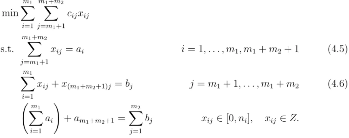
min m1 ∑ i=1 m∑1+m2 j=m1+1 cijxij s.t. m∑1+m2 j=m1+1 xij =ai i= 1, . . . , m1, m1+m2 + 1 (4.5) m1 ∑ i=1 xij +x(m1+m2+1)j =bj j =m1+ 1, . . . , m1+m2 (4.6) (_m 1 ∑ i=1 ai ) +am1+m2+1 = m2 ∑ j=1 bj xij ∈[0, ni], xij ∈Z.

This problem can be solved easily by the same LP method. Although the total operation cost is minimized in the result, this approach does not guarantee that all the districts will maintain a certain level of service. In fact, some districts which are in great need of trucks may even receive no trucks at all in the end, because the dummy supply district dose not exist actually. Hence, their level of service remain the same as that in the beginning. Consider the following example:

There are four districts in the considered area, in which districts 1 and 2 are supply districts, each with the maximum of two trucks to supply, while districts 3 and 4 are demand districts, each with the minimum of four trucks to receive. Table 5.1 lists the unit reallocation cost between districts:

Table 4.1: Unit Reallocation Cost District 3 District 4

District 1 8 3

(34)

Then the problem can be modeled as follows, which dose not have a feasible solution: min 8x13+ 3x14+ 6x23+ 2x24 s.t. 4 ∑ j=3 x1j = 2 4 ∑ j=3 x2j = 2 2 ∑ i=1 xi3 = 4 2 ∑ i=1 xi4 = 4 xij ∈[0, ni], xij ∈Z.

It is easy to ﬁnd that the total demand (4 + 4) is greater than the total supply (2 + 2) in this example. Then we can add a dummy supply, labeled district 5, whose maximum supply is the diﬀerence between the total demand and the total supply. The problem becomes:

min 8x13+ 3x14+ 6x23+ 2x24 s.t. 4 ∑ j=3 x1j = 2 4 ∑ j=3 x2j = 2 4 ∑ j=3 x5j = 4 2 ∑ i=1 xi3+x53= 4 2 ∑ i=1 xi4+x54= 4 xij ∈[0, ni], xij ∈Z.

The optimal solution for this balanced problem is x14= 2 x24= 2 x53 = 4.

(35)

District 1 and 2 will send all their trucks to district 4, because the cost of moving into district 4 is less than that of moving into district 3 in the objective function. As a result, district 3 receives no truck at all actually, since district 5 does not really exist. Therefore, this method may lead to very low level of service in certain districts – district 3 in this example, which is not fair for those districts, and the allocation plan will not be accepted.

To solve this unfairness, we introduce another policy called Fair Allocation. In a Fair Allocation model, the objective remains the same: ﬁnding the best allocation plan that minimize the total reallocation operation cost. However, we restrict each district to maintain the same level of service after reallocation.

Considering the way we calculated the expected number of trucks needed in each district, it is reasonable to deﬁne the level of service as the number of trucks needed to be fully serve a district. Our objective is trying to ﬁnd a reallocation plan, which maintains the same service level for all districts with minimal cost.

Let Ni denote the expected number of trucks needed in district i to fully serve

the district. Recall that ni denotes the number of trucks that district i originally

has.Then, from (3.2), Ni = n ∑ j=1 K ∑ k=1 piklijfj αksj . (4.7)

(36)

of service in district i after reallocation: ∆Ni =ni−Ni (4.8) ∆Ni′ = (ni− ∑ j∈I xij + ∑ j∈I βxji)−Ni. (4.9)

Where I denotes the set of all districts.

Then, the Fair Allocation model can be modeled as follows:

min∑ i∈I ∑ j∈I cijxij s.t. ∆Ni′ = ∆Nj′ for any i, j ∈I (4.10) xij ∈[0, ni], xij ∈Z.

Lemma 1, which argues that a district both sending and receiving trucks is not allowed in an optimal solution, still holds in this Fair Allocation model. The proof is similar as what we did before:

Suppose that a truck is moved from district i to district j and then district j to districtk. The reallocation of one truck incurs the cost of (cij+cjk), decreases service

level by 1 in district i and by (1−β) in district j, and increase service level byβ in district k.

If the truck is moved directly from district i to district k, the associated cost is cik. Districtidecreases level of service by 1 and district k improve its level of service

byβ, while there is no change of service level in district j.

The second policy costs less and performs better or equally in every district com-pared to the ﬁrst policy. Because this argument can be generalized for multiple trucks and multiple districts, the proof is complete.

(37)

With this lemma in mind, we can easily identify another property of an optimal policy for our Fair Allocation model. Let these m districts be ordered according to non-increasing level of service before reallocation, without loss of generality:

∆Nm ≥∆Nm−1 ≥. . .≥∆N1. (4.11)

Let δ denote the fairness level, i.e. ﬁnal level of service that every district reaches after reallocation. We have

δ= (ni− ∑ j∈I xij + ∑ j∈I βxji)−Ni for any i∈I ∑ i∈I δ=∑ i∈I ni− ∑ i∈I ∑ j∈I xij + ∑ i∈I ∑ j∈I βxji− ∑ i∈I Ni δ= ∑ i∈Ini− ∑ i∈INi−(1−β) ∑ i∈I ∑ j∈Ixij m . (4.12)

When β = 1, which means the best reallocation eﬃciency, δ= ∑ i∈Ini− ∑ i∈INi m = ∑ i∈I∆Ni m ;

when β = 0, which means the worst reallocation eﬃciency, δ= ∆N1. Therefore, ∆N1 ≤δ≤ ∑ i∈I∆Ni m ≤∆Nm. (4.13)

Lemma 2 In an optimal reallocation policy, if districtisend trucks to other districts,

then district(i+1)would not receive any trucks. On the other side, if districtj receive

trucks from other districts, then district (j−1) would not send any trucks.

Proof. If district i need to send trucks in optimal reallocation plan, then it can not receive any trucks because of Lemma 1. That means the fairness level

(38)

Also from (4.8),

∆Ni ≤∆Ni+1. (4.15)

From (4.14) and (4.15), we have

δ≤∆Ni+1. (4.16)

Therefore, district i+ 1 should also only send trucks to other districts, otherwise, it will not reach the fairness level.

On the other side, If district j need to receive trucks to reach the fairness level, then it can not send any trucks because of Lemma 1. That means fairness level

δ≥∆Nj. (4.17)

Also from (4.8),

∆Nj ≥∆Nj−1. (4.18)

From (4.17) and (4.18), we have

δ≥∆Nj−1. (4.19)

Therefore, district j −1 should only receive trucks, otherwise, it will not reach the fairness level.

Corollary 1 If the original service level of district i is greater than the fairness level

δ, then it can only send trucks in an optimal reallocation plan; if the original service

level of district j is less than the fairness level δ, then it can only receive trucks in an

(39)

Proof. From Lemma 1, if districtireceive trucks, it can not send trucks at the same time. Therefore, the service level of district i will exceed the fairness level more.

Similarly, if district j send trucks, it can not receive trucks at the same time. Therefore, the service level of districtiwill decrease, and it can not reach the fairness level. This completes the proof.

From Lemma 2 and Corollary 1, there is a certain district i0 that satisﬁes:

(1) For any i≥i0, District i either only sends trucks or dose not receive any

trucks in optimal reallocation policy;

(2) For any j < i0, District j only receives trucks in optimal reallocation policy;

(3) Fairness level δ lies between ∆Ni0 and ∆Ni0−1, that is: ∆Ni0−1 ≤δ≤∆Ni0.

Our solution procedure that will solve the Fair Allocation problem includes the following stages: first, we find the specific district i0 according to the properties of

the model; then we can calculate the fairness level by its deﬁnition; ﬁnally, we solve the integer problem.

Stage One: Find District i0

For any i≥ i0, (∆Ni−δ) denotes the number of trucks that move out of district

i. Then the total number of trucks moving out should be

∑

i0≤i≤m

(∆Ni−δ). (4.20)

(40)

Then the total number of trucks moving in should be 1 β ∑ 1≤j<i0 (δ−∆Nj) (4.21) .

Since the total number of trucks being sent out should equal the total number of trucks being received, we have:

∑ i0≤i≤m (∆Ni−δ) = 1 β ∑ 1≤j<i0 (δ−∆Nj). (4.22)

According to the third property of district i0, we have:

∑ i0≤i≤m (∆Ni−∆Ni0)≤ 1 β ∑ 1≤j<i0 (∆Ni0 −∆Nj), (4.23) and ∑ i0−1≤i≤m (∆Ni −∆Ni0−1)≥ 1 β ∑ 1≤j<i0−1 (∆Ni0−1−∆Nj). (4.24)

Deﬁne N_kout and N_kin as follows:

N_kout = ∑ k≤i≤m (∆Ni−∆Nk), N_kin = 1 β ∑ 1≤j<k (∆Nk−∆Nj). Lemma 3 Nout k decreases in k; Nkin increases in k.

Proof. For any 1 ≤k < m, N_kout = ∑ k≤i≤m (∆Ni−∆Nk) = (∆Nk−∆Nk) + ∑ k+1≤i≤m (∆Ni−∆Nk) = ∑ k+1≤i≤m (∆Ni−∆Nk).

(41)

Since ∆Nk≤∆Nk+1, then (∆Ni−∆Nk)≥(∆Ni−∆Nk) ∑ k+1≤i≤m (∆Ni−∆Nk)≥ ∑ k+1≤i≤m (∆Ni−∆Nk+1) N_kout ≥N_kout₊₁. Therefore,Nout k decreases in k.

On the other hand, for any 1< k≤m,

N_kin₊₁ = 1 β ∑ 1≤j<k+1 (∆Nk+1−∆Nj) = 1 β ( ∑ 1≤j<k (∆Nk+1−∆Nj) + (∆Nk+1−∆Nk) ) Since ∆Nk≤∆Nk+1 and ∆Nk+1−∆Nk ≥0, (∆Nk−∆Nj)≤(∆Nk+1−∆Nj) 1 β ∑ 1≤j<k (∆Nk−∆Nj)≤ 1 β ∑ 1≤j<k (∆Nk+1−∆Nj) 1 β ∑ 1≤j<k (∆Nk−∆Nj)≤ 1 β ( ∑ 1≤j<k (∆Nk+1−∆Nj) + (∆Nk+1−∆Nk) ) 1 β ∑ 1≤j<k (∆Nk−∆Nj)≤ 1 β ∑ 1≤j<k+1 (∆Nk+1−∆Nj) N_kin≤N_kin₊₁. Therefore,Nin

k increases in k. The proof is complete.

With Lemma 3 and (4.23), we have

∑ k≤i≤m (∆Ni−∆Nk)≤ 1 β ∑ 1≤j<k (∆Nk−∆Nj) for any i0 ≤k ≤m. (4.25)

With Lemma 3 and (4.24), we have

∑ k≤i≤m (∆Ni−∆Nk)≥ 1 β ∑ 1≤j<k (∆Nk−∆Nj) for any 1≤k ≤i0−1. (4.26)

(42)

Therefore, we can ﬁnd i0 through the following steps:

Step 0 Set k = 1. Step 1 Calculate Nout

k , Nkin, Nkout+1 and Nkin+1 .

Step 2 Check if Nout

k =Nkin, then i0 =k, STOP;

if N_kout₊₁ =N_kin₊₁, theni0 =k+ 1, STOP;

if N_kout > N_kin and N_kout₊₁ < N_kin₊₁, theni0 =k+ 1, STOP;

otherwise, setk =k+ 1 and go back to Step 1.

Stage Two: Find Fairness Level δ

When we ﬁnd i0, the fairness level δ can be calculated by (4.22):

β ∑ i0≤i≤m (∆Ni−δ) = ∑ 1≤j<i0 (δ−∆Nj) δ = ∑i0−1 j=1 ∆Nj+β ∑m i=i0∆Ni i0−1 +β(m−i0+ 1) . (4.27)

Stage Three: Solve the Fair Allocation Integer Model

The Fair Allocation model becomes

min m ∑ i=i0 i∑0−1 j=1 cijxij s.t. (ni− i0−1 ∑ j=1 xij)−Ni = (nj +β m ∑ i=i0 xij)−Nj for any i0 ≤i≤m, 1≤j < i0 (4.28) xij ∈[0, ni], xij ∈Z.

(43)

Since δ = (ni −

∑i0−1

j=1 xij)−Ni = (nj+β

∑m

i=i0xij)−Nj, then the model can be

written as min m ∑ i=i0 i∑0−1 j=1 cijxij s.t. (ni− i0−1 ∑ j=1 xij)−Ni =δ for any i0 ≤i≤m (4.29) (nj+β m ∑ i=i0 xij)−Nj =δ for any 1≤j < i0 (4.30) xij ∈[0, ni], xij ∈Z. Or min m ∑ i=i0 i∑0−1 j=1 cijxij s.t. i∑0−1 j=1 xij = (ni−Ni)−δ for any i0 ≤i≤m (4.31) m ∑ i=i0 xij = 1 β(δ−(nj−Nj)) for any 1≤j < i0 (4.32) xij ∈[0, ni], xij ∈Z.

The model above dose not have any feasible solution, because integer numbers would never satisfy the non-integer constraints. To solve this problem, we can round the supply constraint (4.31) to be less than a larger integer number but greater than a smaller integer number, and also round the demand constraint (4.32) to be greater

(44)

than a smaller integer number but less than a larger integer number: min m ∑ i=i0 i∑0−1 j=1 cijxij s.t. ⌊(ni −Ni)−δ⌋ ≤ i0−1 ∑ j=1 xij ≤ ⌈(ni−Ni)−δ⌉ for any i0 ≤i≤m (4.33) ⌈1 β(δ−(nj −Nj))⌉ ≥ m ∑ i=i0 xij ≥ ⌊ 1 β(δ−(nj −Nj))⌋ for any 1≤j < i0 (4.34) xij ∈[0, ni], xij ∈Z.

Then, the integer problem becomes a variant of the transportation problem. It can be solved by transforming to a standard transportation problem, according to the method presented by Dahiya and Verma. Therefore, we can solve it similarly as a transportation model.

(45)

Chapter 5

Case Study

This chapter includes an illustration of the mathematical models and solution ap-proaches proposed in the research. The presented problem in this chapter is based on a series of hypothetical storm situations in the seven service regions in central Missouri. Our objective is to determine the best resource (snow removal trucks) re-allocation plan that maintains the same service level for all service regions with the minimal cost.

5.1

Case Background

5.1.1

Overview

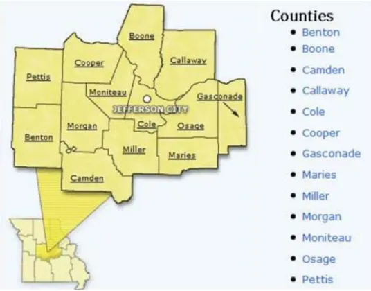
This section provides a case study which motivated this research. As shown in Figure 5.1 and Figure A.1, the area considered for this case study is the seven service regions in Missouri, which include 13 counties, 453,000 people, 7,802 sq. miles and 3,625 road miles to be maintained by Missouri Department of Transportation (MoDOT). As previous mentioned, winter road maintenance work includes the operations of salt and abrasives spreading, snow plowing, loading snow into snow removal vehicles and hauling snow to disposal sites, and presents a variety of decision-making problems, such as routing problem, sector design and ﬂeet sizing, which are extremely complex.

(46)

Therefore, we assume that the winter road maintenance network and policy in each region have been established by a set of predeﬁned routes. The depot location and service range in each district are ﬁxed; the operating and maintenance cost of the snow removal resources is not considered. We focus on the operational objectives and constraints, which are used for the modeling of winter road maintenance resource allocation.

Figure 5.1: Counties in Central Missouri

5.1.2

Winter Road Maintenance Operations

MoDOT conducts three major winter road maintenance operations in the seven dis-tricts: pre-treatment before storm, spreading and plowing during storm, and after-storm cleanup. Pre-treatment operation includes spreading abrasives or chemicals over the roadway in order to prevent formation of ice or pack - snow compacted by

(47)

traﬃc action that becomes nearly as tightly bonded to pavement as ice, before or in the early stages of a storm event. This pre-treatment can be conducted in all types of roadways: highway, bridges, hills and curves. But depending on the storm conditions, it is possible that only part of the roadways need to be pre-treated. Spreading-and-plowing plays the most important role in winter road maintenance operation. Snow plowing operation removes as much snow and loose ice as possible in order to keep the road surface clear, while spreading operation tries to melt ice and improve trac-tion during a storm event in order to keep the road surface from slick. Although the speed of plowing is lower than that of spreading, spreading operation requires more frequent return trips for replenishment than plowing. After-storm cleanup operation is the process of plowing the remaining snow from the roadways. The inner and outer shoulders of highways and major roads need to be served once a storm has ended. Then the remaining snow over any other roadways and bridges which is built up as a result of previous plowing operations can be removed.

5.1.3

Winter Road Maintenance Network

MoDOT is responsible for serving all state roads within the seven districts in the center of Missouri, including interstate highways, state highways and other state roadways. Hence, snow removal vehicles are restricted to the state road network while providing winter road maintenance service.

Since many roadways have multiple lanes and the snow removal vehicle can only serve one pass per lane, we calculate the total service distance of a road with multiple lanes by the multiplication of centerline distance and the number of lanes it has.

(48)

du-ration. For example, interstate highways should be served more often than normal state roadways. According to the survey completed by the managers in major depots, all the state roadways that are served by MoDOT can be classiﬁed based on the his-torical average daily traﬃc (ADT) data. The three-class hierarchy is shown in Table 5.1. Class A1, Class A2 and Class A3 roadways should be served within 2, 6 and 12 hours respectively per 12-hour shift, which means that Class A1, A2 and A3 roadways needs to be served 6, 2, and 1 times respectively per 12-hour shift. The frequency is considered ideal because replenishment and other operational time between service runs are not considered.

Table 5.1: Three-Class Hierarchy

Class ADT

A1 ADT >2500

A2 2500 >ADT > 1000

A3 1000 >ADT

Besides, there are total 37 existing winter road maintenance depots operated by MoDOT within the seven districts in central Missouri. Depot locations and asso-ciated routes have evolved as a result of annual decisions and adjustment made by MoDOT’s managers and planners based on their operational experience. The prox-imity to the highways and other major state roadways, as well as the accessibility to nearby roadways and storage space for maintenance materials and equipment is mostly considered when locating a winter road maintenance depot.

(49)

5.1.4

Winter Road Maintenance Resources

Snow removal vehicles are the most important resources in winter road maintenance operations. There are two types of snow removal vehicles that MoDOT has: heavy-duty single-axle trucks and extra heavy-heavy-duty tandem-axle trucks. The diﬀerence between these two types of vehicles is that the tandem-axle trucks can hold more abrasive or chemical material than the single-axle trucks. Monitors are used in both trucks in order to control the rate of material spreading. Normally, the spreading rate is 200lbs per lane mile, but could increase to 400lbs per lane mile depending on the intensity of the storm. Besides, both could be equipped with 10-, 12-, or 14-foot-wide plow for snow plowing operation. Any of the three types of plow could serve one traﬃc lane by adjusting the angle of the plow, while a larger-size plow would clear the road more thoroughly. The average serving speed is 40 miles per hour on Class A1 roadways, and 30 miles per hour on Class A2 and A3 roadways.

5.2

Model Parameters

5.2.1

Considered Area

We consider the seven service regions in central Missouri determined by MoDOT, and number them from 1 to 7. Each service region may consist of multiple counties. The roadways in each service region can be classiﬁed by the three-class hierarchy which is deﬁned in the last chapter. The service frequency associated with the roadway class is shown in Table 5.2.

The length of a road is deﬁned in lane miles, which means the length of a road with multiple lanes is the product of the centerline distance in a single lane and the

(50)

Figure 5.2: Service Regions in Central Missouri

Table 5.2: Service Frequency by Class

Class ADT Service Frequency per Unit Duration

A1 ADT>2500 6

A2 2500>ADT>1000 2

A3 1000>ADT 1

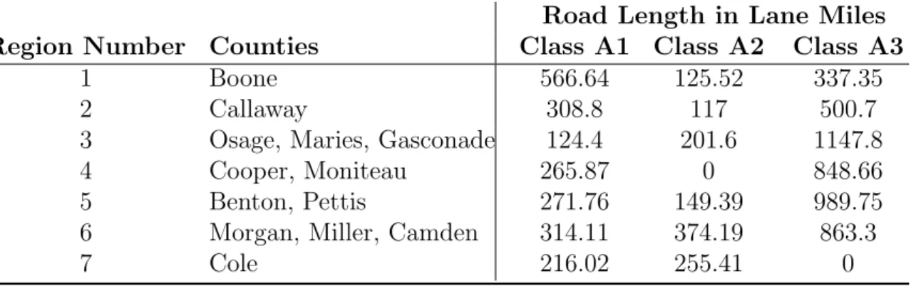
number of lanes it has. Table 5.3 illustrates the road information in each region: Note that since Class A2 roads are mostly scattered in Cole County, we com-bine Class A2 and A3 roads together. Same operation is conducted in Cooper and Moniteau counties.

The distances between service regions are computed by the location of the major depot in each region where the regional supervisor works. All distances between these major depots can be found using the on-line mapping site MapQuest.

(51)

Table 5.3: Roadway Information

Road Length in Lane Miles

Region Number Counties Class A1 Class A2 Class A3

1 Boone 566.64 125.52 337.35

2 Callaway 308.8 117 500.7

3 Osage, Maries, Gasconade 124.4 201.6 1147.8

4 Cooper, Moniteau 265.87 0 848.66

5 Benton, Pettis 271.76 149.39 989.75

6 Morgan, Miller, Camden 314.11 374.19 863.3

7 Cole 216.02 255.41 0

5.2.2

Storm Factors

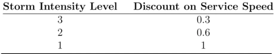
We assume the hypothetical storm has three levels of intensity: from level 1 to level 3. Each storm intensity level has a diﬀerent discount on the normal average service speed of the snow removal vehicle. The greater number indicates the higher intensity of a storm and a lower service speed. As described in table 5.4, in a level 1 storm, snow removal trucks serve the roads at the normal speed, i.e. 40 miles per hour on Class A1 roadways and 30 miles per hour on Class A2 and A3 roadways; while in a level 2 storm, the service speed is reduced to 60% of the normal speed, i.e. 24 miles per hour on Class A1 roadways and 18 miles per hour on Class A2 and A3 roadways; in a level 3 storm, the snow removal trucks can only serve the roads at 30% of the normal speed, that is 12 miles per hour on Class A1 roadways and 9 miles per hour on Class A2 and A3 roadways.

The potential snow storm may have a certain pattern, such as high intensity in the center and low intensity on the edge of the storm. In our case, according to the snowfall 1971-2000 averages data in Appendix C provided by the Midwestern Regional

(52)

Table 5.4: Storm Impact on Service Speed

Storm Intensity Level Discount on Service Speed

3 0.3

2 0.6

1 1

Climate Center, we found that the northeastern part in central Missouri always has much more snowfall than the southwestern part during winter. For example, the annual average snowfall level in Boone and Callaway counties is around 22inches, which is much higher, compared with 11.6inches in Pettis, 5.7inches in Morgan and 11.2inches in Miller. To demonstrate this pattern, we assume that in a hypothetical storm, the probabilities of having high levels of intensities in the northeastern regions, including Callaway and Boone, would be relatively higher, while the probabilities of having high levels of intensities in the southwestern regions, including Cole, Benton, Pettis, Morgan, Miller and Camden, would be relatively lower, and medium in Cooper, Moniteau, Osage, Maries and Gasconade. Therefore, we partition the service regions by the possibilities of having higher levels of storm intensities, however, the value of probability of having each level of storm in a single service region is picked randomly. The illustrations given in this chapter include three scenarios of hypothetical storm situations in central Missouri. In the ﬁrst scenario, the intensity of the hypothetical storm is very weak, and all the service regions have low probabilities of facing high intensity levels. In the second scenario, the intensity of the hypothetical storm is stronger than the ﬁrst one, thus, all the service regions have higher probabilities of facing high intensity levels. In the third scenario, the hypothetical storm becomes very strong, causing the greatest risk of intense storms and need for snow removal

(53)

trucks. Although the intensity of the hypothetical storm changes in each scenario, the same storm pattern holds. That is, in any scenario, the northeastern regions 1 and 2 would have relatively higher probabilities of facing strong storms than others, while the southwestern regions 5, 6 and 7 would have relatively lower probabilities of facing them.

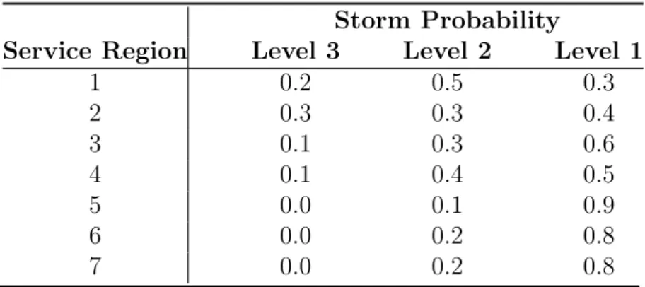
The sets of probabilities of having diﬀerent levels of intensities in each service region for each scenario are shown in the following tables:

Table 5.5: Storm Probabilities in Each Region (Scenario 1) Storm Probability

Service Region Level 3 Level 2 Level 1

1 0.2 0.5 0.3 2 0.3 0.3 0.4 3 0.1 0.3 0.6 4 0.1 0.4 0.5 5 0.0 0.1 0.9 6 0.0 0.2 0.8 7 0.0 0.2 0.8

Service Region Level 3 Level 2 Level 1

1 0.4 0.4 0.2 2 0.5 0.4 0.1 3 0.3 0.4 0.3 4 0.3 0.5 0.2 5 0.0 0.3 0.7 6 0.2 0.3 0.5 7 0.1 0.3 0.6

(54)

Service Region Level 3 Level 2 Level 1

1 0.6 0.3 0.1 2 0.7 0.2 0.1 3 0.4 0.5 0.1 4 0.5 0.4 0.1 5 0.2 0.4 0.4 6 0.3 0.4 0.3 7 0.3 0.3 0.4

5.2.3

Service Resource

Since there is little diﬀerence in service speed and service duration between single-axle trucks and tandem-axle trucks, we consider only one type of trucks. Assume that the vehicle crew could work 8 hour shift a day. Then the service distance for one shift is 320 miles on Class A1 roadways, and 240 miles on Class A2 and A3 roadways.

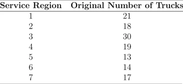
Table 5.8 lists the number of trucks available in each region before reallocation.

Table 5.8: Original Number of Trucks Service Region Original Number of Trucks

1 21 2 18 3 30 4 19 5 13 6 14 7 17

To ﬁnd the reallocation cost, we suppose the MPG of a snow removal truck is 10 miles per gallon, and the gas price is 2.4 dollars per gallon, then the fuel cost is 0.24 dollars per mile. In addition, operating cost, repair cost and depreciation cost are

(55)

considered based on John Siebert’s report ”Truckers must not be ﬂying by the seat of their pants”, which is posted on Owner-Operator Independent Drivers Association Website, and the vehicle replacement cost analysis in Appendix D.

We estimate the total reallocation cost as the total cost of fuel, operating, repair and depreciation, which is (1.2 + 0.24) dollars per mile. We also assume that the reallocation ineﬃciency discount is 0.8, which means the reallocated trucks are only able to complete 80% of the regular workload in the new service region.

5.3

Case Results and Analysis

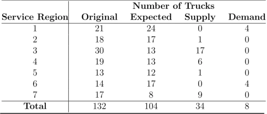
First, we coded the proposed model by Matlab to determine whether feasible solution exists in this problem. The result for each scenario is shown below:

Table 5.9: N