Individual, Aggregate, and Cluster-based Aggregate
Forecasting of Residential Demand
Tri Kurniawan Wijaya, Matteo Vasirani, Samuel Humeau, Karl Aberer
School of Computer and Communication Sciences EPFL, Switzerland
{tri-kurniawan.wijaya, matteo.vasirani, samuel.humeau, karl.aberer}@epfl.ch
ABSTRACT
While the literature has focused on large, industrial, or na-tional demand, this paper focuses on short-term (1 and 24 hour ahead) electricity demand forecasting for residential customers at the individual and aggregate level. Since elec-tricity consumption behavior may vary between households, we first build a feature universe, and then apply Correlation-based Feature Selection to select features relevant to each household. We find that the improvement provided by the Cluster-based Aggregate Forecasting strategy depends not only on the number of clusters, but more importantly on the size of the customer base.
Categories and Subject Descriptors
H.2.8 [Database Management]: Database Applications—
Data mining; G.3 [Probability and Statistics]: Time
se-ries analysis; I.5.3 [Pattern Recognition]: Clustering—
Algorithms
Keywords
electricity load forecasting, clustering, residential, smart me-ters, linear regression, support vector machine, multi-layer perceptron
1.
INTRODUCTION
The exploitation of renewable energy, the integration of dis-tributed energy resources at the distribution level, and the electrification of private transportation are considered as suitable governmental policies to tackle some of the prob-lems of advanced societies, such as reducing CO2 emissions
or increasing energy efficiency [13]. In recent years, these solution concepts started to pose new challenges to the ex-isting power grids, whose hierarchical, centrally-controlled structure has remained unchanged for a century. For exam-ple, the exploitation of renewable sources such as solar or wind may be problematic due to their variable and inter-mittent nature, while the integration of distributed energy
resources may cause congestion and atypical power flows that threaten system’s reliability [29].
In this context, energy consumption prediction for different time horizons (e.g., 1 hour ahead, 1 day ahead, 1 month ahead) and space scales (e.g., distribution transformer, in-dividual house-level meter) is becoming crucial for many applications, such as frequency and voltage regulation, de-mand response (to estimate customer’s baseline [40]), and autonomous emergency management [30]. While long-term load forecasting (1–10 years ahead) is important for plan-ning both, transmission and distribution networks, short-term load forecasting (hours to days ahead) is important for the demand response, online scheduling, and security func-tions of an energy management system. In this paper, we use the termsenergy consumption(ordemand) andload in-terchangeably.
Many techniques for energy consumption prediction have been inspired by research on statistical and machine learn-ing, from Linear Regression [18, 32], ARMA [20, 36], and Generalized Additive Models [6, 12] to Neural Networks [5, 17, 25] and Support Vector Regression [11, 34]. However, these techniques have been typically used at very large space scales, such as predicting the electrical load of a market seg-ment serving thousands of customers or even an entire coun-try.
Overview of Contributions
We summarize our contributions as follows.
• Since energy consumption behavior might vary among households, a feature that are relevant for one house might not be relevant for others. Additionally, we have a large number of houses. Thus, feature selection has to be done automatically. To this end, we first build a (large) feature universe, and then automatically de-termine the relevant features for each house using the Correlation-based Feature Selection [16], which selects subset of features set that are highly correlated with the response variable while having low inter-correlation between each other (see Section 4.1).
• We demonstrate how machine learning algorithms that are typically used to forecast energy demand of large-scale customers can also be used to forecast house-holds’ consumption and improve the benchmark by
around 20%–24% (see Section 4.2 and Section 5). Ad-ditionally, we also compare their performances with that of Seasonal ARIMA (see Appendix). Looking at prediction results, however, load forecasting at the household level remains a hard problem.
• We find that the improvement provided by the Cluster-based Aggregate Forecasting strategy (compared to the traditional aggregate forecasts) depends not only on the number of the clusters, but more importantly on the size of the customer base. That is, the larger the customer base, the higher the improvement (see Section 6.2). Thus, our finding offers additional in-sight to the practitioners who wish to implement this strategy in the real world.
2.
RELATED WORK
Electricity demand forecasting has been widely studied in the literature. In addition to studies that focusing on the forecasting methodology,1researchers have also studied
par-ticular geographical areas or countries [4, 7, 8, 28, 31, 33]. Competitions have also been organized [11, 19]. All of them, however, focused on demand forecasting on a large scale, ei-ther at the regional or national level.
Due to the recent deployment of smart meters, forecasting energy demand at the residential level is a relatively new area. The work by Ghofrani et al. [14] can be considered as one of the earliest works in the field, where they fore-cast the electricity demand of a single household, using one day of training and one day of test data. Our initial work in [21] is one of the first to consider a large set (hundreds to thousands) of households. Since then, some interesting results have been published. Tidemann et al., for example, showed that due to irregularities in electricity demand at the household level, forecasting demand at the household level is indeed more difficult than at the distribution or transmis-sion level [38]. Chaouch used functional wavelet-kernel and then improved it by clustering daily load curves and trained each cluster separately [10]. The approach took only the historical load curve as input, and therefore a careful modi-fication need to be performed to account for external factors, such as calendar variables or temperatures. In contrast, by using machine learning algorithms (such as Linear Regres-sion, Multi-Layer Perceptron, or Support Vector Machine), incorporating new external factors is essentially adding new elements to the feature vector. Thus, as there will be more and more contextual data concerning households available in the future, machine learning algorithms facilitate the seam-less addition of new features.2
Haben et al. proposed theadjusted error measure to toler-ate forecasted values that are slightly misplaced in time [15]. The measure can also be seen as a generalization of the
stan-dard p-norm error. More specifically, when the tolerance
magnitude,w, is equal to zero, the measure reduces to the standardp-norm errors. It is not scale-independent,
how-1We have mentioned the references in Section 1, i.e., Linear
Regression [18, 32], ARMA [20, 36], Generalized Additive Models [6, 12], Neural Networks [5, 17, 25] and Support Vector Regression [11, 34].
2Several works have used demographic information to
esti-mate electricity demand. See, e.g., [24, 26, 28, 39].
ever, which makes it unsuitable to compare or aggregate the accuracy of the demand forecasts of different households. Furthermore, it requires permutation of the forecasts, and thus needs cubic time to compute, whereas most evaluation metrics takes only linear time.
Misiti et al. [27] studied the effect of forecasting clusters of industrial customers to predict their aggregate demand using wavelet-based clustering.3 Alzate and Sinn [3] used kernel spectral clustering and consider a mix of residential customers and small/medium enterprises. Interestingly, al-though [3, 27] and our work focus on different customer bases and use different forecasting and clustering algorithms, all conclude that clustering customers and then forecasting each cluster separately could indeed improve aggregate fore-casts. We continue by investigating how the improvement provided by this Cluster-based Aggregate Forecasting strat-egy depends not only on the number of clusters, but also on the size of the customer base (Section 6.2). Additionally, compared to [3, 27], our clustering objective is clear, target-ing a specific property of the resulttarget-ing cluster (Section 6.1).
3.
DATASET AND EVALUATION METRICS
3.1
Dataset
We use the detailed data underlying electricity consumption behaviour provided in anonymized format by the Commis-sion for Energy Regulation (CER) in Ireland.4 This dataset
is the result of the Electricity Customer Behaviour Trials (CBTs), which took place during 2009 and 2010 with over 5,000 Irish homes and businesses participating. The partici-pants in the trials had an electricity smart meter installed in their homes/premises, which collected energy consumption measurements (in kWh) every half hour. The objective of the trial was evaluating the impact that different Time-Of-Use (TOU) tariffs have on the consumption behaviour. Although the CER has carefully cleaned the data (e.g., mul-tiple imputation for the missing values—see [37] Appendix 2), there are still a small number of missing values found in the dataset. In this work, unless stated otherwise, we choose customers who have no missing values in their mea-surements. Furthermore, to avoid bias due to the TOU tar-iffs, we consider only the residential households in the control group of the trial, i.e.
”those customers with a flat rate that did not change their consumption behavior in response to a TOU tariff. This results in the selection of 782 customers. The measurements are aggregated into hourly timeslots. For all results presented in this paper, we use the first year (from July 2009 to June 2010) as the training set, and the remain-ing 6 months (from July 2010 to December 2010) as the test set.
3.2
Evaluation metrics
In the literature, there are three widely used metrics to eval-uate the accuracy of a forecasting algorithm: the Mean Ab-solute Percentage Error (MAPE), the Mean AbAb-solute Error
3They refer to this approach asdisaggregated load forecast-ing. To avoid confusion with the individual load forecast-ing, we use the term Cluster-based Aggregate Forecasting instead.
4http://www.ucd.ie/issda/data/
(MAE), and the Root Mean Square Error (RMSE). Given a time seriesS ={s1, s2, . . . , sn}of observed consumption
values and the estimation produced by forecasting algorithm
b
S={bs1,bs2, . . . ,sbn}, the MAPE is defined as:
MAPE(S,Sb) = 1 n n X t=1 st−bst st (1) The MAPE is a quite intuitive metric. However, it has a ma-jor drawback, i.e., it is not robust to the division by values approaching zero. Many households in the dataset have zero consumption on certain time slots, which makes the MAPE undefined, Furthermore, it is quite common to have house-holds with very small consumption values, which makes the MAPE very large, approaching infinity.
Unlike the MAPE, the MAE and the RMSE do not suffer from the division by values approaching zero, since the MAE is defined as MAE(S,Sb) = 1 n n X t=1 (st−sbt), (2)
and the RMSE is defined as
RMSE(S,Sb) = v u u t 1 n n X t=1 (st−bst)2. (3)
However, they are scale-dependent metrics. Since the aver-age hourly consumption of households in the dataset varies between 0.05 kWh and 3.83 kWh, we need scale-independent metrics to aggregate the forecasting error of these differ-ent households. Moreover, scale-independdiffer-ent metrics can be useful to compare not only the forecasting error of different households, but also the forecasting error of different tem-poral aggregations or consumer groups.5
To this end, we suggest to use other metrics that are both, scale-independent, and robust to the division by values ap-proaching zero, namely the Normalized Mean Absolute Er-ror (NMAE) and the Normalized Root Mean Square ErEr-ror (NRMSE). The NMAE is defined as
NMAE(S,Sb) = MAE(S,Sb) ||S||1 = n X t=1 |st−bst| n X t=1 |st| , (4) and the NRMSE is defined as
NRMSE(S,Sb) = RMSE(S,Sb) ||S||2 = v u u t n X t=1 (st−bst) 2 n X t=1 s2 t . (5) While one zero measurement is enough to make the MAPE
5
Apart from MAPE, MAE, and RMSE, there are also other options, such as theadjusted error[15] and the MASE [23]. See Section 2 for the discussion about the adjusted error
and the supplementary material [1] for the discussion about MASE.
undefined (or approaches infinity), all measurements need to be zero to make the NMAE or the NRMSE undefined.
4.
FORECASTING MODELS
4.1
Features
There are two important challenges in selecting features for residential electricity load forecasting. First, different houses might have different energy consumption behavior. Thus, features that are relevant to one house might not be relevant to other houses. Second, we have a large number of houses. Therefore, feature selection should be done automatically. To solve both challenges, we first build a (large) feature uni-verse and then apply a feature selection algorithm to select features that are relevant to each house. We consider both, historical load and contextual features. To forecast the load at time (or hour) t, for 1 hour ahead forecasting, we con-sider the historical load data from timet−1 tot−336, i.e.,
{st−1, st2, . . . , st−336}. 6
While for 24 hour ahead forecast-ing, we consider the historical load data from time t−24 tot−336 (since the historical load data from timet−1 to
t−23 is not available in this case).
The CER dataset does not contain any information about the house or the persons who live in the house. Thus, for contextual features, we consider day of week, hour of day, and weather information. Since there is no information about the city/location of each house, we crawl the histor-ical weather data of the three biggest cities in Ireland, i.e., Dublin, Cork, and Limerick.7 We use 48 hours historical
temperature and humidity data,8 from timet−1 tot−48 for 1 hour ahead forecasting, and from timet−24 tot−71 for 24 hour ahead forecasting. Additionally, we also use in-clude the mean and the median of those three cities to the feature set.
Up to this point, our feature universe contains approxi-mately 800 variables. Next, we apply Correlation-based Feature Selection (CFS) to each house. This method se-lects subset of features that are highly correlated with the response variable while having low inter-correlation between each other [16]. As a result, we obtain a (much) reduced subset of relevant features for each house.
4.2
Learning Algorithms
Various learning algorithms have been used to forecast large-scale electricity demand. Recent literature suggests Support Vector Regression (SVR) as one of the most effective models to forecast future energy consumption [11, 34]. Other well established methods are Linear Regression and Multi-Layer Perceptron (MLP). In this section, we briefly describe our model setup.
4.2.1
Linear Regression configuration
A linear model to predict the load at timetis defined as:
6
Of course, longer time duration can also be considered here, in the price of memory and computation cost.
7
We obtained the weather-related data from http://www. wunderground.com.
8
Apart from temperature, humidity has also been used in real-world implementation to forecast electricity demand. See, e.g., [2].
0.55 0.56 0.57 0.58 1 2 3 NRM SE # hidden layers α=0.3 α=0.1
Figure 1: MLP model evaluation (using NRMSE) using dif-ferent number of hidden layers and learning ratesαon ran-domly chosen 25 households. The lower the better. In the end, we use one hidden layer andα= 0.1.
y=θTx+ (6)
whereθis the vector of coefficients,xis the feature vector, andis the error term. We estimate the coefficients and the error term of the linear model using ridge regression (other methods, of course, can also be used).
4.2.2
MLP configuration
We use one hidden layer with sigmoid activation functions. The output can be written asy=W2×Θ(W1·x+B1)+B2
wherexis the input vector,yis the output value,W1,W2,
B1, andB2 are the coefficient matrices, and Θ is the
sig-moid operator. Each componentxjof the input vectorxis
standardized, i.e.,x∗j = (xj−µj)/σj, whereµjis the mean
andσjis the standard deviation of the values in thejth
di-mension. To avoid overfitting, a validation set is constructed by randomly selecting 30% of the instances in the training set. The coefficient matrices are learnt using gradient de-scent, with learning rate ofα = 0.1 (see the evaluation of different hidden layers and learning rates in Figure 1). The stopping criterion is triggered when the error on the valida-tion set (calculated after each epoch) has increased 20 times in a row.
4.2.3
SVR configuration
SVR is a regression method based on Support Vector Ma-chine (SVM) that has been developed in 1996 by Vapnik (see also the tutorial by Smola and Schlkopf [35]). In this work, we use the SVR implementation provided by the LIBSVM library developed by Chang and Lin [9].
SVR must be provided with the SVM error cost C and a kernel function. For the kernel function, we use the RBF kernel, similar to [11]. Next, to find suitable values forCand
γ, we split the training set into two parts: a sub-training set and a validation set. The SVR is trained on the sub-training set, and evaluated on the validation set. ForCwe test a set of values{1,10,102,103,104,105}, while forγ we test a set
of values{0,0.01,0.1,1}.
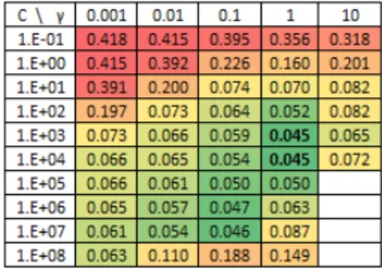
For individual load forecasting, we find that different val-ues ofC and γ do not result in significant NRMSE differ-ences (see Figure 2a and 2b) . However, they strongly affect the computation time, which dramatically increase when
(a) (b)
(c)
Figure 2: SVR model evaluation for individual forecasting on the randomly chosen 25 households: (a) average NRMSE on the validation set given differentC andγ, (b) standard deviation on the average, (c) average running time. The lower the better. In the end, we choose C= 100 and γ = 0.01. While there are some other settings which yield better NRMSE, they typically require considerably longer running time.
Figure 3: SVR model evaluation (measured by average NRMSE) for aggregate forecasting. The lower the better.
C ≥ 1000 or γ ≥ 0.1 (see Figure 2c). Thus, for individ-ual forecast, we use C = 100 andγ = 0.01. On the other hand, for aggregate forecast, different settings of C and γ
result in significant differences in terms of NRMSE (see Fig-ure 3). We found that C = 1000 and γ = 1 is the best setting.
5.
INDIVIDUAL FORECASTING
In addition to features and learning algorithms, we also ex-plorepth root transformation. That is, instead of modeling the response variable (st) as is, we model itspth root (s
1/p t ),
and then transform the forecasted value back to its original dimension by raising it to the pth power ((bst)p). Since the
distribution of household energy consumption are skewed to the left toward zero,pth root transformation could help to make it more normal and easier to model.
Tables 1 and 2 show the performance of Linear Regression (LR), Multi-Layer Perceptron (MLP), and Support Vector Re-gression (SVR) using the setting described in Section 4. Both tables show that the pth root transformation mostly im-proves the NMAE of the models. Additionally, as a
compar-(a) Aggregate consumption (782 households).
(b) Example consumption of a household (id 1002). Figure 4: A sample of hourly energy consumption from the CER dataset, from Monday, 07 to Sunday, 2009-09-13.
ison to the three models above, we usepersistence forecast
as the benchmarks, i.e., the load of the previous hour (st−1)
for the 1 hour ahead forecasting, and the load for the same hour of the previous day (st−24) for the 24 hour ahead
fore-casting. Although household-level forecasting is a difficult problem, we show that it is possible to improve the pre-diction by around 20% – 24% compared to the benchmark. Moreover, the improvements provided by the three learning algorithms for the 24 hour ahead forecasting are consistently higher than that of 1 hour ahead, which shows the greater advantage of using the learning algorithms (rather than the benchmarks) on a longer forecasting horizon.
6.
AGGREGATE FORECASTING
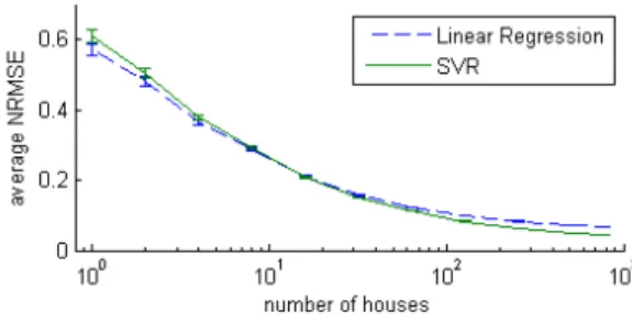
In order to provide an aggregate forecast of a set of individually-monitored households, it is possible to define two extreme strategies: (1) aggregate the energy consumption of all house-holds into one time series (the aggregate consumption), then forecast the aggregate consumption, and (2) forecast the en-ergy consumption of each household separately, then aggre-gate the forecasts. Since the patterns in aggreaggre-gate consump-tion are more regular than that of individual consumpconsump-tion (see also Figure 4), intuitively, strategy (1) should outper-form strategy (2). Figure 5 shows clearly that the forecasting error decreases as the aggregation size increases.
In this section, we evaluate an alternative strategy (3), where we segment the households into k clusters, aggregate the energy consumption of the households in each cluster, fore-cast each cluster separately, and finally aggregate thek fore-casts into one aggregate forecast. Strategy (1) and (2) can also be seen as some special cases of strategy (3), where
k= 1 andk=N = total customers, respectively. We refer to strategy (3) as the Cluster-based Aggregate Forecasting (CBAF). The contributions of this section are: (i) we pro-vide clustering algorithms to form clusters with some pre-defined/targeted characteristics (see Section 6.1), whereas previous works offer only little interpretation to the
char-Figure 5: The NRMSE of LRandSVRfor 1 hour ahead fore-casting (the lower the better). Forefore-casting error decreases as the aggregation size increases.
acteristics of the resulting clusters, (ii) we find that the im-provement provided by the CBAF strategy depends not only on the number of clusters, but also on the size of the cus-tomer base (see Section 6.2).
6.1
Clustering algorithms
In order to investigate the effectiveness of CBAF, we define several clustering methods with clear objective, targeting a specific property of the resulting clusters:
• Max-AC: This method aims to maximize the auto-correlation of the energy consumption of the clusters. More specif-ically, this method uses the greedy clustering technique proposed in Algorithm 1 to find clusters such that the auto-correlation of the load of each cluster is maxi-mized. Letac(S) be the average auto-correlation (up to a certain lag) of time series S.9 In addition, we
define acluster as a set of customers, and Sc as the
aggregate consumption time series of clusterc. Then this method uses Algorithm 1 by defining
Φ(c, x) =ac(Sc∪{x})−ac(Sc),
wherexis a customer. As a consequence, customerx
is assigned to a cluster where xprovides the highest improvement to the auto-correlation of the clusters’ energy consumption.
• Min-Stdev: This method aims to minimize the fluctu-ation in the clusters’ energy consumption, which often becomes the main challenge to predict. In particular, it aims to minimize the standard deviation of the clus-ters’ energy consumption. Letsd(S) be the standard deviation of time seriesS. As in theMax-AC case, we define a cluster as a set of customers, and Sc as the
aggregate consumption time series of clusterc. Then this method uses Algorithm 1 by defining
Φ(c, x) = (sd(Sc)−sd(Sc∪{x}))· |c|,
where x is a customer. As a consequence, customer
xis assigned to a cluster wherexminimizes the stan-dard deviation of the cluster’s aggregate consumption. Note that in the evaluation function Φ, we multiply the standard deviation difference by|c|so as to have
9
In our implementation, we compute the auto-correlation up to lag 168 (or, 1 week preceding the target time). Other lags, however, can also be used.
Table 1: Average NRMSE and NMAE (with its 95% confidence interval) ofLR,MLP,SVRfor 1 hour ahead load forecasting at the level of the individual customer. Benchmark (bm) isst−1. The numbers in parentheses show the improvements compared
to the benchmark. Root transformation (st1/p, withp >1) can be used to improve NMAE.
p= 1 p= 2 p= 4 N RM S E bm 0.694±0.010 0.694±0.010 0.694±0.010 LR 0.557±0.007 (19.7%) 0.562±0.007 (19.1%) 0.571±0.007 (17.7%) MLP 0.575±0.008 (17.2%) 0.569±0.007 (18.1%) 0.578±0.008 (16.6%) SVR 0.573±0.008 (17.4%) 0.571±0.007 (17.8%) 0.572±0.007 (17.6%) N M AE bm 0.562±0.010 0.562±0.011 0.562±0.011 LR 0.495±0.009 (11.9%) 0.461±0.007 (17.9%) 0.456±0.007 (18.9%) MLP 0.535±0.014 (4.7%) 0.477±0.009 (15.0%) 0.468±0.008 (16.7%) SVR 0.461±0.007 (17.9%) 0.448±0.007 (20.2%) 0.452±0.007 (19.5%)
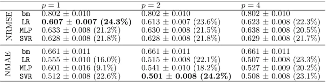
Table 2: Average NRMSE and NMAE (with its 95% confidence interval) ofLR,MLP,SVRfor 24 hour ahead load forecasting at the level of the individual customer. Benchmark (bm) isst−24. The numbers in parentheses show the improvements compared
to the benchmark. Root transformation (st1/p, withp >1) can be used to improve NMAE.
p= 1 p= 2 p= 4 N RM S E bm 0.802±0.010 0.802±0.010 0.802±0.010 LR 0.607±0.007 (24.3%) 0.613±0.007 (23.6%) 0.623±0.008 (22.3%) MLP 0.633±0.008 (21.2%) 0.630±0.008 (21.5%) 0.638±0.008 (20.5%) SVR 0.628±0.008 (21.8%) 0.628±0.008 (21.8%) 0.629±0.008 (21.7%) N M AE bm 0.661±0.011 0.661±0.011 0.661±0.011 LR 0.555±0.010 (16.0%) 0.515±0.008 (22.1%) 0.507±0.008 (23.3%) MLP 0.601±0.016 (9.1%) 0.541±0.010 (18.2%) 0.527±0.009 (20.2%) SVR 0.512±0.008 (22.6%) 0.501±0.008 (24.2%) 0.508±0.008 (23.1%)
Algorithm 1:Generic greedy clustering algorithm
Input: number of clustersk, customer setX
Output: cluster configurationC={c1, . . . , ck}
1 {x1, . . . , xk} ←draw randomlykcustomers fromX
2 fori∈ {1, . . . , k}do ci←xi /*initialization*/
3 whileX6=∅do
4 x←draw randomly a customer fromX
5 c∗←arg maxc∈CΦ(c, x)
6 c∗←c∗∪ {x}
7 returnC
a weighted difference, with respect to the size of the original clusterc(beforexis added).
• Max-Sim: This method aims to maximize the similarity among customers within a cluster. Unlike previous two methods, here we apply KMeans clustering algorithm to customer’s 24-hour load profiles, where each hour is characterized by the distribution (or histogram) of the amount of energy consumed in that hour. More specifically, for each hour, we define a feature vector of length 21. For the first 20 elements, theith element is the frequency of consumption between (i−1)×0.5 kWh andi×0.5 kWh. The 21stelement is the frequency of consumption greater than 10 kWh. Finally, we apply KMeans on the customers’ feature vectors, where each feature vector of a customer is of length 24×21 = 504.
• Random: Each customer is randomly assigned to any of the clusters with the equal probability.
In this experiment, we enlarge our dataset to include all res-idential customers who have no missing values. This results
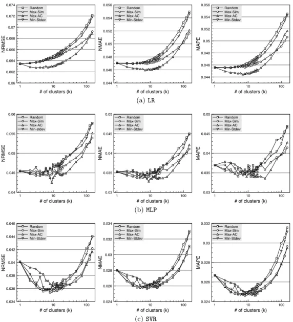
in the selection of 3,639 customers. Figures 6 shows the NRMSE, the NMAE and the MAPE ofLR,MLPandSVR, for a different number of clustersk. Whenk= 1, all customers are aggregated into a single cluster and a single prediction is performed. Ask increases, more clusters are created (k
clusters to be precise), and the consumption of each cluster is forecasted separately. The forecasts are then aggregated into a single aggregate forecast. Note that,k= 1 represents strategy (1), k =N = 3639 strategy (2), and 1 < k < N
the CBAF strategy, which is the focus of this section. We do not show the forecasting result beyond k = 128 as the error continues to increase beyond that of k= 1. This fact clearly shows that, strategy (1) outperforms strategy (2). Additionally, there are some 1< k < N for which the fore-casting error is lower than that ofk= 1. This fact confirms that CBAF indeed can be used to improve the accuracy of aggregate forecasting.
Interestingly, all clustering methods that we introduced (in-cludingRandom) seem to be able to provide a lower forecast-ing error than that of strategy (1). Although in some cases Max-AC provides the lowest error curve as it aims to maxi-mize the auto-correlation of the energy consumption within the clusters,10the accuracies of these clustering methods are often marginally different. Therefore, choosing one cluster-ing method against the others (or implementcluster-ing the CBAF strategy) in a real-world scenario needs a more careful anal-ysis, in the sense that we need to consider whether the ad-vantage brought by a particular clustering method is greater than the cost of implementing it.
10
Time series with higher auto-correlation is typically easier to forecast since it shows greater relationship between the current and the past values.
1 10 100 # of clusters (k) 0.06 0.062 0.064 0.066 0.068 0.07 0.072 0.074 N R MSE Random Max-Sim Max-AC Min-Stdev 1 10 100 # of clusters (k) 0.044 0.046 0.048 0.05 0.052 0.054 0.056 N MAE Random Max-Sim Max-AC Min-Stdev 1 10 100 # of clusters (k) 0.044 0.046 0.048 0.05 0.052 0.054 0.056 MAPE Random Max-Sim Max-AC Min-Stdev (a)LR 1 10 100 # of clusters (k) 0.04 0.045 0.05 0.055 0.06 N R MSE Random Max-Sim Max-AC Min-stdev 1 10 100 # of clusters (k) 0.03 0.035 0.04 0.045 0.05 N MAE Random Max-Sim Max-AC Min-Stdev 1 10 100 # of clusters (k) 0.03 0.035 0.04 0.045 0.05 MAPE Random Max-Sim Max-AC Min-Stdev (b)MLP 1 10 100 # of clusters (k) 0.034 0.036 0.038 0.04 0.042 0.044 0.046 N R MSE Random Max-Sim Max-AC Min-Stdev 1 10 100 # of clusters (k) 0.024 0.026 0.028 0.03 0.032 0.034 N MAE Random Max-Sim Max-AC Min-Stdev 1 10 100 # of clusters (k) 0.024 0.026 0.028 0.03 0.032 MAPE Random Max-Sim Max-AC Min-Stdev (c)SVR
Figure 6: The NRMSE, the NMAE and the MAPE for a different number of clustersk(the lower the better). Total number of customers,N= 3639. The best accuracy is obtained when 1< k <3639, which shows the effectiveness of CBAF.
6.2
The Impact of the Size of the Customer
Base
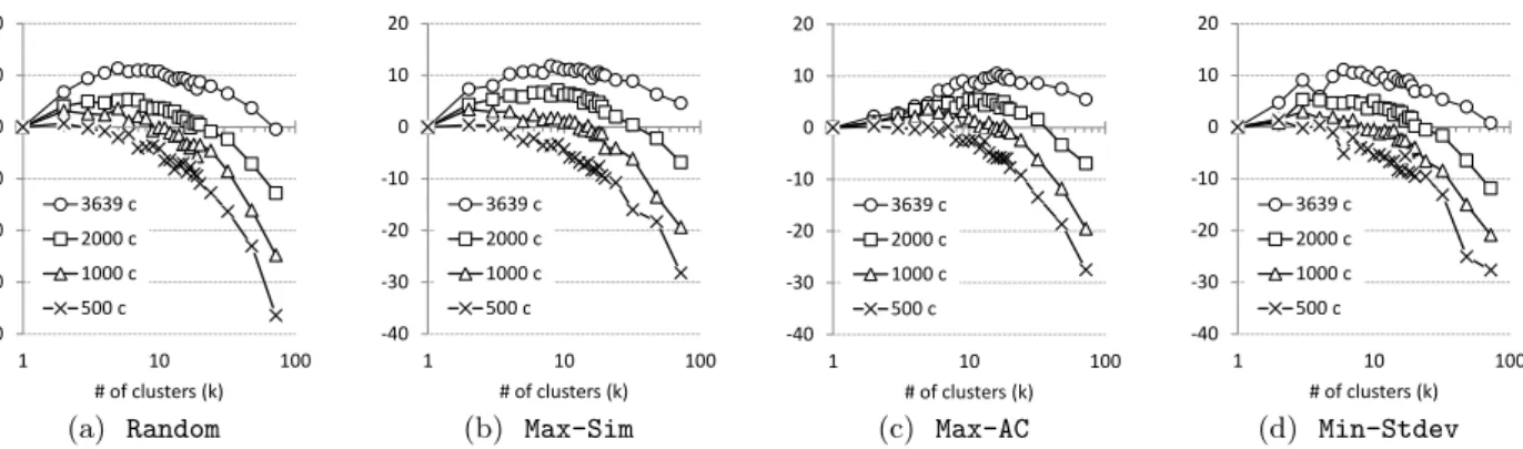
Hitherto one might think that the improvement obtained by CBAF depends on the number of clusters, k. While this insight has been confirmed by Figure 6, there is more to it than that since it turned out that the size of the customer base also plays an important role in the improvement. We repeat the experiments using different sized customer bases: 500, 1,000, and 2,000 (drawn randomly from the original dataset of 3,639 customers). Note that, for the samek, a different size of customer bases implies different cluster sizes. Figure 7 shows the improvement gained bySVRwhen we per-form CBAF on different size of customer bases. While there is almost no positive improvement in the case of 500 cus-tomers (no matter which clustering method is used), some improvement may be noticed in the case of 1,000 customers or more. In general, the improvement increases with the size
of the customer base.
If we assume that a “good” forecast models the true obser-vation and a white noise (zero mean and finite variance), then it means that combining several good forecasts from several clusters into one aggregate forecast could neutralize the white noise. Thus, there is a trade-off between the size and the number of clusters. The size of the clusters should be big enough for the algorithm to deliver a reasonably good prediction,11but not too big that there are not enough clus-ters (hence, predictions) to cancel out the noise.
In addition, since the number of clusters, k, strongly influ-ence the cluster size, one might wonder whether it is possible to set a priori the best value fork. Because characteristics of a customer base vary from one to another, the right k
11See also Figure 5 about the relation between forecast
-40 -30 -20 -10 0 10 20 1 10 100 # of clusters (k) 3639 c 2000 c 1000 c 500 c (a) Random -40 -30 -20 -10 0 10 20 1 10 100 # of clusters (k) 3639 c 2000 c 1000 c 500 c (b) Max-Sim -40 -30 -20 -10 0 10 20 1 10 100 # of clusters (k) 3639 c 2000 c 1000 c 500 c (c) Max-AC -40 -30 -20 -10 0 10 20 1 10 100 # of clusters (k) 3639 c 2000 c 1000 c 500 c (d) Min-Stdev
Figure 7: Percentage improvement in the NRMSE of the CBAF strategy (compared to the traditional aggregate forecast,
k= 1) of 500, 1,000, 2,000, and 3,639 customers over a different number of clusters and clustering methods (the higher the better). The larger the customer set, the higher the improvement gained by CBAF.
should be determined using cross validation on the train-ing set. Apart from that, the experiment suggests that the improvement offered by CBAF will increase further as we in-corporate more and more customers (due to the possibility to increase both, the number and the size of the clusters).
7.
DISCUSSION AND CONCLUSION
In this paper we evaluated different machine learning al-gorithms (LR,MLP, andSVR) for short-term individual and aggregate forecasting (1 hour and 24 hour ahead) of res-idential electricity consumption. Additionally, to measure the forecasting accuracy at the household level effectively, we use evaluation metrics that are scale-independent and robust to values approaching zero, namely the NRMSE and the NMAE.
Individual forecasting, in general, is a challenging task (with NRMSE around 0.6 and NMAE around 0.4–0.5). Aggregate forecasting, however, have better accuracy (with NRMSE around 0.04 and NMAE around 0.03). While in individual forecasting we improve the benchmark by around 20%, using similar techniques, in aggregate forecasting we improve the benchmark by around 74%–78% (NRMSE and NMAE of the benchmark in aggregate forecasting are 0.156 and 0.130 respectively).
AlthoughMLPandSVRare more sophisticated thanLR, in in-dividual forecasting, their forecasting performances are not significantly better thanLR(especially withpth root trans-formation, wherep= 2 orp= 4). In aggregate forecasting, however, SVR is significantly better than LR (see, e.g, Fig-ure 6 wherek= 1). Therefore, in a real-world scenario, one should consider the trade-off between the advantage brought by a more sophisticated model and the cost to implement and maintain it.
In addition, we proposed a generic algorithm to segment customers according to a predefined/targeted objective. We showed its usefulness by forming clusters that (1) maximize the auto-correlation and (2) minimize the standard devia-tion of the clusters’ energy consumpdevia-tion. Addidevia-tionally, we found that the improvement provided by the CBAF strat-egy depends not only on the number of clusters, but also on the size of customer base. More specifically, CBAF
im-proves traditional aggregate forecasting when the size of the customer base is above a certain threshold. Conversely, no improvement is achieved when the size of the customer base is below this threshold, no matter which clustering meth-ods is applied. In general, however, the larger the size of the customer base, the higher the improvement offered by CBAF.
8.
REFERENCES
[1] Supplementary material.http://bit.ly/1yGlqpe. [2] PJM Empirical Analysis of Demand Response
Baseline Methods. White Paper, Apr. 2011. [3] C. Alzate and M. Sinn. Improved electricity load
forecasting via kernel spectral clustering of smart meters. InIEEE 13th International Conference on
Data Mining (ICDM), pages 943–948, Dec 2013.
[4] H. A. Amarawickrama and L. C. Hunt. Electricity demand for Sri Lanka: A time series analysis.Energy, 33(5):724 – 739, 2008.
[5] N. An, W. Zhao, J. Wang, D. Shang, and E. Zhao. Using multi-output feedforward neural network with empirical mode decomposition based signal filtering for electricity demand forecasting.Energy, 49(0):279 – 288, 2013.
[6] A. Ba, M. Sinn, Y. Goude, and P. Pompey. Adaptive learning of smoothing functions: Application to electricity load forecasting. In P. L. Bartlett, F. C. N. Pereira, C. J. C. Burges, L. Bottou, and K. Q. Weinberger, editors,NIPS, pages 2519–2527, 2012. [7] V. Bianco, O. Manca, and S. Nardini. Electricity
consumption forecasting in Italy using linear regression models.Energy, 34(9):1413 – 1421, 2009. [8] J. R. Cancelo, A. Espasa, and R. Grafe. Forecasting
the electricity load from one day to one week ahead for the Spanish system operator.International Journal
of Forecasting, 24(4):588 – 602, 2008.
[9] C.-C. Chang and C.-J. Lin. LIBSVM: A library for support vector machines.ACM Transactions on
Intelligent Systems and Technology, 2:27:1–27:27,
2011.
[10] M. Chaouch. Clustering-based improvement of nonparametric functional time series forecasting: Application to intra-day household-level load curves.
IEEE Transactions on Smart Grid, 5(1):411–419, Jan 2014.
[11] B.-J. Chen, M.-W. Chang, et al. Load forecasting using support vector machines: A study on EUNITE competition 2001.IEEE Transactions on Power
Systems, 19(4):1821–1830, 2004.
[12] S. Fan and R. Hyndman. Short-term load forecasting based on a semi-parametric additive model.IEEE
Transactions on Power Systems, 27(1):134–141, Feb
2012.
[13] C. W. Gellings.The Smart Grid: Enabling energy
efficiency and demand response. The Fairmont Press,
Inc., 2009.
[14] M. Ghofrani, M. Hassanzadeh, M. Etezadi-Amoli, and M. Fadali. Smart meter based short-term load forecasting for residential customers. InNorth
American Power Symposium (NAPS), pages 1–5, Aug
2011.
[15] S. Haben, J. Ward, D. V. Greetham, C. Singleton, and P. Grindrod. A new error measure for forecasts of household-level, high resolution electrical energy consumption.International Journal of Forecasting, 30(2):246 – 256, 2014.
[16] M. A. Hall.Correlation-based feature selection for
machine learning. PhD thesis, The University of
Waikato, 1999.
[17] H. S. Hippert, C. E. Pedreira, and R. C. Souza. Neural networks for short-term load forecasting: A review and evaluation.IEEE Transactions on Power
Systems, 16(1):44–55, 2001.
[18] T. Hong.Short-Term Electric Load Forecasting. PhD thesis, North Carolina State University, Sept. 2010. [19] T. Hong, P. Pinson, and S. Fan. Global energy
forecasting competition 2012.International Journal of
Forecasting, 30(2):357 – 363, 2014.
[20] S.-J. Huang and K.-R. Shih. Short-term load forecasting via ARMA model identification including non-gaussian process considerations.IEEE
Transactions on Power Systems, 18(2):673–679, May
2003.
[21] S. Humeau, T. K. Wijaya, M. Vasirani, and K. Aberer. Electricity load forecasting for residential customers: Exploiting aggregation and correlation between households. InSustainable Internet and ICT for
Sustainability (SustainIT), 2013, pages 1–6, Oct 2013.
[22] R. J. Hyndman and Y. Khandakar. Automatic time series forecasting: The forecast package for R.Journal of Statistical Software, 27(3):1–22, 7 2008.
[23] R. J. Hyndman and A. Koehler. Another look at measures of forecast accuracy.International Journal of Forecasting, 22(4):679ˆa ˘A¸S–688, 2006.
[24] A. Jarrah Nezhad, T. K. Wijaya, M. Vasirani, and K. Aberer. SmartD: Smart Meter Data Analytics Dashboard. InThe 5th ACM International Conference
on Future Energy Systems (e-Energy’14), 2014.
[25] A. Khotanzad, R. Afkhami-Rohani, T.-L. Lu, A. Abaye, M. Davis, and D. Maratukulam. ANNSTLF-A Neural-Network-based Electric Load Forecasting System.IEEE Transactions on Neural
Networks, 8(4):835–846, Jul 1997.
[26] J. Z. Kolter and J. Ferreira. A large-scale study on
predicting and contextualizing building energy usage. In W. Burgard and D. Roth, editors,AAAI. AAAI Press, 2011.
[27] M. Misiti, Y. Misiti, G. Oppenheim, and J.-M. Poggi. Optimized clusters for disaggregated electricity load forecasting.REVSTAT, 8:105–124, 2010.
[28] Z. Mohamed and P. Bodger. Forecasting electricity consumption in New Zealand using economic and demographic variables.Energy, 30(10):1833 – 1843, 2005.
[29] A. Mohd, E. Ortjohann, A. Schmelter, N. Hamsic, and D. Morton. Challenges in integrating distributed energy storage systems into future Smart Grid. In
IEEE International Symposium on Industrial
Electronics, pages 1627–1632, June 2008.
[30] K. Moslehi and R. Kumar. A reliability perspective of the Smart Grid.IEEE Transactions on Smart Grid, 1(1):57–64, June 2010.
[31] H.-T. Pao. Comparing linear and nonlinear forecasts for Taiwan’s electricity consumption.Energy, 31(12):2129 – 2141, 2006.
[32] A. Papalexopoulos and T. Hesterberg. A
regression-based approach to short-term system load forecasting.IEEE Transactions on Power Systems, 5(4):1535–1547, Nov 1990.
[33] S. Saab, E. Badr, and G. Nasr. Univariate modeling and forecasting of energy consumption: the case of electricity in Lebanon.Energy, 26(1):1 – 14, 2001. [34] N. Sapankevych and R. Sankar. Time series prediction
using support vector machines: A survey.IEEE
Computational Intelligence Magazine, 4(2):24 –38,
May 2009.
[35] A. J. Smola and B. Sch¨olkopf. A tutorial on support vector regression.Statistics and Computing,
14(3):199–222, Aug. 2004.
[36] J. W. Taylor. Triple seasonal methods for short-term electricity demand forecasting.European Journal of
Operational Research, 204(1):139–152, 2010.
[37] The Commission for Energy Regulation (CER). Electricity Smart Metering Customer Behaviour Trials Findings Report. Technical report, May 2011.
[38] A. Tidemann, B. A. Høverstad, H. Langseth, and P. ¨Ozt¨urk. Effects of scale on load prediction algorithms. In22nd International Conference on Electricity Distribution, 2013.
[39] T. K. Wijaya, T. Ganu, D. Chakraborty, K. Aberer, and D. P. Seetharam. Consumer segmentation and knowledge extraction from smart meter and survey data. In M. J. Zaki, Z. Obradovic, P.-N. Tan, A. Banerjee, C. Kamath, and S. Parthasarathy, editors,SDM, pages 226–234. SIAM, 2014.
[40] T. K. Wijaya, M. Vasirani, and K. Aberer. When bias matters: An economic assessment of demand response baselines for residential customers.IEEE Transactions
on Smart Grid, 5(4):1755–1763, July 2014.
APPENDIX
A.
SEASONAL ARIMA
As an alternative toLR,MLP, andSVR, we also employ Sea-sonal ARIMA (SARIMA) for both, 1 hour and 24 hour ahead forecasting. Before usingSARIMA, however, we need to
prop-erly identify the order of the autoregressive, integrated, and moving average terms (for both, the seasonal and non-seasonal parts). Similar to the challenges that we face in the feature selection procedure, there are two important challenges here. First, since different households might have different energy consumption behavior, we need to identify the right orders for each household (i.e., the orders that are suitable for one household might not be suitable for others). Second, we have a large number of households. Thus, the identification procedure need to be done automatically.
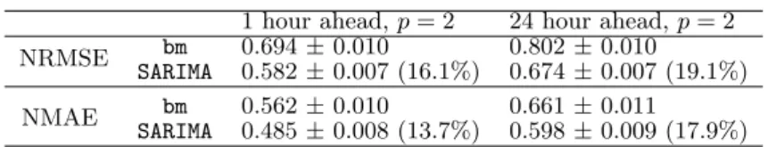
To this end, we apply the stepwise model space exploration algorithm outlined in [22] to each household. Starting from a small set of models, the algorithm iteratively explore the “neighbors” of the best model found so far. The algorithm stops when it cannot find a model better than the current best model. We show the results in Table 3. Although SARIMA provides significantly better forecasts than bench-marks, it does not outperformLR,MLP, orSVR in this case (cf. Table 1 and 2, wherep= 2).
Table 3: Average NRMSE and NMAE (with its 95% con-fidence interval) of Seasonal ARIMA (SARIMA) for 1 hour and 24 hour ahead individual load forecasting. Benchmark (bm) isst−1 for 1 hour ahead forecasting and st−24 for 24
hour ahead forecasting. We use thepth root transformation (st1/p), with p= 2. The numbers in the parentheses show
the improvements compared to the benchmarks.
1 hour ahead,p= 2 24 hour ahead,p= 2
NRMSE bm 0.694±0.010 0.802±0.010
SARIMA 0.582±0.007 (16.1%) 0.674±0.007 (19.1%)
NMAE bm 0.562±0.010 0.661±0.011